


Sage is a powerful tool—but you don't have to take my word for it. This chapter will showcase a few of the things that Sage can do to enhance your work. At this point, don't expect to understand every aspect of the examples presented in this chapter. Everything will be explained in more detail in the later chapters. Look at the things Sage can do, and start to think about how Sage might be useful to you. In this chapter, you will see how Sage can be used for:
Making simple numerical calculations
Performing symbolic calculations
Solving systems of equations and ordinary differential equations
Making plots in two and three dimensions
Analysing experimental data and fitting models
You don't have to install Sage to try it out! In this chapter, we will use the notebook interface to showcase some of the basics of Sage so that you can follow along using a public notebook server. These examples can also be run from an interactive session if you have installed Sage.
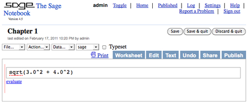
Go to http://www.sagenb.org/ and sign up for a free account. You can also browse worksheets created and shared by others. If you have already installed Sage, launch the notebook interface by following the instructions in Chapter 3. The notebook interface should look like this:

Create a new worksheet by clicking on the link called New Worksheet:

Type in a name when prompted, and click Rename. The new worksheet will look like this:

Enter an expression by clicking in an input cell and typing or pasting in an expression:
Click the evaluate link or press Shift-Enter to evaluate the contents of the cell.
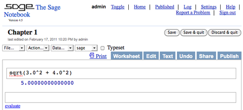
A new input cell will automatically open below the results of the calculation. You can also create a new input cell by clicking in the blank space just above an existing input cell. In Chapter 3, we'll cover the notebook interface in more detail.
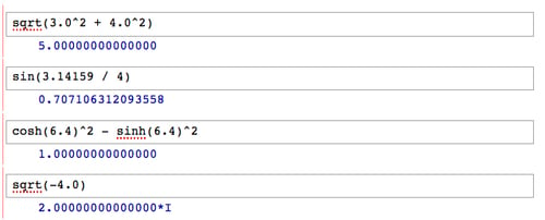
Sage has all the features of a scientific calculator—and more. If you have been trying to perform mathematical calculations with a spreadsheet or the built-in calculator in your operating system, it's time to upgrade. Sage offers all the built-in functions you would expect. Here are a few examples:
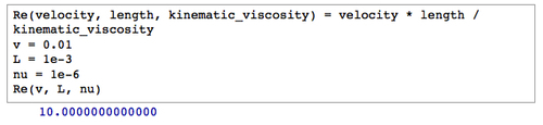
If you have to make a calculation repeatedly, you can define a function and variables to make your life easier. For example, let's say that you need to calculate the Reynolds number, which is used in fluid mechanics:

You can define a function and variables like this:
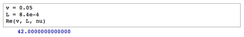
Re(velocity, length, kinematic_viscosity) = velocity * length / kinematic_viscosity

v = 0.01
L = 1e-3
nu = 1e-6
Re(v, L, nu)
When you type the code into an input cell and evaluate the cell, your screen will look like this:
Now, you can change the value of one or more variables and re-run the calculation:
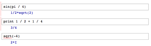
Sage can also perform exact calculations with integers and rational numbers. Using the pre-defined constant
pi will result in exact values from trigonometric operations. Sage will even utilize complex numbers when needed. Here are some examples:
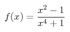
Much of the difficulty of higher mathematics actually lies in the extensive algebraic manipulations that are required to obtain a result. Sage can save you many hours, and many sheets of paper, by automating some tedious tasks in mathematics. We'll start with basic calculus. For example, let's compute the derivative of the following equation:
The following code defines the equation and computes the derivative:
var('x')
f(x) = (x^2 - 1) / (x^4 + 1)
show(f)
show(derivative(f, x))
The results will look like this:
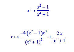
The first line defines a symbolic variable x (Sage automatically assumes that x is always a symbolic variable, but we will define it in each example for clarity). We then defined a function as a quotient of polynomials. Taking the derivative of f(x) would normally require the use of the quotient rule, which can be very tedious to calculate. Sage computes the derivative effortlessly.
Now, we'll move on to integration, which can be one of the most daunting tasks in calculus. Let's compute the following indefinite integral symbolically:
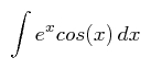
The code to compute the integral is very simple:
f(x) = e^x * cos(x)
f_int(x) = integrate(f, x)
show(f_int)
The result is as follows:
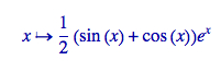
To perform this integration by hand, integration by parts would have to be done twice, which could be quite time consuming. If we want to better understand the function we just defined, we can graph it with the following code:
f(x) = e^x * cos(x)
plot(f, (x, -2, 8))
Sage will produce the following plot:

Sage can also compute definite integrals symbolically:
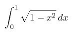
To compute a definite integral, we simply have to tell Sage the limits of integration:
f(x) = sqrt(1 - x^2)
f_integral = integrate(f, (x, 0, 1))
show(f_integral)
The result is:

This would have required the use of a substitution if computed by hand.
There is actually a clever way to evaluate the integral from the previous problem without doing any calculus. If it isn't immediately apparent, plot the function f(x) from 0 to 1 and see if you recognize it. Note that the aspect ratio of the plot may not be square.
The partial fraction decomposition is another technique that Sage can do a lot faster than you. The solution to the following example covers two full pages in a calculus textbook —assuming that you don't make any mistakes in the algebra!
f(x) = (3 * x^4 + 4 * x^3 + 16 * x^2 + 20 * x + 9) / ((x + 2) * (x^2 + 3)^2)
g(x) = f.partial_fraction(x)
show(g)
The result is as follows:
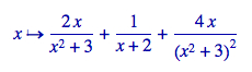
We'll use partial fractions again when we talk about solving ordinary differential equations symbolically.
Linear algebra is one of the most fundamental tasks in numerical computing. Sage has many facilities for performing linear algebra, both numerical and symbolic. One fundamental operation is solving a system of linear equations:
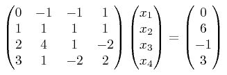
Although this is a tedious problem to solve by hand, it only requires a few lines of code in Sage:
A = Matrix(QQ, [[0, -1, -1, 1], [1, 1, 1, 1], [2, 4, 1, -2],
    [3, 1, -2, 2]])
B = vector([0, 6, -1, 3])
A.solve_right(B)
The answer is as follows:
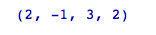
Notice that Sage provided an exact answer with integer values. When we created matrix A, the argument QQ specified that the matrix was to contain rational values. Therefore, the result contains only rational values (which all happen to be integers for this problem). Chapter 5 describes in detail how to do linear algebra with Sage.
Solving ordinary differential equations by hand can be time consuming. Although many differential equations can be handled with standard techniques such as the Laplace transform, other equations require special methods of solution. For example, let's try to solve the following equation:
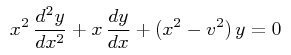
The following code will solve the equation:
var('x, y, v')
y=function('y', x)
assume(v, 'integer')
f = desolve(x^2 * diff(y,x,2) + x*diff(y,x) + (x^2 - v^2) * y == 0,
    y, ivar=x)
show(f)
The answer is defined in terms of Bessel functions:
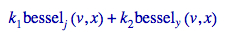
It turns out that the equation we solved is known as Bessel's equation. This example illustrates that Sage knows about special functions, such as Bessel and Legendre functions. It also shows that you can use the assume function to tell Sage to make specific assumptions when solving problems. In Chapter 7, we will explore Sage's powerful symbolic capabilities.
Sage has sophisticated plotting capabilities. By combining the power of the Python programming language with Sage's graphics functions, we can construct detailed illustrations. To demonstrate a few of Sage's advanced plotting features, we will solve a simple system of equations algebraically:
var('x')
f(x) = x^2
g(x) = x^3 - 2 * x^2 + 2

solutions=solve(f == g, x, solution_dict=True)

for s in solutions:
    show(s)
The result is as follows:
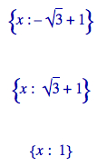
We used the keyword argument solution_dict=True to tell the solve function to return the solutions in the form of a Python list of Python dictionaries. We then used a
for loop to iterate over the list and display the three solution dictionaries. We'll go into more detail about lists and dictionaries in Chapter 4. Let's illustrate our answers with a detailed plot:
p1 = plot(f, (x, -1, 3), color='blue', axes_labels=['x', 'y'])
p2 = plot(g, (x, -1, 3), color='red')

labels = []
lines = []
markers = []
for s in solutions:
    x_value = s[x].n(digits=3)
    y_value = f(x_value).n(digits=3)
    labels.append(text('y=' + str(y_value), (x_value+0.5,
        y_value+0.5), color='black'))
    lines.append(line([(x_value, 0), (x_value, y_value)],
        color='black', linestyle='--'))
    markers.append(point((x_value,y_value), color='black', size=30))

show(p1+p2+sum(labels) + sum(lines) + sum(markers))
The plot looks like this:
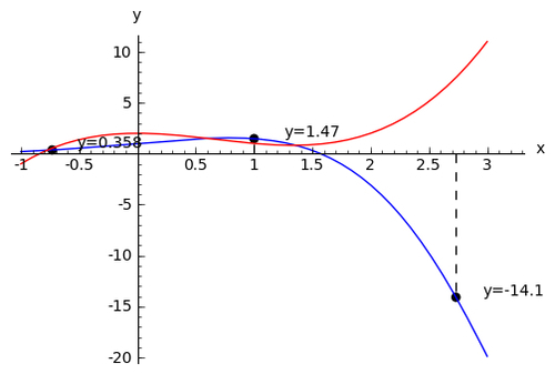
We created a plot of each function in a different colour, and labelled the axes. We then used another for loop to iterate through the list of solutions and annotate each one. Plotting will be covered in detail in Chapter 6.
Sage does not restrict you to making plots in two dimensions. To demonstrate the 3D capabilities of Sage, we will create a parametric plot of a mathematical surface known as the "figure 8" immersion of the Klein bottle. You will need to have Java enabled in your web browser to see the 3D plot.
var('u,v')
r = 2.0
f_x = (r + cos(u / 2) * sin(v) - sin(u / 2)
    * sin(2 * v)) * cos(u)
f_y = (r + cos(u / 2) * sin(v) - sin(u / 2)
    * sin(2 * v)) * sin(u)
f_z = sin(u / 2) * sin(v) + cos(u / 2) * sin(2 * v)
parametric_plot3d([f_x, f_y, f_z], (u, 0, 2 * pi),
    (v, 0, 2 * pi), color="red")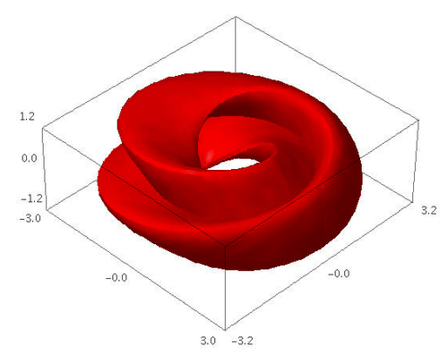
In the Sage notebook interface, the 3D plot is fully interactive. Clicking and dragging with the mouse over the image changes the viewpoint. The scroll wheel zooms in and out, and right-clicking on the image brings up a menu with further options.
Sage can be used in conjunction with the LaTeX typesetting system to create publication-quality typeset mathematical expressions. In fact, all of the mathematical expressions in this chapter were typeset using Sage and exported as graphics. Chapter 10 explains how to use LaTeX and Sage together.
One of the most common tasks for an engineer or scientist is analysing data from an experiment. Sage provides a set of tools for loading, exploring, and plotting data. The following series of examples shows how a scientist might analyse data from a population of bacteria that are growing in a fermentation tank. Someone has measured the optical density (abbreviated OD) of the liquid in the tank over time as the bacteria are multiplying. We want to analyse the data to see how the size of the population of bacteria varies over time. Please note that the examples in this section must be run in order, since the later examples depend upon results from the earlier ones.
The optical density is correlated to the concentration of bacteria in the liquid. To quantify this correlation, someone has measured the optical density of a number of calibration standards of known concentration. In this example, we will fit a "standard curve" to the calibration data that we can use to determine the concentration of bacteria from optical density readings:
import numpy
var('OD, slope, intercept')

def standard_curve(OD, slope, intercept):
    """Apply a linear standard curve to optical density data"""
    return OD * slope + intercept

# Enter data to define standard curve
CFU = numpy.array([2.60E+08, 3.14E+08, 3.70E+08, 4.62E+08,
    8.56E+08, 1.39E+09, 1.84E+09])
optical_density = numpy.array([0.083, 0.125, 0.213, 0.234,
    0.604, 1.092, 1.141])
OD_vs_CFU = zip(optical_density, CFU)

# Fit linear standard
std_params = find_fit(OD_vs_CFU, standard_curve,
    parameters=[slope, intercept],
    variables=[OD], initial_guess=[1e9, 3e8],
    solution_dict = True)

for param, value in std_params.iteritems():
    print(str(param) + ' = %e' % value)

# Plot
data_plot = scatter_plot(OD_vs_CFU, markersize=20,
    facecolor='red', axes_labels=['OD at 600nm', 'CFU/ml'])

fit_plot = plot(standard_curve(OD, std_params[slope],
    std_params[intercept]), (OD, 0, 1.2))

show(data_plot+fit_plot)
The results are as follows:
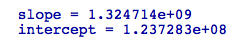
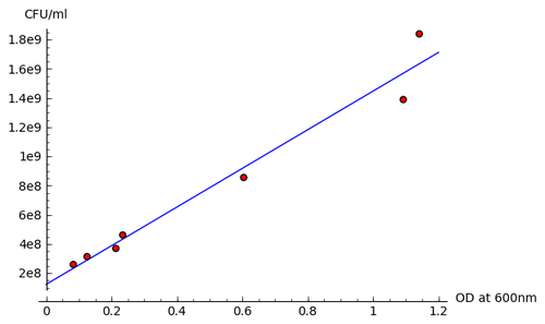
We introduced some new concepts in this example. On the first line, the statement import numpy allows us to access functions and classes from a module called NumPy. NumPy is based upon a fast, efficient array class, which we will use to store our data. We created a NumPy array and hard-coded the data values for OD, and created another array to store values of concentration (in practice, we would read these values from a file) We then defined a Python function called
standard_curve, which we will use to convert optical density values to concentrations. We used the
find_fit function to fit the slope and intercept parameters to the experimental data points. Finally, we plotted the data points with the scatter_plot function and the plotted the fitted line with the plot function. Note that we had to use a function called
zip to combine the two NumPy arrays into a single list of points before we could plot them with scatter_plot. We'll learn all about Python functions in Chapter 4, and Chapter 8 will explain more about fitting routines and other numerical methods in Sage.
Now that we've defined the relationship between the optical density and the concentration of bacteria, let's look at a series of data points taken over the span of an hour. We will convert from optical density to concentration units, and plot the data.
sample_times = numpy.array([0, 20, 40, 60, 80, 100, 120,
    140, 160, 180, 200, 220, 240, 280, 360, 380, 400, 420,
    440, 460, 500, 520, 540, 560, 580, 600, 620, 640, 660,
    680, 700, 720, 760, 1240, 1440, 1460, 1500, 1560])

OD_readings = numpy.array([0.083, 0.087, 0.116, 0.119, 0.122,
    0.123, 0.125, 0.131, 0.138, 0.142, 0.158, 0.177, 0.213,
    0.234, 0.424, 0.604, 0.674, 0.726, 0.758, 0.828, 0.919,
    0.996, 1.024, 1.066, 1.092, 1.107, 1.113, 1.116, 1.12,
    1.129, 1.132, 1.135, 1.141, 1.109, 1.004, 0.984, 0.972, 0.952])

concentrations = standard_curve(OD_readings, std_params[slope],
     std_params[intercept])
exp_data = zip(sample_times, concentrations)

data_plot = scatter_plot(exp_data, markersize=20, facecolor='red',
    axes_labels=['time (sec)', 'CFU/ml'])
show(data_plot)
The scatter plot looks like this:
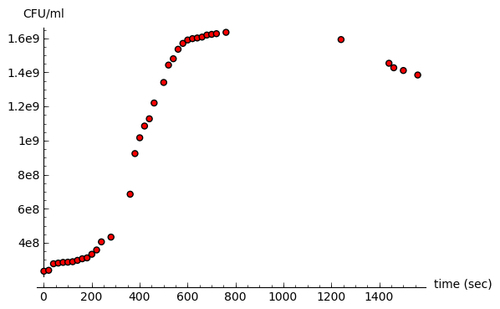
We defined one NumPy array of sample times, and another NumPy array of optical density values. As in the previous example, these values could easily be read from a file. We used the standard_curve function and the fitted parameter values from the previous example to convert the optical density to concentration. We then plotted the data points using the scatter_plot function.
Now, let's fit a growth model to this data. The model we will use is based on the Gompertz function, and it has four parameters:
var('t, max_rate, lag_time, y_max, y0')
def gompertz(t, max_rate, lag_time, y_max, y0):
"""Define a growth model based upon the Gompertz growth curve"""
return y0 + (y_max - y0) * numpy.exp(-numpy.exp(1.0 +
max_rate * numpy.exp(1) * (lag_time - t) / (y_max - y0)))
# Estimated parameter values for initial guess
max_rate_est = (1.4e9 - 5e8)/200.0
lag_time_est = 100
y_max_est = 1.7e9
y0_est = 2e8
gompertz_params = find_fit(exp_data, gompertz,
parameters=[max_rate, lag_time, y_max, y0],
variables=[t],
initial_guess=[max_rate_est, lag_time_est, y_max_est, y0_est],
solution_dict = True)
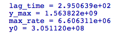
for param,value in gompertz_params.iteritems():
print(str(param) + ' = %e' % value)The fitted parameter values are displayed:
Finally, let's plot the fitted model and the experimental data points on the same axes:
gompertz_model_plot = plot(gompertz(t, gompertz_params[max_rate],
    gompertz_params[lag_time], gompertz_params[y_max],
    gompertz_params[y0]), (t, 0, sample_times.max()))

show(gompertz_model_plot + data_plot)
The plot looks like this:
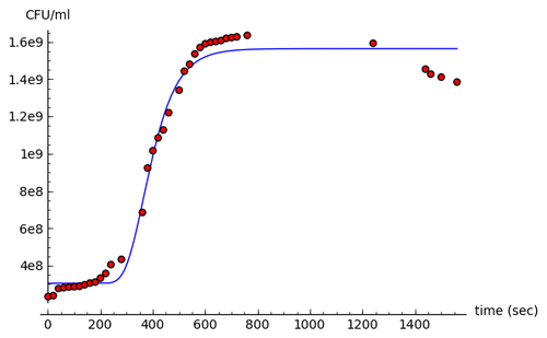
We defined another Python function called gompertz
to model the growth of bacteria in the presence of limited resources. Based on the data plot from the previous example, we estimated values for the parameters of the model to use an initial guess for the fitting routine. We used the find_fit function again to fit the model to the experimental data, and displayed the fitted values. Finally, we plotted the fitted model and the experimental data on the same axes.
This chapter has given you a quick, high-level overview of some of the many things that Sage can do for you. Don't worry if you feel a little lost, or if you had trouble trying to modify the examples. Everything you need to know will be covered in detail in later chapters.
Specifically, we looked at:
Using Sage as a sophisticated scientific and graphing calculator
Speeding up tedious tasks in symbolic mathematics
Solving a system of linear equations, a system of algebraic equations, and an ordinary differential equation
Making publication-quality plots in two and three dimensions
Using Sage for data analysis and model fitting in a practical setting
Hopefully, you are convinced that Sage will be the right tool to assist you in your work, and you are ready to install Sage on your computer. In the next chapter, you will learn how to install Sage on various platforms.

