This chapter intends to provide context and background to set the base with which we can manipulate the datasets to be used for data modeling. This section tries to act as a refresher that should help you understand and pick up modeling topics faster in upcoming chapters.
We start the chapter with Structured Query Language (SQL)—how we can use it for controlling and manipulating the SAP HANA database objects and data. Then we move on to create SQLscript and learn how to use it effectively. We will also discuss creation and call of procedure step by step in this chapter, which is a good tool for the upcoming topics. We will end the chapter with a detailed discussion on JOINS and how it can be used for connecting tables in SAP HANA.
After completing this chapter you will be able to:
Understand and use SAP HANA SQL statements
Create SQLscript and use it
Create and call a procedure
Connect tables using SAP HANA specific JOINS
As stated, you will not learn SQL as a whole new concept, but will just revise the traditional SQL concepts at a glance and focus on a few new topics that are of importance from SAP HANA perspective. Our key focus here will be on the SAP HANA SQL script, creating procedures, and learning to create SAP HANA specific JOINS.
SQL is used to retrieve, store, and manipulate data in the database. SQL can be studied under three subheads:

These subheads are explained as follows:
DDL: These statement that are used to define the data:
create,alter,droptablesDML: These statements are used to manipulate the data,
select,deselect,insert, andupdateDCL: These statements that are used to control the
table,grant, and revoke
The followings are the elements of SQL:
Identifiers: These are used to represent names in SQL statements including table/view name, column name, username, role name and so on. There are two types of Identifiers: ordinary and delimited.
Data types: These define the characteristics of the data and its value. Data types in SQL are as follows:
Categories
Data type
Numeric
float,real,integer,decimal,double,tinyint,small int, andsmall decimalLarge
blob,clob,nclob, andtextBinary
varbinaryCharacter string
varchar,nvarchar,alphanum, andshorttext.Date
time,date,secondtime, andtimestampExpressions: These are clause evaluated to return values. We have different types of expressions in SQL. For example,
if…then…..else(case expression) or nested queries (Select (Select ……)).Functions: These are used in expressions for retrieving information from the database. We have a number of functions and data type conversion functions. The number functions take numeric values or alphanumeric/strings with numeric character values and return numeric values, whereas, data type conversion functions are used to convert arguments from one data type to another. For example,
to_alphanum,concat,current_date, and so on.Operators: These are used for value comparison, assigning values, or can also be used for calculation. We have different types of operators like Unary, Binary, arithmetic, and string operators to name a few. For example,
+,=,subtraction, andor.Predicates: A predicate is specified by combining one or more expressions or logical operators and returning one of the following logical or truth values: true, false, or unknown. Examples are null, in, and like.
In the upcoming chapters, we will learn how to work with SAP HANA studio and open SQL editor, so as to complete the concepts. I will show you how we work with the preceding SQL concepts. For our examples and exercises, we will use the following tables. We will create more tables in further chapters as we progress.
The following table shows you the sales_facts:
|
|
|
|
|
|
|
|
|
|
|
|
|
|
|
|
|
|
|
|
The following table shows you the CUSTOMERS data:
|
|
|
|
|
|
|
|
|
|
|
|
|
|
|
|
The following is a REGION table:
|
|
|
|
|
|
|
|
|
|
|
|
|
|
|
|
The following table shows you details of the PRODUCT table:
|
|
|
|
|
|
|
|
|
Let's see how we can create the preceding tables in SAP HANA:
In SAP HANA studio, right-clicking on your schema (here, HANA_DEMO) will display Open SQL Console; click on it.

We will cover some of the following SQL queries to create the tables:
Create a schema first, if it hasn't already been created for you—
HANA_DEMO; you can choose any name.A database schema is the skeleton structure that represents the logical view of the entire database (objects such as tables, views, and stored procedures). It defines how the data is organized and how the relations among them are associated. It formulates all the constraints that are to be applied on the data, whereas
Tableis one of the objects contained in schema. It is a set of data elements (values) that is organized using a model of vertical columns (which are identified by their name) and horizontal rows:CREATE SCHEMA "HANA_DEMO"; GRANT SELECT ON SCHEMA HANA_DEMO TO _SYS_REPO WITH GRANT OPTION; if you do not run Grant , later when you will activate your views it will give you erros.
The following command creates the
SALES_FACTStable:CREATE COLUMN TABLE "HANA_DEMO"."SALES_FACTS"( "PRODUCT_KEY" INTEGER NOT NULL, "REGION_KEY" INTEGER NOT NULL, "AMOUNT_SOLD" DECIMAL NOT NULL, "QUANTITY_SOLD" INTEGER NOT NULL, PRIMARY KEY ("PRODUCT_KEY","REGION_KEY") );
The following command creates the
CUSTOMERtable:CREATE COLUMN TABLE "HANA_DEMO"."CUSTOMER"( "CUSTOMER_KEY" VARCHAR(8) NOT NULL, "CUST_LAST_NAME" VARCHAR(100) NULL, "CUST_FIRST_NAME" VARCHAR(30) NULL, PRIMARY KEY ("CUSTOMER_KEY ") );
The following command creates the
PRODUCTStable:CREATE COLUMN TABLE "HANA_DEMO"."PRODUCTS" ( "PRODUCT_KEY" INTEGER NOT NULL, "PRODUCT_NAME" VARCHAR(50) NULL, PRIMARY KEY ("PRODUCT_KEY") );
The following command creates the
REGIONtable:CREATE COLUMN TABLE "HANA_DEMO"."REGION"( "REGION_ID" INTEGER NOT NULL, "REGION_NAME" VARCHAR(100) NULL, "SUB_AREA" VARCHAR(30) NULL, PRIMARY KEY ("REGION_ID") );
The following are sample
insertqueries:insert into "<YOUR SCHEMA>"."TABLE NAME" values(columns1,Columns2,..,); insert into "HANA_DEMO"."SALES_FACTS" values(01,100,50000,500); insert into "HANA_DEMO"."PRODUCTS" values(01,'GasKit'); insert into "HANA_DEMO"."REGION" values(01,'Europe','Germany');
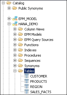
After executing the scripts, you should have three tables created. If there are no tables, try right-clicking on your schema and then refresh it.
In the following screenshot, you can see the tables we just created under the HANA_DEMO schema:
In SQL, the editor of our schema needs to execute the following command line:
GRANT SELECT ON SCHEMA <YOUR SCHEMA> TO _SYS_REPO WITH GRANT OPTION;
GRANT SELECT ON SCHEMA HANA_DEMO TO _SYS_REPO WITH GRANT OPTION
If we miss this step, an error will occur when you activate your views later.
In the following section, we will learn about the SAP HANA SQLscript and see the additional capabilities it brings along with it.
SQLscript is a collection of extensions in Structured Query Language (SQL). The main motivation for SQLscript is to push data intensive application logic into the database, which was not being done in the classical approach where the application logic is mostly executed in an application layer.
We have the following extensions for SQLscript:
Let's do a comparative study between an SQLscript in SAP HANA and classical SQL queries to find out what the point of differences are, as shown in the following table:
|
SQLscript in SAP HANA |
Classical SQL |
|---|---|
|
Multiple result sets can be returned |
Query returns only single result set |
|
More database intensive, codes are executed at DB layer, gives better performance |
Limited executions at DB layer resulting in multiple access to and from database, relatively slow performance |
|
Control logics such as if/else and business logics like currency conversion can be easily expressed |
SQL queries do not have such features |
|
Gives more flexibility to developer to use imperative and declarative logics together |
No such flexibility with SQL queries |
|
Supports local variables for intermediate result sets with implicit types |
Globally visible views need to be defined even for intermediate result sets or steps |
|
Parameterization of views is possible |
Parameterization of views is not possible |
The following figure shows you a graphical comparison of the classical approach and the SAP HANA approach:

Procedures are reusable processing blocks that are implemented using the SQLscript, which describes a sequence of operations on data passed as input and database tables. It can be created as read-only (without side-effects) or read-write (with side-effects).
Procedures can have multiple input parameters and output parameters (can be scalar or table types).
There are three different ways to create a procedure in HANA:
Using the SQL editor (in SAP HANA Studio)
Using the Modeler wizard in the modeler perspective (in SAP HANA Studio)
Using the SAP HANA XS project in the SAP HANA Development perspective (in SAP HANA Studio), which isn't discussed in this chapter
The following syntax is used to create procedure via the SQL editor:
CREATE PROCEDURE {schema.}name
            {({IN|OUT|INOUT}
                        param_name data_type {,...})}
            {LANGUAGE <LANG>} {SQL SECURITY <MODE>}
            {READS SQL DATA {WITH RESULT VIEW <view_name>}} AS
BEGIN
...
END
Tip
Downloading the example code
You can download the example code files from your account at http://www.packtpub.com for all the Packt Publishing books you have purchased. If you purchased this book elsewhere, you can visit http://www.packtpub.com/support and register to have the files e-mailed directly to you.
The parameters are for:
Let's create a procedure where we will pass discount as the input parameter and get the sales report as the output parameter. We use the same tables that we created previously:
CREATE PROCEDURE HANA_DEMO."PROC_EU_SALES_REPORT"(
            IN DISCOUNT INTEGER,
            OUT OUTPUT_TABLE HANA_DEMO."EU_SALES" )
LANGUAGE SQLSCRIPT SQL SECURITY INVOKER AS
/*********BEGIN PROCEDURE SCRIPT ************/
BEGIN
Pvar1 = SELECT T1.REGION_NAME, T1.SUB_AREA, T2.PRODUCT_KEY, T2.AMOUNT_SOLD
            FROM HANA_DEMO.REGION AS T1
            INNER JOIN
            HANA_DEMO.SALES_FACT AS T2
            ON T1.REGION_KEY = T2.REGION_KEY;

Pvar2 = SELECT T1.REGION_NAME, T1.SUB_AREA, T1.PRODUCT_KEY, T1.AMOUNT_SOLD, T2.PRODUCT_NAME
            FROM :Pvar1 AS T1
            INNER JOIN
            HANA_DEMO.PRODUCT AS T2
            ON T1.PRODUCT_KEY = T2.PRODUCT_KEY;

OUTPUT_TABLE = SELECT SUM(AMOUNT_SOLD) AS AMOUNT_SOLD, SUM(AMOUNT_SOLD - (AMOUNT_SOLD * :DISCOUNT/ 100)) AS NET_AMOUNT,
            PRODUCT_NAME, REGION_NAME, SUB_AREA
            FROM :Pvar2
            GROUP BY PRODUCT_NAME, REGION_NAME, SUB_AREA;
END;
We can call the previously created procedure with the following CALL statement:
CALL HANA_DEMO."PROC_SALES_REPORT" (8, null);
You can see the created procedure below our schema under the Procedure... folder.

Choose the package in which you want to create the procedure and right-click on it.
A new screen will pop up; fill in the details and click on Confirm:

The SQL console opens with default syntax; we need to put our logic in between BEGIN and END.
The following is a sample logic with which I am creating the Procedure:

On the left-hand side of the screen, you can see the output pane:

Click on it and select New…:

Define the columns which we used in the preceding procedure:

Similarly, perform the same steps for input parameters as well:

Now the procedure is ready to be called via the CALL statement.
Once we build our concept about different views, then one question that will definitely come to our mind is, should we use calculation views (not yet discussed) or procedures. We will discuss this once we have discussed the calculation view in Chapter 5, Creating SAP HANA Artifacts – Analytical Privileges and Calculation Views.
To address some specific business cases and have improved execution, SAP HANA introduces some additional JOINS on top of existing SQL JOINS. These SAP HANA specific JOINS are as follows:
Referential JOIN
Text JOIN
Temporal JOIN
Star JOIN
Spatial JOIN
Let's see the scenarios when we should consider using these SAP HANA specific JOINS :
Unions are used to combine the result set of two or more SELECT statements. It's always tempting to JOIN two analytic views when measures from more than one table are required. This should, however, be avoided for performance reasons. It is more beneficial to use a Union in a calculation view. Technically, a Union is not a JOIN type.
Points to remember:
Union is not supported in the attribute or analytical view but can only be used in calculation views.
Union with constant values are supported within graphical calculation views and the Union operator can accept 1..N input sources.
Script-based calculation views can only accept two input sources at a given time.
Do not JOIN analytical views (to be discussed later), as you might have performance issues. Instead, use Union with constant values when working with multiple fact tables.
With this chapter, we set the base for the book. It was expected that you already knew these topics and the chapter refreshed them for you. We started with the basics of SQL and how to use SAP HANA SQL statements. We progressed to create SQLscript and procedure. Towards the closure of the chapter, you learned about additional JOINS that SAP HANA has to improve business scenarios, and we closed the chapter with a discussion on Union and JOINS.
In the next chapter, we will cover the approach to SAP HANA data modeling and the dos and don'ts while creating data models. You will also learn which kind of view should be created for different types of information.