


This chapter covers the following topics:
Creating R functions
Matching arguments
Understanding environments
Working with lexical scope
Understanding closure
Performing lazy evaluation
Creating infix operators
Using the replacement function
Handling errors in a function
The debugging function
R is the mainstream programming language of choice for data scientists. According to polls conducted by KDnuggets, a leading data analysis website, R ranked as the most popular language for analytics, data mining, and data science in the three most recent surveys (2012 to 2014). For many data scientists, R is more than just a programming language because the software also provides an interactive environment that can perform all types of data analysis.
R has many advantages in data manipulation and analysis, and the three most well-known are as follows:
Open Source and free: Using SAS or SPSS requires the purchase of a usage license. One can use R for free, allowing users to easily learn how to implement statistical algorithms from the source code of each function.
Powerful data analysis functions: R is famous in the data science community. Many biologists, statisticians, and programmers have wrapped their models into R packages before distributing these packages worldwide through CRAN (Comprehensive R Archive Network). This allows any user to start their analysis project by downloading and installing an R package from CRAN.
Easy to use: As R is a self-explanatory, high-level language, programming in R is fairly easy. R users only need to know how to use the R functions and how each parameter works through its powerful documentation. We can easily conduct high-level data analysis without having knowledge of the complex underlying mathematics.
R users will most likely agree that these advantages make complicated data analysis easier and more approachable. Notably, R also allows us to take the role of just a basic user or a developer. For an R user, we only need to know how a function works without requiring detailed knowledge of how it is implemented. Similarly to SPSS, we can perform various types of data analysis through R's interactive shell. On the other hand, as an R developer, we can write their function to create a new model, or they can even wrap implemented functions into a package.
Instead of explaining how to write an R program from scratch, the aim of this book is to cover how to become a developer in R. The main purpose of this chapter is to show users how to define their function to accelerate the analysis procedure. Starting with creating a function, this chapter covers the environment of R, and it explains how to create matching arguments. There is also content on how to perform functional programming in R, how to create advanced functions, such as infix operator and replacement, and how to handle errors and debug functions.
The R language is a collection of functions; a user can apply built-in functions from various packages to their project, or they can define a function for a particular purpose. In this recipe, we will show you how to create an R function.
If you are new to the R language, you can find a detailed introduction, language history, and functionality on the official R site (http://www.r-project.org/). When you are ready to download and install R, please connect to the comprehensive R archive network (http://cran.r-project.org/).
Perform the following steps in order to create your first R function:
Type the following code on your R console to create your first function:
>addnum<- function(x, y){
+ s <- x+y
+ return(s)
+ }
Execute the
addnumuser-defined function with the following command:>addnum (3,7) [1] 10
Or, you can define your function without a
returnstatement:>addnum2<- function(x, y){ + x+y + }
Execute the
addnum2user-defined function with the following command:>addnum2(3,7) [1] 10
You can view the definition of a function by typing its function name:
>addnum2
function(x, y){
x+y
}
Finally, you can use body and formals to examine the
bodyandformalarguments of a function:>body(addnum2) { x + y } >formals(addnum2) $x $y >args(addnum2) function (x, y) NULL
R functions are a block of organized and reusable statements, which makes programming less repetitive by allowing you to reuse code. Additionally, by modularizing statements within a function, your R code will become more readable and maintainable.
By following these steps, you can now create two addnum and addnum2 R functions, and you can successfully add two input arguments with either function. In R, the function usually takes the following form:
FunctionName<- function (arg1, arg2) {
body
return(expression)
}
FunctionName is the name of the function, and arg1 and arg2 are arguments. Inside the curly braces, we can see the function body, where a body is a collection of a valid statement, expression, or assignment. At the bottom of the function, we can find the return statement, which passes expression back to the caller and exits the function.
The addnum function is in standard function syntax, which contains both body and return statement. However, you do not necessarily need to put a return statement at the end of the function. Similar to the addnum2 function, the function itself will return the last expression back to the caller.
If you want to view the composition of the function, simply type the function name on the interactive shell. You can also examine the body and formal arguments of the function further using the body and formal functions. Alternatively, you can use the args function to obtain the argument list of the function.
In R functions, the arguments are the input variables supplied when you invoke the function. We can pass the argument, named argument, argument with default variable, or unspecific numbers of argument into functions. In this recipe, we will demonstrate how to pass different kinds of arguments to our defined function.
Perform the following steps to create a function with different types of argument lists:
Type the following code to your R console to create a function with a default value:
>defaultarg<- function(x, y = 5){
+ y <- y * 2
+ s <- x+y
+ return(s)
+ }
Then, execute the
defaultarguser-defined function by passing3as the input argument:>defaultarg(3) [1] 13
Alternatively, you can pass different types of input argument to the function:
>defaultarg(1:3)
[1] 11 12 13
You can also pass two arguments into the function:
>defaultarg(3,6)
[1] 15
Or, you can pass a named argument list into the function:
>defaultarg(y = 6, x = 3)
[1] 15
Moving on, you can use if-else-condition together with the function of the named argument:
>funcarg<- function(x, y, type= "sum"){
+ if (type == "sum"){
+ sum(x,y)
+ }else if (type == "mean"){
+ mean(x,y)
+ }else{
+ x * y
+ }
+ }
>funcarg(3,5)
[1] 8
>funcarg(3,5, type = 'mean')
[1] 3
>funcarg(3,5, type = 'unknown')
[1] 15
Additionally, one can pass an unspecified number of parameters to the function:
>unspecarg<- function(x, y, ...){
+ x <- x + 2
+ y <- y * 2
+ sum(x,y, ...)
+ }
>unspecarg(3,5)
[1] 15
>unspecarg(3,5,7,9,11)
[1] 42
R provides a flexible argument binding mechanism when creating functions. In this recipe, we first create a function called defaultag with two formal arguments: x and y. Here, the y argument has a default value, defined as 5. Then, when we make a function call by passing 3 to defaultarg, it passes 3 to x and 5 to y in the function and returns 13. Besides passing a scalar as the function input, we can pass a vector (or any other data type) to the function. In this example, if we pass a 1:3 vector to defaultarg, it returns a vector.
Moving on, we can see how arguments bind to the function. When calling a function by passing an argument without a parameter name, the function binds the passing value by position. Take step 4 as an example; the first 3 argument matches to x, and 6 matches to y, and it returns 15. On the other hand, you can pass arguments by name. In step 5, we can pass named arguments to the function in any order. Thus, if we pass y=6 and x=3 to defaultarg, the function returns 15.
Furthermore, we can use an argument as a control statement. In step 6, we specify three formal arguments: x, y, and type, in which the type argument has the default value defined as sum. Next, we can specify the value for the type argument as a condition in the if-else control flow. That is, when we pass sum to type, it returns the summation of x and y. When we pass mean to type, it returns the average of x and y. When we pass any value other than sum and mean to the type argument, it returns the product of x and y.
Lastly, we can pass an unspecified number of arguments to the function using the ... notation. In the final step of this example, if we pass only 3 and 5 to the function, the function first passes 3 to x and 5 to y. Then, the function adds 2 to x, multiplies y by 2, and sums the value of both x and y. However, if we pass more than two arguments to the function, the function will also sum the additional parameters.
In addition to giving a full argument name, we can abbreviate the argument name when making a function call:
>funcarg(3,5, t = 'unknown')
[1] 15
Here, though we do not specify the argument's name, type, correctly, the function passes a value of unknown to the argument type, and returns 15 as the output.
Besides the function name, body, and formal arguments, the environment is another basic component of a function. In a nutshell, the environment is where R manages and stores different types of variables. Besides the global environment, each function activates its environment whenever a new function is created. In this recipe, we will show you how the environment of each function works.
Ensure that you completed the previous recipes by installing R on your operating system.
Perform the following steps to work with the environment:
First, you can examine the current environment with the
environmentfunction:>environment() <environment: R_GlobalEnv>
You can also browse the global environment with
.GlobalEnvandglobalenv:> .GlobalEnv <environment: R_GlobalEnv> >globalenv() <environment: R_GlobalEnv>
You can compare the environment with the
identicalfunction:>identical(globalenv(), environment()) [1] TRUE
Furthermore, you can create a new environment as follows:
>myenv<- new.env()
>myenv
<environment: 0x0000000017e3bb78>
Next, you can find the variables of different environments:
>myenv$x<- 3
>ls(myenv)
[1] "x"
>ls()
[1] "myenv"
>x
Error: object 'x' not found
At this point, you can create an
addnumfunction and useenvironmentto get the environment of the function:>addnum<- function(x, y){ + x+y + } >environment(addnum) <environment: R_GlobalEnv>
You can also determine that the environment of a function belongs to the package:
>environment(lm)
<environment: namespace:stats>
Moving on, you can print the environment within a function:
>addnum2<- function(x, y){
+ print(environment())
+ x+y
+ }
>addnum2(2,3)
<environment: 0x0000000018468710>
[1] 5
Furthermore, you can compare the environment inside and outside a function:
>addnum3<- function(x, y){
+ func1<- function(x){
+ print(environment())
+ }
+ func1(x)
+ print(environment())
+ x + y
+ }
>addnum3(2,5)
<environment: 0x000000001899beb0>
<environment: 0x000000001899cc50>
[1] 7
We can regard an R environment as a place to store and manage variables. That is, whenever we create an object or a function in R, we add an entry to the environment. By default, the top-level environment is the R_GlobalEnv global environment, and we can determine the current environment using the environment function. Then, we can use either .GlobalEnv or globalenv to print the global environment, and we can compare the environment with the identical function.
Besides the global environment, we can actually create our environment and assign variables into the new environment. In the example, we created the myenv environment and then assigned x <- 3 to myenv by placing a dollar sign after the environment name. This allows us to use the ls function to list all variables in myenv and global environment. At this point, we find x in myenv, but we can only find myenv in the global environment.
Moving on, we can determine the environment of a function. By creating a function called addnum, we can use environment to get its environment. As we created the function under global environment, the function obviously belongs to the global environment. On the other hand, when we get the environment of the lm function, we get the package name instead. That means that the lm function is in the namespace of the stat package.
Furthermore, we can print out the current environment inside a function. By invoking the addnum2 function, we can determine that the environment function outputs a different environment name from the global environment. That is, when we create a function, we also create a new environment for the global environment and link a pointer to its parent environment. To further examine this characteristic, we create another addnum3 function with a func1 nested function inside. At this point, we can print out the environment inside func1 and addnum3, and it is possible that they have completely different environments.
To get the parent environment, we can use the parent.env function. In the following example, we can see that the parent environment of parentenv is R_GlobalEnv:
>parentenv<- function(){
+ e <- environment()
+ print(e)
+ print(parent.env(e))
+ }
>parentenv()
<environment: 0x0000000019456ed0>
<environment: R_GlobalEnv>
Lexical scoping, also known as static binding, determines how a value binds to a free variable in a function. This is a key feature that originated from the scheme functional programming language, and it makes R different from S. In the following recipe, we will show you how lexical scoping works in R.
Perform the following steps to understand how the scoping rule works:
First, we create an
xvariable, and we then create atmpfuncfunction withx+3as the return:>x<- 5 >tmpfunc<- function(){ + x + 3 + } >tmpfunc() [1] 8
We then create a function named
parentfuncwith achildfuncnested function and see what returns when we call theparentfuncfunction:>x<- 5 >parentfunc<- function(){ + x<- 3 + childfunc<- function(){ + x + } + childfunc() + } >parentfunc() [1] 3
Next, we create an
xstring, and then we create alocalassignfunction to modifyxwithin the function:> x <- 'string' >localassign<- function(x){ + x <- 5 + x + } >localassign(x) [1] 5 >x [1] "string"
We can also create another
globalassignfunction but reassign thexvariable to5using the<<-notation:> x <- 'string' >gobalassign<- function(x){ + x <<- 5 + x + } >gobalassign(x) [1] 5 >x [1] 5
There are two different types of variable binding methods: one is lexical binding, and the other is dynamic binding. Lexical binding is also called static binding in which every binding scope manages variable names and values in the lexical environment. That is, if a variable is lexically bound, it will search the binding of the nearest lexical environment. In contrast to this, dynamic binding keeps all variables and values in the global state. That is, if a variable is dynamically bound, it will bind to the most recently created variable.
To demonstrate how lexical binding works, we first create an x variable and assign 5 to x in the global environment. Then, we can create a function named tmpfunc. The function outputs x + 3 as the return value. Even though we do not assign any value to x within the tmpfunc function, x can still find the value of x as 5 in the global environment.
Next, we create another function named parentfunc. In this function, we assign x to 3 and create a childfunc nested function (a function defined within a function). At the bottom of the parentfunc body, we invoke childfunc as the function return. Here, we find that the function uses the x defined in parentfunc instead of the one defined outside parentfunc. This is because R searches the global environment for a matched symbol name, and then subsequently searches the namespace of packages on the search list.
Moving on, let's take a look at what will return if we create an x variable as a string in the global state and assign an x local variable to 5 within the function. When we invoke the localassign function, we discover that the function returns 5 instead of the string value. On the other hand, if we print out the value of x, we still see string in return. While the local variable and global variable have the same name, the assignment of the function does not alter the value of x in global state. If you need to revise the value of x in the global state, you can use the <<- notation instead.
Functions are the first-class citizens of R. In other words, you can pass a function as the input to an other function. In previous recipes, we illustrated how to create a named function. However, we can also create a function without a name, known as closure (that is, an anonymous function). In this recipe, we will show you how to use closure in a standard function.
Ensure that you completed the previous recipes by installing R on your operating system.
Perform the following steps to create a closure in function:
First, let's review how a named function works:
>addnum<- function(a,b){
+ a + b
+ }
>addnum(2,3)
[1] 5
Now, let's perform the same task to sum up two variables with closure:
> (function(a,b){
+ a + b
+ })(2,3)
[1] 5
We can also invoke a closure function within another function:
>maxval<- function(a,b){
+ (function(a,b){
+ return(max(a,b))
+ }
+ )(a, b)
+ }
>maxval(c(1,10,5),c(2,11))
[1] 11
In a similar manner to the apply family function, you can use the vectorization calculation:
> x <- c(1,10,100)
> y <- c(2,4,6)
> z <- c(30,60,90)
> a <- list(x,y,z)
>lapply(a, function(e){e[1] * 10})
[[1]]
[1] 10
[[2]]
[1] 20
[[3]]
[1] 300
Finally, we can add functions into a list and apply the function to a given vector:
> x <- c(1,10,100)
>func<- list(min1 = function(e){min(e)},
 max1 = function(e){max(e)} )
>func$min1(x)
[1] 1
>lapply(func, function(f){f(x)})
$min1
[1] 1
$max1
[1] 100
In R, you do not have to create a function with the actual name. Instead, you can use closure to integrate methods within objects. Thus, you can create a smaller and simpler function within another object to accomplish complicated tasks.
In our first example, we illustrated how a normally-named function is created. We can simply invoke the function by passing values into the function. On the other hand, we demonstrate how closure works in our second example. In this case, we do not need to assign a name to the function, but we can still pass the value to the anonymous function and obtain the return value.
Next, we demonstrate how to add a closure within a maxval named function. This function simply returns the maximum value of two passed parameters. However, it is possible to use closure within any other function. Moreover, we can use closure as an argument in higher order functions, such as lapply and sapply. Here, we can input an anonymous function as a function argument to return the multiplication of 10 and the first value of any vector within a given list.
Furthermore, we can specify a single function, or we can store functions in a list. Therefore, when we want to apply multiple functions to a given vector, we can pass the function calls as an argument list to the lapply function.
Besides using closure within a lapply function, we can also pass a closure to other functions of the apply function family. Here, we demonstrate how we can pass the same closure to the sapply function:
> x <- c(1,10,100)
> y <- c(2,4,6)
> z <- c(30,60,90)
> a <- list(x,y,z)
>sapply(a, function(e){e[1] * 10})
[1] 10 20 300
R functions evaluate arguments lazily; the arguments are evaluated as they are needed. Thus, lazy evaluation reduces the time needed for computation. In the following recipe, we will demonstrate how lazy evaluation works.
Ensure that you completed the previous recipes by installing R on your operating system.
Perform the following steps to see how lazy evaluation works:
First, we create a
lazyfuncfunction withxandyas the argument, but only returnx:>lazyfunc<- function(x, y){ + x + } >lazyfunc(3) [1] 3
On the other hand, if the function returns the summation of
xandybut we do not passyinto the function, an error occurs:>lazyfunc2<- function(x, y){ + x + y + } >lazyfunc2(3) Error in lazyfunc2(3) : argument "y" is missing, with no default
We can also specify a default value to the
yargument in the function but pass thexargument only to the function:>lazyfunc4<- function(x, y=2){ + x + y + } >lazyfunc4(3) [1] 5
In addition to this, we can use lazy evaluation to perform Fibonacci computation in a function:
>fibonacci<- function(n){
+ if (n==0)
+ return(0)
+ if (n==1)
+ return(1)
+ return(fibonacci(n-1) + fibonacci(n-2))
+ }
>fibonacci(10)
[1] 55
R performs a lazy evaluation to evaluate an expression if its value is needed. This type of evaluation strategy has the following three advantages:
It increases performance due to the avoidance of repeated evaluation
It recursively constructs an infinite data structure
It inherently includes iteration in its data structure
In this recipe, we demonstrate some lazy evaluation examples in the R code. In our first example, we create a function with two arguments, x and y, but return only x. Due to the characteristics of lazy evaluation, we can successfully obtain function returns even though we pass the value of x to the function. However, if the function return includes both x and y, as step 2 shows, we will get an error message because we only passed one value to the function. If we set a default value to y, then we do not necessarily need to pass both x and y to the function.
As lazy evaluation has the advantage of creating an infinite data structure without an infinite loop, we use a Fibonacci number generator as the example. Here, this function first creates an infinite list of Fibonacci numbers and then extracts the nth element from the list.
In the previous recipe, we learned how to create a user-defined function. Most of the functions that we mentioned so far are prefix functions, where the arguments are in between the parenthesis after the function name. However, this type of syntax makes a simple binary operation of two variables harder to read as we are more familiar with placing an operator in between two variables. To solve the concern, we will show you how to create an infix operator in this recipe.
Ensure that you completed the previous recipes by installing R on your operating system.
Perform the following steps to create an infix operator in R:
First, let's take a look at how to transform infix operation to prefix operation:
> 3 + 5
[1] 8
> '+'(3,5)
[1] 8
Furthermore, we can look at a more advanced example of the transformation:
> 3:5 * 2 - 1
[1] 5 7 9
> '-'('*'(3:5, 2), 1)
[1] 5 7 9
Moving on, we can create our infix function that finds the intersection between two vectors:
>x <-c(1,2,3,3, 2)
>y <-c(2,5)
> '%match%' <- function(a,b){
+ intersect(a, b)
+ }
>x %match% y
[1] 3
Let's also create a
%diff%infix to extract the set difference between two vectors:> '%diff%' <- function(a,b){ + setdiff(a, b) + } >x %diff% y [1] 1 2
Lastly, we can use the infix operator to extract the intersection of three vectors. Or, we can use the
Reducefunction to apply the operation to the list:>x %match% y %match% z [1] 3 > s <- list(x,y,z) >Reduce('%match%',s) [1] 3
In a standard function, if we want to perform some operations on the a and b variables, we would probably create a function in the form of func(a,b). While this form is the standard function syntax, it is harder to read than regular mathematical notation, (that is, a * b). However, we can create an infix operator to simplify the function syntax.
Before creating our infix operator, we examine different syntax when we apply a binary operator on two variables. In the first step, we demonstrate how to perform arithmetic operations with binary operators. Similar to a standard mathematical formula, all we need to do is to place a binary operator between two variables. On the other hand, we can transform the representation from infix form to prefix form. Like a standard function, we can use the binary operator as the function name, and then we can place the variables in between the parentheses.
In addition to using a predefined infix operator in R, the user can define the infix operator. To create an operator, we need to name the function that starts and ends with %, and surround the name with a single quote (') or back tick (`). Here, we create an infix operator named %match% to extract the interaction between two vectors. We can also create another infix function named %diff% to extract the set difference between two vectors. Lastly, though we can apply the created infix function to more than two vectors, we can use the reduce function to apply the %match% operation on the list.
On some occasions in R, we may discover that we can assign a value to a function call, which is what the replacement function does. Here, we will show you how the replacement function works, and how to create your own.
Ensure that you completed the previous recipes by installing R on your operating system.
Perform the following steps to create a replacement function in R:
First, we assign names to data with the
namesfunction:> x <- c(1,2,3) >names(x) <- c('a','b','c') >x a b c 1 2 3
What the
namesfunction actually does is similar to the following commands:> x <- 'names<-'(x,value=c('a','b','c')) >x a b c 1 2 3
Here, we can also make our replacement function:
> x<-c(1,2,3)
> "erase<-" <- function(x, value){
+ x[!x %in% value]
+ }
>erase(x) <- 2
>x
[1] 1 3
We can invoke the
erasefunction in the same way that we invoke the normal function:>x <- c(1,2,3) > x <- 'erase<-'(x,value=c(2)) >x [1] 1 3
We can also remove multiple values with the
erasefunction:> x <- c(1,2,3) >erase(x) = c(1,3) >x [1] 2
Finally, we can create a replacement function that can remove values of certain positions:
> x <- c(1,2,3)
> y <- c(2,2,3)
> z <- c(3,3,1)
> a = list(x,y,z)
> "erase<-" <- function(x, pos, value){
+ x[[pos]] <- x[[pos]][!x[[pos]] %in% value]
+ x
+ }
>erase(a, 2) = c(2)
>a
[[1]]
[1] 1 2 3
[[2]]
[1] 3
[[3]]
[1] 3 3 1
In this recipe, we first demonstrated how we could use the names function to assign argument names for each value. This type of function method may appear confusing, but it is actually what the replacement function does: assigning the value to the function call. We then illustrated how this function works in a standard function form, which we achieved by placing an assignment arrow (<-) after the function name and placing the x object and value between the parentheses.
Next, we learned how to create our replacement function. We made a function named erase, which removed certain values from a given object. We invoked the function by wrapping the vector to replace within the erase function and assigning the value to remove on the right-hand side of the assignment notation. Alternatively, we can still call the replacement function by placing an assignment arrow after erase as the function name. In addition to removing a single value from a given vector object, we can also remove multiple values by placing a vector on the right-hand side of the assignment function.
Furthermore, we can remove the values of certain positions with the replacement function. Here, we only needed to add a position argument between the object and value within the parentheses. As our last step shows, we removed 2 from the second value of the list with our newly-created replacement function.
If you are familiar with modern programming languages, you may have experience with how to use try, catch, and finally, block, to handle possible errors during development. Likewise, R provides similar error-handling operations in its functions. Thus, you can add error-handling mechanisms into R code to make programs more robust. In this recipe, we will introduce some basic error-handling functions in R.
Ensure that you completed the previous recipes by installing R on your operating system.
Perform the following steps to handle errors in an R function:
First, let's observe what an error message looks like:
> 'hello world' + 3
Error in "hello world" + 3 : non-numeric argument to binary operator
In a user-defined function, we can also print out the error message using
stopif something beyond our expectation happens:>addnum<- function(a,b){ + if(!is.numeric(a) | !is.numeric(b)){ + stop("Either a or b is not numeric") + } + a + b + } >addnum(2,3) [1] 5 >addnum("hello world",3) Error in addnum("hello world", 3) : Either a or b is not numeric
Now, let's see what happens if we replace the
stopfunction with awarningfunction:>addnum2<- function(a,b){ + if(!is.numeric(a) | !is.numeric(b)){ + warning("Either a or b is not numeric") + } + a + b + } >addnum2("hello world",3) Error in a + b : non-numeric argument to binary operator In addition: Warning message: In addnum2("hello world", 3) : Either a or b is not numeric
We can also see what happens if we replace the
stopfunction with awarningfunction:>options(warn=2) >addnum2("hello world", 3) Error in addnum2("hello world", 3) : (converted from warning) Either a or b is not numeric
To suppress warnings, we can wrap the function to invoke with a
suppressWarningsfunction:>suppressWarnings(addnum2("hello world",3)) Error in a + b : non-numeric argument to binary operator
We can also use the
tryfunction to catch the error message:>errormsg<- try(addnum("hello world",3)) Error in addnum("hello world", 3) : Either a or b is not numeric >errormsg [1] "Error in addnum("hello world", 3) : Either a or b is not numeric\n" attr(,"class") [1] "try-error" attr(,"condition") <simpleError in addnum("hello world", 3): Either a or b is not numeric>
By setting the
silentoption, we can suppress the error message displayed on the console:>errormsg<- try(addnum("hello world",3), silent=TRUE)Furthermore, we can use the
tryfunction to prevent interrupting the for-loop. Here, we show a for-loop without using thetryfunction:>iter<- c(1,2,3,'O',5) >res<- rep(NA, length(iter)) >for (i in 1:length(iter)) { + res[i] = as.integer(iter[i]) + } Error: (converted from warning) NAs introduced by coercion >res [1] 1 2 3 NA NA
Now, let's see what happens if we insert the
tryfunction into the code:>iter<- c(1,2,3,'O',5) >res<- rep(NA, length(iter)) >for (i in 1:length(iter)) { + res[i] = try(as.integer(iter[i]), silent=TRUE) + } >res [1] "1" [2] "2" [3] "3" [4] "Error in try(as.integer(iter[i]), silent = TRUE) : \n (converted from warning) NAs introduced by coercion\n" [5] "5"
For arguments, we can use the
stopifnotfunction to check the argument:>addnum3<- function(a,b){ + stopifnot(is.numeric(a), !is.numeric(b)) + a + b + } >addnum3("hello", "world") Error: is.numeric(a) is not TRUE
To handle all kinds of errors, we can use the
tryCatchfunction for error handling:>dividenum<- function(a,b){ + result<- tryCatch({ + print(a/b) + }, error = function(e) { + if(!is.numeric(a) | !is.numeric(b)){ + print("Either a or b is not numeric") + } + }, finally = { + rm(a) + rm(b) + print("clean variable") + } + ) + } >dividenum(2,4) [1] 0.5 [1] "clean variable" >dividenum("hello", "world") [1] "Either a or b is not numeric" [1] "clean variable" >dividenum(1) Error in value[[3L]](cond) : argument "b" is missing, with no default [1] "clean variable"
Similar to other programming languages, R provides developers with an error-handling mechanism. However, the error-handling mechanism in R is implemented in the function instead of a pure code block. This is due to the fact that all operations are pure function calls.
In the first step, we demonstrate what will output if we add an integer to a string. If the operation is invalid, the system will print an error message on the console. There are three basic types of error handling messages in R, which are error, warning, and interrupt.
Next, we create a function named addnum, which is designed to return the addition of two arguments. However, sometimes you will pass an unexpected type of input (for example, string) into a function. For this condition, we can add an argument type check condition before the return statement. If none of the input data types is numeric, the stop function will print an error message quoted in the stop function.
Besides using the stop function, we can use a warning function instead to handle an error. However, only using a warning function, the function process will not terminate but proceed to return a + b. Thus, we might find both an error and warning message displayed on the console. To suppress the warning message, we can set warn=2 in the options function, or we can use suppressWarnings instead to mute the warning message. On the other hand, we can also use the stopifnot function to check whether the argument is valid or not. If the input argument is invalid, we can stop the program and print an error message on the screen.
Moving on, we can catch the error using the try function. Here, we store the error message into errormsg in the operation of adding a character string to an integer. However, the function will still print the error message on the screen. We can mute the message by setting a silent argument to TRUE. Furthermore, the try function is very helpful if don't want a for-loop being interrupted by unexpected errors. Therefore, we first demonstrate how an error may unexpectedly interrupt the loop execution. In that step, we may find that the loop execution stops, and we have successfully assigned only three variables to res. However, we can actually proceed with the for-loop execution by wrapping the code into a try function.
Besides the try function, we can use a more advanced error-handling function, tryCatch, to handle errors including warning and error. We use the tryCatch function in the following manner:
tryCatch({
result<- expr
}, warning = function(w) {
# handling warning
}, error = function(e) {
# handling error
}, finally = {
#Cleanup
})
In this function, we can catch warning and error messages in different function code blocks. By following the function form, we can create a function named dividenum. The function first performs numeric division; if any error occurs, we can catch the error and print an error message in the error function. At the end of the block, we remove any defined value within the function and print the message of clean variable. At this point, we can test how this function works in three different situations: performing a normal division, dividing a string from a string, and passing only one parameter into the function. We can now observe the output message under different conditions. In the first condition, the function prints out the division result, followed by clean variable because it is coded in the block of finally. For the second condition, the function first catches the error of missing value in the error block and then outputs clean variable at the end. For the last condition, while we do not catch the error of not passing a value to the b parameter, the function still returns an error message first and then prints clean variable on the console.
If you want to catch the error message while using the tryCatch function, you can put a conditionMessage to the error argument of the tryCatch function:
>dividenum<- function(a,b){
+ result<- tryCatch({
+ a/b
+ }, error = function(e) {
+ conditionMessage(e)
+ }
+ )
+ result
+ }
>dividenum(3,5)
[1] 0.6
>dividenum(3,"hello")
[1] "non-numeric argument to binary operator"
In this example, if you pass two valid numeric arguments to the dividenum function, the function returns a computation of 3/5 as output. On the other hand, if you pass a non-numeric value to the function, the function catches the error with the conditionMessage function and returns the error as the function output.
As a programmer, debugging is the most common task faced on a daily basis. The simplest debugging method is to insert a print statement at every desired location; however, this method is rather inefficient. Here, we will illustrate how to use some R debugging tools to help accelerate the debugging process.
Perform the following steps to debug an R function:
First, we create a
debugfuncfunction withxandyas argument, but we only returnx:>debugfunc<- function(x, y){ + x <- y + 2 + x + } >debug(2)
We then pass only
2todubugfunc:>debugfunc(2) Error in debugfunc(2) : argument "y" is missing, with no default
Next, we apply the
debugfunction ontodebugfunc:>debug(debugfunc)At this point, we pass
2todebugfuncagain:>debugfunc(2) debugging in: debugfunc(2) debug at #1: { x <- y + 2 x }
You can type
helpto list all possible commands:Browse[2]> help n next s step into f finish c or cont continue Q quit where show stack help show help <expr> evaluate expression
Then, you can type
nto move on to the next debugging step:Browse[2]> n debug at #2: x <- y + 2
At this point, you can use
objectsorlsto list variables:Browse[2]> objects() [1] "x" "y" Browse[2]>ls() [1] "x" "y"
At each step, you can type the variable name to obtain the current value:
Browse[2]> x
[1] 2
Browse[2]> y
Error: argument "y" is missing, with no default
At the last step, you can quit the debug mode by typing the
Qcommand:Browse[2]> QYou can then leave the debug mode using the
undebugfunction:>undebug(debugfunc)Moving on, let's debug the function using the
browserfunction:debugfunc2<- function(x, y){ x <- 3 browser() x <- y + 2 x }
The debugger will then step right into where the
browserfunction is located:>debugfunc2(2) Called from: debugfunc2(2) Browse[1]> n debug at #4: x <- y + 2
To recover the debug process, type
recoverduring the browsing process:Browse[2]> recover() Enter a frame number, or 0 to exit 1: debugfunc2(2) Selection: 1 Browse[4]> Q
On the other hand, you can use the
tracefunction to insert code into thedebugfunction at step 4:>trace(debugfunc2, quote(if(missing(y)){browser()}), at=4) [1] "debugfunc2"
You can then track the debugging process from step 4, and determine the inserted code:
>debugfunc2(3)
Called from: debugfunc2(3)
Browse[1]> n
debug at #4: {
.doTrace(if (missing(y)) {
browser()
}, "step 4")
x <- y + 2
}
Browse[2]> n
debug: .doTrace(if (missing(y)) {
browser()
}, "step 4")
Browse[2]> Q
On the other hand, you can track the usage of certain functions with the
tracefunction:>debugfunc3<- function(x, y){ + x <- 3 + sum(x) + x <- y + 2 + sum(x,y) + x + } >trace(sum) >debugfunc3(2,3) trace: sum(x) trace: sum(x, y) [1] 5
You can also print the calling stack of a function with the
tracebackfunction:>lm(y~x) Error in eval(expr, envir, enclos) : object 'y' not found >traceback() 7: eval(expr, envir, enclos) 6: eval(predvars, data, env) 5: model.frame.default(formula = y ~ x, drop.unused.levels = TRUE) 4: stats::model.frame(formula = y ~ x, drop.unused.levels = TRUE) 3: eval(expr, envir, enclos) 2: eval(mf, parent.frame()) 1: lm(y ~ x)
As it is inevitable for all code to include bugs, an R programmer has to be well prepared for them with a good debugging toolset. In this recipe, we showed you how to debug a function with the debug, browser, trace, and traceback functions.
In the first section, we explained how to debug a function by applying debug to an existing function. We first made a function named debugfunc, with two input arguments: x and y. Then, we applied a debug function onto debugfunc. Here, we applied the debug function on the name, argument, or function. At this point, whenever we invoke debugfunc, our R console will enter into a browser mode with Browse as the prompt at the start of each line.
Browser mode enables us to make a single step through the execution of the function. We list the single-letter commands that one can use while debugging here:
In the following operations, we first use help to list all possible commands. Then, we type n to step to the next line. Next, we type objects and ls to list all current objects. At this point, we can type the variable name to find out the current value of each object. Finally, we can type Q to quit debugging mode, and use undebug to unflag the function.
Besides using the debug function, we can insert the browser function within the code to debug it. After we have inserted browser() into debugfunc2, whenever we invoke the function, the R function will step right into the next line below the browser function. Here, we can perform any command mentioned in the previous command table. If you want to move among frames or return to the top level of debugging mode, we can use the recover function. Additionally, we can use the trace function to insert debugging code into the function. Here, we assign what to trace as debugfunc2, and set the tracer to examine whether y is missing. If y is missing, it will execute the browser() function. At that argument, we set 4 to the argument so that the tracer code will be inserted at line 4 of debugfunc2. Then, when we call the debugfunc2 function, the function enters right into where the tracer is located and executes the browser function as the y argument is missing.
Finally, we introduce the traceback function, which prints the calling stack of the function. At this step, we pass two unassigned parameters, x and y, into an lm linear model fitting function. As we do not assign any value to these two parameters, the function returns an error message in the console output. To understand the calling stack sequence, we can use the traceback function to print out the stack.
Besides using the command line, we can use RStudio to debug functions:
First, you select
Toggle Breakpointfrom the dropdown menu ofDebug: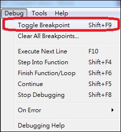
Figure 1: Toggle Breakpoint
Then, you set breakpoint on the left of line number:
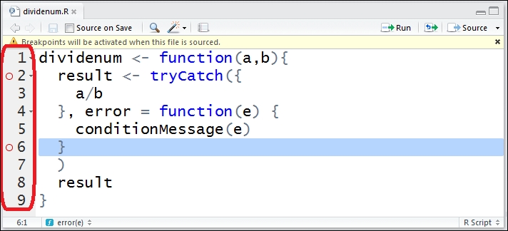
Figure 2: Set breakpoint
Next, you save the code file and click on
Sourceto activate the debugging process: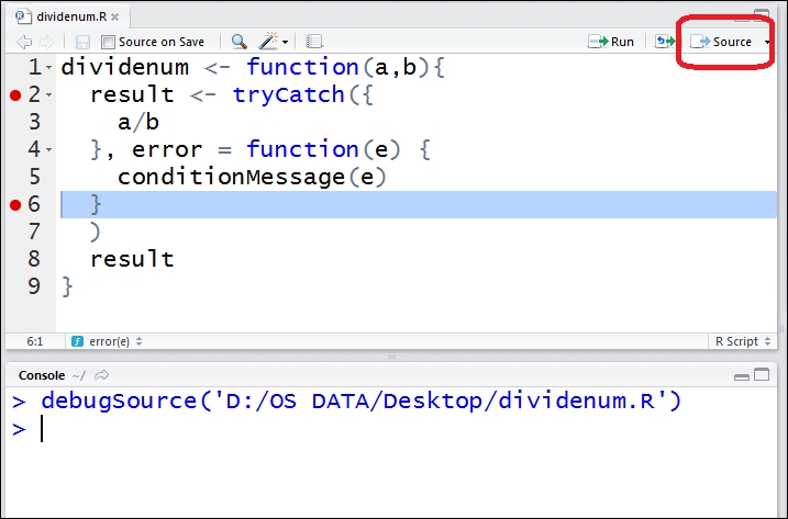
Figure 3: Activate debugging process
Finally, when you invoke the function, your R console will then enter into
Browsemode: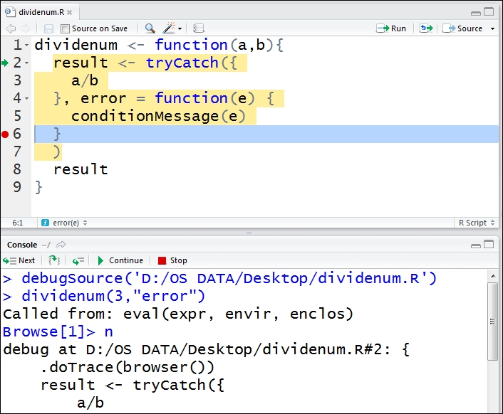
Figure 4: Browse the function
You can now use the command line or dropdown menu of Debug to debug the function:
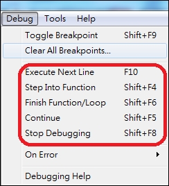
Figure 5: Use debug functions