


1
The Principles of Quantum Mechanics
Quantum mechanics is a framework for the development of physical theories; it is not itself a physical theory [80]. Actual physical theories are built upon a foundation of quantum mechanics. This is why quantum mechanics plays such an important role in all natural sciences. Information theory is no exception and also derives inspiration from the ideas and methods of quantum mechanics.
Understanding quantum computing requires some familiarity with the basic principles of quantum mechanics. This book does not assume any prior knowledge of quantum mechanics and provides all the necessary definitions and explanations when needed. At the same time, the reader is encouraged to learn more about this fascinating subject at the level of mathematical formalism that she is comfortable with. Out of the extensive universe of textbooks on quantum mechanics that provide an introduction to this discipline, it is necessary to mention the classical book by Landau and Lifshitz [182] as well as the equally classical book on quantum computing by Nielsen and Chuang [223], which covers the most relevant aspects of quantum mechanics from the quantum computing perspective. For someone taking their first steps in quantum computing who would like to get the overall picture and some historical perspective, the excellent book by Bernhardt [32] provides both without the heavy usage of complex mathematical apparatus. Readers looking for a more formal modern take on the subject of quantum mechanics may find it in the book by Robinett [249]. The practical aspects of quantum computing are covered in great detail in the book by Sutor [278], and anyone looking for a python quantum computing programming textbook will find it in the work by Loredo [195].
1.1 Linear Algebra for Quantum Mechanics
Quantum computing and quantum mechanics rely on a specific notational formalism, due to Dirac, and are supported by classical linear algebra, in particular Hermitian structures of matrices and tensor products. We provide here a self-contained review of these tools to facilitate the understanding of the rest of the book. We start with basic linear algebra principles before introducing Dirac notations and the quantum counterparts of linear algebra tools. Sections 1.1.1 to 1.1.4 concentrate on standard definitions of finite-dimensional Hilbert spaces and matrices, while Sections 1.1.5 to 1.1.7 review the key details and properties of complex matrices (decompositions, Hermitian property, and rotations). Sections 1.1.9 to 1.1.11 introduce Dirac’s formalism and the essential aspects of quantum operators.
1.1.1 Basic definitions and notations
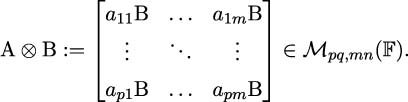
We let 𝔽 denote either the real field ℝ or the complex one ℂ. For a complex number z = x+iy ∈ℂ, with x,y ∈ℝ, we write the conjugate z∗ := x−iy. We let ℳm,n(𝔽) denote the space of matrices of dimension m × n with entries in 𝔽 and ℳn(𝔽) whenever m = n. For A := (aij)1≤i≤m; 1≤j≤n ∈ℳm,n(𝔽), A∗ := (aij∗)1≤i≤m; 1≤j≤n is the complex conjugate. If A ∈ℳn(𝔽), we write A⊤ for its transpose and A† := (A∗)⊤ for its Hermitian conjugate. We finally denote I the identity matrix and write In whenever we wish to emphasise the dimension, and 0m,n the null matrix in ℳm,n(𝔽). Recall that a matrix A ∈ℳn(𝔽) is invertible (or non-singular) if there exists B ∈ℳn(𝔽) such that AB = BA = In. Given two matrices A ∈ℳp,m(𝔽) and B ∈ℳq,n(𝔽), we define their tensor product as
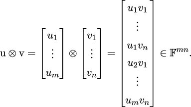
Since a vector is a particular case of a matrix, for u ∈𝔽m and v ∈𝔽n, we can write
1.1.2 Inner products
A vector space V over the field 𝔽 is a set endowed with
- a commutative, associative addition operation,
- an operation of multiplication by a scalar.
The addition and the multiplication by a scalar have the following properties (for scalars α,β ∈𝔽 and vectors u,v ∈V):
- v + 0 = v;
- v + (−v) = 0;
- α(βv) = (αβ)v;
- (α + β)v = αv + βv;
- α(u + v) = αu + αv;
- 1 ⋅ v = v.
Armed with this, we can now define an inner product on V:
Definition 1. A map ⟨⋅,⋅⟩ : V ×V →𝔽 is called an inner product if, for u,v,w ∈V and α ∈𝔽,
- (Positive definiteness) ⟨u,u⟩≥ 0 and ⟨u,u⟩ = 0 if and only if u = 0;
- (Conjugate symmetry) ⟨u,v⟩ = ⟨v,u⟩∗;
- (Linear in the first argument) ⟨u + v,w⟩ = ⟨u,w⟩ + ⟨v,w⟩ and ⟨αu,v⟩ = α⟨u,v⟩;
- (Antilinear in the second argument) ⟨u,v + w⟩ = ⟨u,v⟩ + ⟨u,w⟩ and ⟨u,αv⟩ = α∗⟨u,v⟩.
The inner product is further called non-degenerate if ⟨u,v⟩ = 0 for all v ∈V ∖{0} implies u = 0.
For example, the following spaces carry a natural inner product:
- The vector space ℂn with the inner product ⟨u,v⟩ := u†v = ∑ i=1nui∗vi;
- The space of complex-valued continuous functions on [0,1] with ⟨f,g⟩ := ∫ 01f(t)∗g(t)dt;
- If X,Y ∈ℳm,n(ℝ), then ⟨X,Y⟩ := Tr(X⊤Y) = ∑ i=1m ∑ j=1nXijYij defines an inner product on the space of (real) matrices.
Projection matrices are particularly useful for geometric purposes:
Definition 2. A matrix P ∈ℳn(𝔽) is called a (orthogonal) projection if P2 = P.
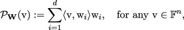
In particular, if W is a vector subspace of 𝔽n with some orthonormal basis (w1,…,wd), it is then easy to check that the map 𝒫W : 𝔽n →𝔽n onto W satisfying
|
defines an orthogonal projection.
1.1.3 From linear operators to matrices
Let V be a finite-dimensional vector space over 𝔽 and ⟨⋅,⋅⟩ a non-degenerate inner product on V. Given a linear operator 𝒜 : V →V, then, by the Riesz representation theorem [309, Section III-6], there exists a unique linear operator 𝒜† : V →V, called the adjoint operator, such that

Indeed, for any v ∈V, the map u ∈V ⟨𝒜u,v⟩ is a linear functional, hence an element of the dual space V† (the space of bounded linear functionals on V), therefore for each v ∈V, there exists v′∈V such that ⟨𝒜u,v⟩ = ⟨u,v′⟩. It is then easy to show that the map v
 v′ is linear, proving that the adjoint operator is uniquely defined. In the particular case where 𝒜 = 𝒜†, the operator 𝒜 is called Hermitian, a key requirement in quantum mechanics:
Definition 3. The operator 𝒜 is called Hermitian, or self-adjoint, if 𝒜 = 𝒜†.
For a Hermitian operator 𝒜, we then have, for any u ∈V,

by conjugate symmetry (Definition 1), and therefore ⟨𝒜u,u⟩ is real. Conversely, if ⟨𝒜u,u⟩ is real, then

Therefore, 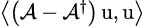 = 0; since this is true for all u ∈V, then 𝒜 = 𝒜†.
The following property of operators shall be useful to ensure that systems driven by operators preserve distances, or norms:
Definition 4. The linear operator 𝒜 : V → V is called unitary if it is surjective and

Recall that a linear operator between two finite-dimensional normed spaces is bounded, and therefore continuous. For any u ∈V, this implies that ∥𝒜u∥ = ∥u∥, so that a unitary operator 𝒜 preserves the norm. In that case, 𝒜 is an isometry, therefore injective. Being also surjective, it is bijective and therefore its inverse exists. For a unitary operator 𝒜 and any u,v ∈V, we have

by definition of the adjoint, implying that
where ℐ is the identity operator.
Example (Real Matrices): If V = ℝn with inner product ⟨u,v⟩ := u⊤v for u,v ∈ℝn, the linear operator 𝒜 can now be viewed as a matrix A in ℳn(ℝ). Its adjoint is nothing other than the transpose A⊤, and therefore A is self-adjoint if and only if it is symmetric. In this case, if A is unitary (or orthogonal), then it is invertible with A−1 = A⊤. Rotation matrices in ℝ2, which will play an important role later when constructing quantum circuits, are the only unitary maps of ℝ2 onto itself and are of the form
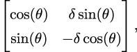
|
for 𝜃 ∈ [0,2π) and δ ∈{−1,+1}.
Example (Complex Matrices): If V = ℂn with inner product ⟨u,v⟩ := v†u for u,v ∈ℂn, the linear operator 𝒜 can now be viewed as a matrix in ℳn(ℂ). The adjoint of such a matrix is then the Hermitian conjugate A† and A is called Hermitian if A = A† and unitary if A†A = In. We shall denote by 𝒰n(ℂ) the set of unitary matrices in ℳn(ℂ). We will discuss Hermitian matrices over ℂ in more detail in Section 1.1.6.
1.1.4 Condition number
In order to manipulate matrices and measure them, we require matrix norms:
Definition 5. A matrix norm ∥⋅∥ : ℳm,n(𝔽) →ℝ is a function satisfying, for any α ∈𝔽 and A,B ∈ℳm,n(𝔽),
- (positively valued) ∥A∥≥ 0;
- (definite) ∥A∥ = 0 if and only if A = 0m,n;
- (absolutely homogeneous) ∥αA∥ = |α|∥A∥;
- (triangle inequality) ∥A + B∥≤∥A∥ + ∥B∥.
The norm is further called sub-multiplicative if ∥AB∥≤∥A∥∥B∥.
The condition number of a matrix is an important tool to understand the stability of linear equations of the form Ax = b, for A ∈ℳn(𝔽), b ∈𝔽n. Assuming A to be non-singular, the true solution is clearly x∗ := A−1b. Suppose, however, that the vector b is only known up to some (not necessarily quantum) measurement error, and one observes instead b + Δb. The solution is then A−1(b + Δb) = x∗ + Δx, with Δx := A−1Δb. In particular, we can write, for any (sub-multiplicative) matrix norm ∥⋅∥,

From this inequality, we see that the quantity ∥A−1∥∥A∥ bounds the relative error in the solution with respect to the relative error in the measurement of the input vector b. This leads to the following terminology:
Definition 6. Given a matrix A ∈ ℳn(𝔽) and a sub-multiplicative norm ∥⋅∥, we call
the condition number (with respect to the norm ∥⋅∥) of the matrix A (and assign to it infinite value if A is singular).
Remark: The definition of the condition number above holds for any matrix norm ∥⋅∥, but admits a more explicit representation in the particular case of the spectral norm ∥⋅∥2, defined as
where ∥x∥2 := 
 is the L 2 norm for vectors. If the matrix A is not singular, then
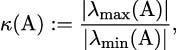
where λmax(A) and λmin(A) denote the largest and smallest eigenvalues of A.
1.1.5 Matrix decompositions and spectral theorem
Having defined essential properties of (complex) matrices, we now introduce several essential tools that allow us to gain a better understanding of their properties.
The Singular Value Decomposition is a key tool to analyse the properties and behaviours of matrices. It is ubiquitous in applied statistics and machine learning and allows us to reduce the explanatory dimension of a large matrix into a small number of meaningful components.
Theorem 1 (Singular Value Decomposition). Let A ∈ℳm,n(𝔽) and p := min(m,n). There exist U ∈𝒰m(𝔽), V ∈𝒰n(𝔽) and σ1 ≥ ≥ σp ≥ 0 such that A = UΣV†, where Σ ∈ℳm,n(𝔽) is diagonal with Σii = σi for i = 1,…,p and Σii = 0 for i > p.
The numbers {σ1,…,σp} are called the singular values of A and are uniquely defined. The columns of U and V are the left-singular and right-singular vectors of A, in the sense that, if σ ∈{σ1,…,σp}, then there exist a column u of U and a column v of V such that Av = σu and A†u = σv. Recall that the rank of a matrix is defined as the dimension of the span of its columns. As a corollary of the Singular Value Decomposition theorem, the rank of a matrix is therefore equal to the number of non-zero singular values. The Singular Value Decomposition is general in the sense that it holds for any matrix. In the particular case of square matrices, the Schur decomposition and the Spectral Theorem provide refinements.
The Spectral Theorem is a cornerstone result in the theory of linear operators, and in particular for (finite-dimensional) matrices. Recall that an operator 𝒜 : V →V is called normal if it commutes with its adjoint, namely if 𝒜𝒜† = 𝒜†𝒜. Self-adjoint (or Hermitian) operators are clearly normal, yet the converse is not true in general. Recall further that an eigenvector of 𝒜 is a non-zero vector u ∈V such that 𝒜u = λu for some λ ∈ℂ, and we denote by σ(𝒜) the set of eigenvalues of 𝒜.
The following result, which is more general than the subsequent spectral theorem, allows us to decompose any arbitrary complex square matrix.
Theorem 2 (Schur Decomposition). For any A ∈ ℳn(ℂ) there exits a unitary matrix U ∈ 𝒰n(ℂ) and an upper triangular matrix T such that A = UTU−1.
Note that since U is unitary, then U−1 = U†. We call the matrix T the Schur transform of A and the identity in the theorem means that A and T are similar, so in particular, possess the same eigenvalues, all located on the diagonal of T. If A is a normal matrix, then so is T, and therefore T must be diagonal and we write T = D for clarity. In this case, we say that the matrix A is diagonalisable with A = UDU†, where the diagonal entries of D are the eigenvalues of A and the column vectors of U are the orthonormal eigenvectors of A.
Theorem 3 (Spectral Theorem). The linear operator 𝒜 : V → V is normal if and only if there exists an orthonormal basis of V consisting of eigenvectors of A.
For each eigenvalue λ ∈ σ(𝒜), denote the corresponding eigenspace

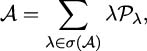
Since the vector space V is the orthogonal direct sum of the eigenspaces (indexed by the eigenvalues of 𝒜), we can then write the spectral decomposition
|
where 𝒫λ is the orthogonal projection operator onto 𝒱λ. Note that such an operator is naturally self-adjoint [309, Theorem 2, Section III-1].
1.1.6 Hermitian matrices
We introduced above Hermitian matrices as the set of matrices A over the complex field ℂ such that A = A†. As fundamental building blocks of quantum computing, we investigate their properties further. Clearly, a real matrix is Hermitian if and only if it is symmetric, in which case A⊤ = A.
Proposition 1. The eigenvalues of a Hermitian matrix are real.
Proof. If Ax = λx for λ ∈ℂ and x ∈ℂn, then
| ⟨Ax,x⟩ | = x†Ax = λx†x = λ∥x∥2, |
| ⟨x,Ax⟩ | = (Ax)†x = (λx)†x = λ∗x†x = λ∗∥x∥2. |
Since both are equal by the Hermitian property, then λ = λ∗, proving the proposition. □
The Singular Value Decomposition (Theorem 1) takes a particular flavour in the case of Hermitian matrices:
Theorem 4. With the notations of Theorem 1, if A ∈ ℳn(ℂ) is Hermitian, then the matrices U and V are equal and the matrix Σ is diagonal with real entries.
Theorem 5. For a Hermitian matrix A ∈ ℳn(ℂ), the following are equivalent:
- The eigenvalues are non-negative.
- There exists a Hermitian matrix B ∈ℳn(ℂ) such that A = B2.
- There exists a matrix B ∈ℳn(ℂ) such that A = B†B.
- For every x ∈ℂn, ⟨Ax,x⟩≥ 0.
Such a matrix is called positive semi-definite.
Proof. The Spectral Theorem shows that there exist a unitary matrix U ∈𝒰n(ℂ) and a diagonal matrix Σ ∈ℳn(ℂ) such that A = UΣU†, where the diagonal elements of Σ are the eigenvalues of A. Assuming (i), we can define B = U U†∈ℳn(ℂ). Then clearly

since U is unitary. The equality A = B†B is also obvious. The latter implies that

Finally, assume (iv) and let λ be an eigenvalue of A with eigenvector u. Then

Since the latter is strictly positive, then clearly λ ≥ 0.
The following property lies at the core of Hamiltonian simulation of quantum systems:
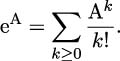
Theorem 6. If A ∈ ℳn(ℂ) is Hermitian, then, for any t ∈ ℝ, eitA is unitary; conversely, every unitary matrix has the form eitA for some Hermitian matrix A.
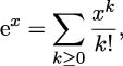
Recall that for a matrix A ∈ℳn(ℂ), its exponential is given by
In practice, though, given a Hermitian matrix A, finding the corresponding unitary matrix U is not easy. The Hamiltonian simulation problem is defined as follows.
Hamiltonian Problem: Given a Hermitian matrix A ∈ℳn(ℂ), a time t > 0, a tolerance level 𝜀 > 0, and some matrix norm ∥⋅∥, find a unitary matrix U such that  ≤ 𝜀.
≤ 𝜀.
1.1.7 Rotation matrices
Rotation matrices, and later their quantum gate equivalents will play a key role in building quantum circuits. Let us start with the following lemma:
Lemma 1. If a matrix A ∈ℳn(ℂ) is such that A2 = I, then for any 𝜃 ∈ℝ,
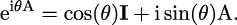
Proof. This follows directly from the series expansion
which has an infinite radius of convergence. □
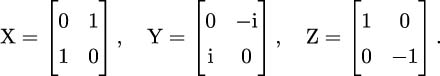
Lemma 1 will prove essential for computational purposes. As simple examples, consider the following:
Exercise: Compute ei𝜃A for A ∈{X,Y,Z} and 𝜃 ∈ℝ, where
For any α ∈ [0,2π), consider now the map ℛα : ℝ2 →ℝ2 such that


which is basically a rotation of angle α and does not affect the norm of the input vector. To the map ℛα, we can associate the (rotation) matrix Rα such that ℛα(u) = Rαu for any u ∈ℝ2. It is easy (exercise) to show the following:
Lemma 2. The matrix Rα has the form
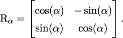
This representation is the general form of a rotation matrix in ℝ2 (introduced in (1.1.3)).
Exercise: Write the matrices ei𝜃A for A ∈{X,Y,Z} from the previous exercise as rotation matrices.
1.1.8 Polar coordinates
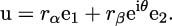
Recall that a point z = x + iy, with x,y ∈ℝ, lying on the unit circle can be written as z = ei𝜃 with 𝜃 ∈ [0,2π). Indeed, simply let x = r cos(𝜃), y = r sin(𝜃) and add the constraint r = 1. Consider now a general vector u ∈ℂ2 of the form
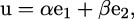
with α,β ∈ℂ such that |α|2 + |β|2 = 1. Here, (e1,e2) forms a basis of ℝ2:
In polar coordinates, we can then write
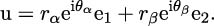
Note that arbitrary multiplication phases have no influence – a fact of key importance in quantum mechanics – because, for any γ ∈ℝ,

so that in fact, multiplying u by the global phase e−i𝜃α and letting 𝜃 := 𝜃β −𝜃α, we consider
Write temporarily rβei𝜃 = x + iy. Insisting on u being on the unit sphere further imposes ∥u∥2 = 1, namely
| 1 | = ∥u∥2 =  rαe1 + (x + iy)e2 rαe1 + (x + iy)e2 † † rαe1 + (x + iy)e2 rαe1 + (x + iy)e2 |
=  rαe1⊤ + (x − iy)e 2⊤ rαe1⊤ + (x − iy)e 2⊤  rαe1 + (x + iy)e2 rαe1 + (x + iy)e2 |
|
| = rα2 + x2 + y2, |
since (e1,e2) is orthonormal. This is nothing more than the equation of the unit sphere. In polar coordinates, we can write

|
and clearly r = 1 since we are on the unit sphere. Therefore
| u | = cos(𝜃)e1 +  sin(𝜃)cos(ϕ) + isin(𝜃)sin(ϕ) sin(𝜃)cos(ϕ) + isin(𝜃)sin(ϕ) e2 e2 |
| = cos(𝜃)e1 + sin(𝜃)eiϕe 2. |
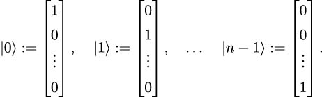
1.1.9 Dirac notations
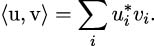
Given a vector v ∈ℂn, Dirac’s ket and bra notations read
![⌊ ⌋ |v1| |v2| |v⟩ := || .|| and ⟨v| := [v∗1,v2∗,...,v∗n]. |⌈ ..|⌉ vn](https://static.packt-cdn.com/products/9781801813570/graphics/media/file53.jpg)
|
With these notations, the operation  := ⟨u|v⟩ defines an inner product on ℂn. The notation for the standard orthonormal basis in ℂn is (
 )i=0,…,n−1, i.e.,
|
In coordinates, we can write, for any u,v ∈ℂn,
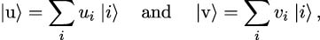
and therefore,
1.1.10 Quantum operators
In the language of Dirac’s notations, we can define the outer product  ⟨v| (for u ∈U and v ∈V) as a linear operator from V to U, two vector spaces, as

|
In particular,  ⟨v| is the projection on the one-dimensional space generated by
  . Any linear operator can be expressed as a linear combination of outer products as
|
where  and
and  are the standard basis vectors (1.1.9).
Similarly to the linear algebra setting above, we can define an eigenvector of a linear operator 𝒜 : V →V as a non-zero vector  such that
|
for some complex eigenvalue λ. Associated with any linear operator 𝒜, the adjoint operator 𝒜† satisfies
|
Indeed, in the language of linear operators above, we have

by definition of the inner product (Definition 1).
1.1.11 Tensor product
Given two vector spaces U and V of dimensions m and n, the tensor product U ⊗V is a vector space of dimension mn. For u ∈U and v ∈V, we can form the vector  :=
:=  ⊗
⊗ ∈U ⊗V with the following properties:
 =
=  +
+  , for any u′∈U;
 =
=  +
+  , for any v′∈V;
- α
 =
=  =
=  , for any α ∈ℂ.
Given the linear operators 𝒜 : U →U and ℬ : V →V, we can then define their tensor product as an operator 𝒜⊗ℬ on U ⊗V:
|
which can be represented in matrix form as A ⊗ B ∈ℳmn,mn(ℂ).
This Dirac formalism, fully anchored in (classical) linear algebra, now opens the gates to a proper dive into the foundations of quantum mechanics.
1.2 Postulates of Quantum Mechanics
Quantum mechanics states several mathematical postulates that a physical theory must satisfy. It turns out that the mathematics of quantum mechanics allows for more general computation: more general definition of the memory state in comparison with classical digital computing and a wider range of possible transformations of such memory states. A natural question arises: what is the reason for this superior mode of computation not being used until very recently? The answer is that although quantum mechanics was formulated almost a century ago (Paul Dirac’s seminal work "The Principles of Quantum Mechanics" [86] was published in 1930), the realisation of the rules of quantum mechanics in the computational protocol performed on classical digital computers requires an enormous amount of memory. Exponential gains in computing power are offset by exponential memory requirements.
In order to perform quantum computations efficiently, we need to use actual quantum mechanical systems, with their ability to encode information in their states. To illustrate this point, the state of a quantum system consisting of n quantum bits (qubits) can be described by specifying 2n probability amplitudes – this is a huge amount of information even for very small systems (n ∼ 100) and it would be impossible to store this information in classical memory. It took decades of technological progress before quantum processing units (QPUs) – devices that control quantum mechanical systems performing computations – became feasible.
Let us now proceed with the formulation of the mathematical postulates that lie at the foundation of quantum mechanics. These postulates specify a general framework for describing the behaviour of a physical system [80, 182, 249]:
- How to describe the state of a closed system.
- How to describe the evolution of a closed system.
- How to describe the interactions of a system with external systems.
- How to describe observables of a system.
- How to describe the state of a composite system in terms of its component parts.
1.2.1 First postulate – Statics
Postulate 1. Associated to any physical system is a complex inner product space known as the state space of the system. The system is completely described at any given point in time by its state vector, which is a unit vector in its state space.
What is the importance of the first postulate from the quantum computing point of view? The answer is that quantum mechanics offers us a straightforward generalisation of the classical binary digit (bit). The classical bit is a two-state system with controlled transitions between them. As an example, we can use an electrical switch that can exist in one of the two discrete, stable states ("on" and "off"). Although electrical switches may seem an odd physical realisation of bits in the age of transistors, they illustrate an important point about computation in general: it is substrate independent. Exactly the same computational results can be obtained using electrical relays and CMOS transistors.
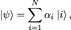
The quantum mechanical version of a bit, called a quantum binary digit (qubit), is a quantum mechanical two-state system. The first postulate of quantum mechanics tells us that the state of such a system can be represented mathematically by a unit vector in the two-dimensional complex vector space. This also means that such a system can exist in a superposition of basis states. Indeed, any vector  in the two-dimensional complex vector space,

can be represented as a linear combination of the standard basis vectors:

Since the state vector is a unit vector, the coefficients α and β must satisfy

The coefficients α and β are probability amplitudes. Even though a qubit can exist in a superposition of basis states, once measured (see Postulate 3), its state collapses to one of the basis states: |α|2 and |β|2 give us the probability of finding the qubit, respectively, in states  and
and  after measurement.
One can draw an analogy with how the space of natural numbers, ℕ, can be extended to the space of real numbers, ℝ, and then to the space of complex numbers, ℂ. We have a much wider range of functions that can operate on and take values in ℝ and ℂ than in ℕ. Similarly, allowing the two-state system to exist in a superposition of states significantly extends the range of possible operators that can transform such states (i.e., perform computation).
For example, there is no Boolean function f that, when applied twice to a classical bit, would result in a NOT gate: f(f(0)) = 1 and f(f(1)) = 0. But there is such an operator in quantum computing. We can easily verify by direct calculations that the matrix

applied twice to the basis vector  would transform it to the basis vector
  , and applied twice to the basis vector
  would transform it to the basis vector
  . M is an example of a quantum logic gate – an operator that transforms the state of a qubit, thus implementing the computation.
Remark: The state space of a physical system can be infinite-dimensional. The quantum computing paradigm based on infinite-dimensional Hilbert spaces is called continuous-variable quantum computing, which is realised in, e.g., some photonic quantum computing systems. However, in the context of digital quantum computing, we will restrict our analysis to finite-dimensional state spaces.
The state of a qubit (the fundamental memory unit of quantum computing that generalises the concept of a classical bit) can be described mathematically as a unit vector in the two-dimensional complex vector space. Any physical system whose state space can be described by ℂ2 can serve as an implementation of a qubit.
1.2.2 Second postulate – Dynamics
Postulate 2. The time evolution of a closed quantum system is described by the Schrödinger equation

|
where ℏ is Planck’s constant and ℋ is a time-independent Hermitian operator known as the Hamiltonian of the system.
The Hamiltonian of a quantum system is an operator corresponding to the total energy of that system, and its eigenvalues are the possible energy levels of the system. The knowledge of the Hamiltonian provides all the necessary information about system dynamics.
In the Schrödinger equation (1.2.2), the state  of a closed quantum system at time t1 is related to the state
  at time t2 by a unitary operator 𝒰(t1,t2) that depends only on t1 and t2 via

|
where 𝒰(t1,t2) is obtained from the Hamiltonian ℋ as

|
Unitary operators preserve the inner product (and therefore norms, lengths, and distances), which means that for two vectors  and
and  , if 𝒰 is a unitary operator, then the inner product between 𝒰
 and 𝒰
and 𝒰 is the same as the inner product between
  and
and  :
:

|
A unitary operator is a complex generalisation of a rotation: unitary operators take an orthonormal basis to another orthonormal basis, and any operator with this property is unitary. In quantum mechanics, physical transformations such as rotations, translations and time evolution correspond to maps that take quantum states to other quantum states. These maps should be linear and preserve the inner product. This allows us to look at the unitary operators as the quantum logic gates implementing quantum computation protocols. Furthermore, unitary operators are invertible, a key property that ensures that quantum computing is reversible.
Quantum logic gates (quantum counterparts of the Boolean logic gates in classical computing) are unitary operators that transform quantum states, thus implementing the computation.
1.2.3 Third postulate – Measurement
Given a Hermitian operator 𝒜, the spectral theorem implies that the state  of a system can be written as a superposition

|
where the coefficients (αi)i=1,…,N are complex probability amplitudes, assumed to be normalised with ∑ i=1N|αi|2 = 1, and where ( )i=1,…,N are eigenfunctions of 𝒜. The measurement postulate then reads as follows:
Postulate 3. If we measure the Hermitian operator 𝒜 in the state  given in (1.2.3), the possible outcomes for the measurement are the eigenvalues (λi)i=1,…,N of 𝒜, and the probability pi to measure λi is given by pi = |αi|2. After the outcome λi, the state of the system becomes

|
An immediate measurement in the same computational basis will deliver the same result without any uncertainty.
The quantum measurements are described by measurement operators (𝒫i)i=1,…,N, acting on the state space of the system with N possible outcomes. If the state of the system is  before the measurement, then the probability of outcome i is

The measurement operators should also satisfy the completeness condition

|
where ℐ is the identity operator. This ensures that the sum of the probabilities of all outcomes adds up to 1.
These measurement operators are linear but not unitary. From the quantum computing perspective, we are interested in measurement operators that are projections (Definition 2) onto the computational basis, such as the standard orthonormal basis given by (1.1.9).
For example, the measurement operators for a single qubit can be defined as

We can easily verify that 𝒫02 = 𝒫0 and 𝒫12 = 𝒫1, as should be the case for projection operators, and that the completeness condition (1.2.3) is satisfied. If the qubit is in state  = α
= α + β
+ β , then the measurement operator 𝒫0 will give us
  with probability |α|2, and the measurement operator 𝒫1 will give us
  with probability |β|2. Indeed,
𝒫0 |
=  ⟨0| ⟨0| α α + β + β  = α = α ⟨0| ⟨0| + β + β ⟨0| ⟨0| = α = α , , |
𝒫1 |
=  ⟨1| ⟨1| α α + β + β  = α = α ⟨1| ⟨1| + β + β ⟨1| ⟨1| = β = β . . |
The measurement postulate of quantum mechanics states that an immediate measurement in the same computational basis will deliver the same result without any uncertainty. The key words here are "the same computational basis". What would happen if the subsequent measurement is performed in another basis (the basis specified by another set of linearly independent unit vectors from the state space)? For example, assume that the qubit is in state

Measuring  in {
in { ,
, } computational basis will result in observing states
  and
and  with equal probability 1∕2. Let us assume that we measured
  . The qubit state is now

If we repeat the measurement in the same { ,
, } computational basis, we obtain state
  with probability 1 in accordance with the measurement postulate. However, had we measured state
  in the Hadamard basis {
 ,
, }, given by

|
we would have equal probabilities of  and
and  outcomes. Let us assume that we measured
  and the state of the qubit is now

If we repeat the measurement of state  in the Hadamard basis {
 ,
, }, we obtain state
  with probability 1. But the state of the qubit is an equal superposition of states
  and
and  from the {
 ,
, } computational basis perspective and we have an equal chance of measuring either
  or
or  in this basis.
Remark: The basis vectors  and
and  that form the standard computational basis can be transformed into the basis vectors
  and
and  that form the Hadamard basis by applying the following unitary operator (rotation), called the Hadamard gate:

|
Chapters 6, 10 and 11 provide examples of applications of the Hadamard gate.
The measurement plays a crucial role in quantum computing. This is the process of collapsing a quantum state and reading out the classical information: measuring qubits encoding a quantum state will produce a classical bit string. The measurement process generates probabilistic outcomes. Therefore, we need to perform measurements on the same quantum state multiple times to generate a sufficiently large number of classical bit strings to produce reliable statistics.
The process of measurement describes the collapse of the quantum state due to contact with the environment. After measurement, the states of the qubits are known without any uncertainty. It is possible to extract at most 1 bit of information from a qubit. In order to extract more information about the probability distribution encoded in a given quantum state, it is necessary to perform measurement of the same state multiple times.
1.2.4 Fourth postulate – Observable
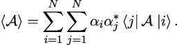
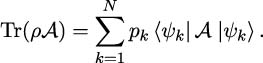
Postulate 4. For every measurable property of a physical system, there exists a corresponding Hermitian operator. The values of the physical observables correspond to the expectation values of Hermitian operators. The expectation value  of the Hermitian operator 𝒜 in the normalised state
  is given by

|
Let us consider the general case where the expectation value of a Hermitian operator 𝒜 is calculated in state  , which is not an eigenfunction of 𝒜. By the Spectral Theorem 3 (see also (1.2.3)), the state
  of a system can be represented as the superposition

where ( )i=1,…,N are the eigenfunctions of 𝒜 and (αi)i=1,…,N the corresponding probability amplitudes.
Therefore, the expectation value of 𝒜 in state  , given in (1.2.4), is calculated as

where (λi)i=1,…,N are the eigenvalues of 𝒜. The only terms that survive in the expression for  are those with i = j due to the orthogonality of the eigenfunctions, so that

Therefore, the value of the observable is a weighted average of the eigenvalues of the corresponding Hermitian operator. The weights are the coefficients (|αi|2)i=1,…,N, which are the probabilities of measuring the corresponding eigenstate of 𝒜.
Hermitian operators play an exceptionally important role in quantum mechanics since their expectation values correspond to physical observables.
1.2.5 Fifth postulate – Composite System
Postulate 5. The state space of a composite physical system is the tensor product of the state spaces of the individual component physical systems.
If the first component physical system is in state  and the second component physical system is in state
  , then the state of the combined system,
  , is given by the tensor product

|
Not all states of a combined system can be separated into the tensor product of states of individual components. If the state of a system cannot be separated into component parts, we say that the component parts are entangled.
The entanglement of quantum systems is one of the major sources of computational power of quantum computing. It allows us to store exponentially more information in the correlations between the states of individual subsystems (in the limit – individual qubits) than directly in the states of individual subsystems.
To illustrate this point, we can look at the number of probability amplitudes needed to describe the state of an n-qubit system. An individual qubit can be found in one of the two possible states after measurement – one of the two basis states,  or
or  . This means that we need to specify two probability amplitudes to fully describe the state of the qubit before measurement. If all our qubits are independent and the state of the system can be represented as a tensor product of individual qubit states,

|
then we need to specify 2n probability amplitudes (two for each individual quantum states) to describe the state  of the system. If, however, all individual qubits are entangled and the tensor product representation of the system state
  does not exist, we need to specify 2n probability amplitudes – this is an effective measure of useful information that can be stored in the system.
The power of quantum computing is derived from the principles of superposition and entanglement. Entanglement allows us to store most of the information in correlations between the qubit states.
1.3 Pure and Mixed States
There are situations where the state of a quantum mechanical system cannot be described with the help of a state vector. Here, we look at such situations and provide a mathematical tool for describing them.
1.3.1 Density matrix
Let us start with the state of a combined two-component physical system given by (1.2.5). Let ( )i=1,...,N and (
 )j=1,...,M denote, respectively, the standard orthonormal bases of the Hilbert spaces of systems A and B:
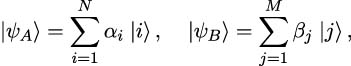
|
where (αi)i=1,...,N and (βj)j=1,...,M are some probability amplitudes. The states that allow the state vector representation (1.3.1) are called pure states. In this case, the state of the combined system is
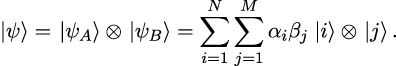
|
However, in general, the state of the combined system would look like
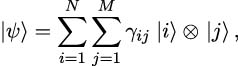
|
where γij are probability amplitudes that may not necessarily be factorised as the product of probability amplitudes (αi)i=1,...,N and (βj)j=1,...,M. If γij cannot be factorised as αiβj, then the component systems A and B are entangled and their states cannot be represented by the state vectors (1.3.1). Such states of systems A and B are called mixed states.
The more general setup is that of an ensemble of states of the form {pk, }k=1,…,N, where each
  is a quantum state whose wavefunction is known with certainty (although this does not necessarily provide full knowledge of the measurement statistics), and each pk is the associated probability (not amplitude) in [0,1]. In order to define properly pure and mixed states, introduce the density operator as follows:
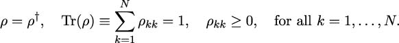
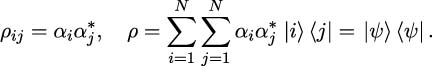
Definition 7. A density operator ρ is a positive semidefinite Hermitian operator with unit trace and takes the form
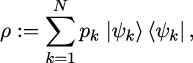
|
where ∑ k=1Npk = 1 and  equals 1 if k = l and zero otherwise.
Mathematically, such a density operator ρ corresponds to a density matrix (ρkl)k,l=1,…,N such that
1.3.2 Pure state
A pure state is one that can be represented by a state vector
|
where (αi)i=1,...,N are probability amplitudes in ℂ such that ∑ i=1N|αi|2 = 1. In the ensemble setup above, this means that there exists k∗∈{1,…,N} such that pk∗ = 1 and hence  =
=  and therefore ρ =
  ⟨ψ|. The density matrix also allows us to compute expectations of the form (1.2.4):
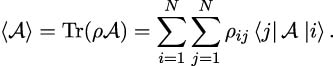
Lemma 3. Let ρ be the density matrix associated to the pure state (1.3.2) and let 𝒜 be an observable (Hermitian operator), then

Proof. The lemma follows from the immediate computation
⟨ψ|𝒜 |
= ⟨ψ|𝒜∑ i=1Nα i |
= ∑ i=1Nα i ⟨ψ|𝒜 |
|
= ∑ i=1N ⟨ψ|𝒜 ⟨ψ|𝒜 |
|
= ∑ i=1N ⟨i|ρ𝒜 = Tr(ρ𝒜). = Tr(ρ𝒜). |
With the state  given by (1.3.2), we obtain
|
At the same time we have
|
Comparison of (1.3.2) and (1.3.2) yields the following expression for the density matrix of a pure state:
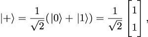
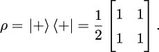
Example: An example of a pure state is the Hadamard state
with corresponding density matrix
1.3.3 Mixed state
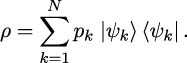
A mixed state is one that cannot be represented by a single pure state vector, and is therefore represented as a statistical distribution of pure states in the form of an ensemble of quantum states {pk, }k=1,…,N, where ∑ k=1Npk = 1 and pk ∈ [0,1] for each k. The density of a mixed state therefore reads
|
Similarly to Lemma 3, we can write expectations of observables with respect to mixed states using the density matrix:
Lemma 4. Let ρ be the density matrix associated to the mixed state (1.3.3) and let 𝒜 be an observable (Hermitian operator), then
Proof. The lemma follows from the immediate computation
| Tr(ρ𝒜) | = ∑ i=1N ⟨i|ρ𝒜 |
= ∑ i=1N ⟨i|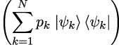 𝒜 𝒜 |
|
= ∑ k=1Np k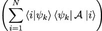 |
|
= ∑ k=1Np k ⟨ψk|𝒜 . . |
Let us see now how the density matrix formalism can help us describe the state of a combined system. Consider an entangled state of two systems, A and B, given by (1.3.1), and a Hermitian operator 𝒜 that only acts within the Hilbert space of system A. What would be the expectation value of 𝒜 in this state? Starting with (1.2.4), we obtain
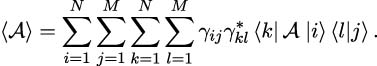
|
Since only terms with l = j survive in (1.3.3) due to the orthogonality of the basis states, we have
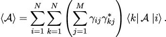
|
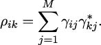
Thus, the density matrix that describes the mixed state of system A is
Note that in the case where the probability amplitudes γij can be factorised as the product of probability amplitudes (αi)i=1,...,N and (βj)j=1,...,M, we obtain
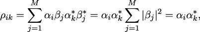
which describes a pure state.
A simple criterion to distinguish a pure state from a mixed state is the following:
Lemma 5. Let ρ be a density matrix. The inequality Tr(ρ2) ≤ 1 always holds and Tr(ρ2) = 1 if and only if ρ corresponds to a pure state.
Proof. Consider an ensemble of pure states {pi, }i=1,…,N, with density matrix given by (1.3.3). Therefore
| Tr(ρ2) | = Tr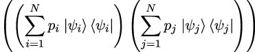 |
= Tr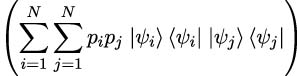 |
|
= Tr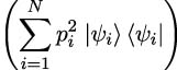 = ∑ i=1Np i2Tr = ∑ i=1Np i2Tr  ⟨ψi| ⟨ψi| = ∑ i=1Np i2 = ∑ i=1Np i2 = ∑ i=1Np i2, = ∑ i=1Np i2, |
which is smaller than 1 since the pi are probabilities in [0,1] summing up to 1. Assume now that Tr(ρ2) equals one, then so does ∑ i=1Npi2. If pi ∈ (0,1) for all i = 1,…,N, then
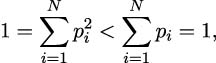
which is a contradiction, and therefore there exists i∗∈{1,…,N} such that pi∗ = 1, so that ρ =  ⟨ψi∗| is a pure state. Conversely, if ρ =
  ⟨ψi| for some i ∈{1,…,N} represents a pure state, then

Example: An example of a mixed state is a statistical ensemble of states  and
and  . If a physical system is prepared to be either in state
  or state
  with equal probability, it can be described by the mixed state
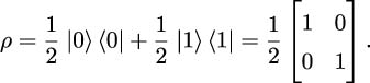
|
Note that this is different from the density matrix of the pure state
which reads

Unlike pure quantum states, mixed quantum states cannot be described by a single state vector. However, the pure states and the mixed states can be described by the density matrix.
Summary
In this chapter, we learned the key principles of quantum mechanics, starting with a review of the basic elements of linear algebra, followed by an introduction to Dirac notations.
We then covered the main postulates of quantum mechanics and their relevance to quantum computing. We learned how to describe the state (statics) and the evolution (dynamics) of a closed system, the interactions of a system with external systems (measurement), observables, as well as the state of a composite system in terms of its component parts.
We finally introduced the density operator, which allows us to describe both pure and mixed quantum states, contrasting with the state vector, which can only represent pure quantum states.
In the next chapter, we will look at an application of the principles of quantum mechanics to analog quantum computing – quantum annealing.
Join our book’s Discord space
Join our Discord community to meet like-minded people and learn alongside more than 2000 members at: https://packt.link/quantum

