In this chapter, we will cover:
- Importing nonspatial tabular data (CSV) using PostGIS functions
- Importing nonspatial tabular data (CSV) using GDAL
- Importing shapefiles with shp2pgsql
- Importing and exporting data with the ogr2ogr GDAL command
- Handling batch importing and exporting of datasets
- Exporting data to a shapefile with the pgsql2shp PostGIS command
- Importing OpenStreetMap data with the osm2pgsql command
- Importing raster data with the raster2pgsql PostGIS command
- Importing multiple rasters at a time
- Exporting rasters with the gdal_translate and gdalwarp GDAL commands
PostGIS is an open source extension for the PostgreSQL database that allows support for geographic objects; throughout this book you will find recipes that will guide you step by step to explore the different functionalities it offers.
The purpose of the book is to become a useful tool for understanding the capabilities of PostGIS and how to apply them in no time. Each recipe presents a preparation stage, in order to organize your workspace with everything you may need, then the set of steps that you need to perform in order to achieve the main goal of the task, that includes all the external commands and SQL sentences you will need (which have been tested in Linux, Mac and Windows environments), and finally a small summary of the recipe. This book will go over a large set of common tasks in geographical information systems and location-based services, which makes it a must-have book in your technical library.
In this first chapter, we will show you a set of recipes covering different tools and methodologies to import and export geographic data from the PostGIS spatial database, given that pretty much every common action to perform in a GIS starts with inserting or exporting geospatial data.
There are a couple of alternative approaches to importing a Comma Separated Values (CSV) file, which stores attributes and geometries in PostGIS. In this recipe, we will use the approach of importing such a file using the PostgreSQL COPY command and a couple of PostGIS functions.
We will import the firenews.csv file that stores a series of web news collected from various RSS feeds related to forest fires in Europe in the context of the European Forest Fire Information System (EFFIS), available at http://effis.jrc.ec.europa.eu/.
For each news feed, there are attributes such as place name, size of the fire in hectares, URL, and so on. Most importantly, there are the x and y fields that give the position of the geolocalized news in decimal degrees (in the WGS 84 spatial reference system, SRID = 4326).
For Windows machines, it is necessary to install OSGeo4W, a set of open source geographical libraries that will allow the manipulation of the datasets. The link is: https://trac.osgeo.org/osgeo4w/
In addition, include the OSGeo4W and the Postgres binary folders in the Path environment variable to be able to execute the commands from any location in your PC.
The steps you need to follow to complete this recipe are as shown:
- Inspect the structure of the CSV file,
firenews.csv, which you can find within the book dataset (if you are on Windows, open the CSV file with an editor such as Notepad).
      $ cd ~/postgis_cookbook/data/chp01/
      $ head -n 5 firenews.csv
The output of the preceding command is as shown:

- Connect to PostgreSQL, create the
chp01 SCHEMA, and create the following table:
      $ psql -U me -d postgis_cookbook
      postgis_cookbook=> CREATE EXTENSION postgis;
      postgis_cookbook=> CREATE SCHEMA chp01;
      postgis_cookbook=> CREATE TABLE chp01.firenews
      (
        x float8,
        y float8,
        place varchar(100),
        size float8,
        update date,
        startdate date,
        enddate date,
        title varchar(255),
        url varchar(255),
        the_geom geometry(POINT, 4326)
      );
Note
We are using the psql client for connecting to PostgreSQL, but you can use your favorite one, for example, pgAdmin.
Using the psql client, we will not show the host and port options as we will assume that you are using a local PostgreSQL installation on the standard port.
If that is not the case, please provide those options!
      postgis_cookbook=> COPY chp01.firenews (
        x, y, place, size, update, startdate,
        enddate, title, url
      ) FROM '/tmp/firenews.csv' WITH CSV HEADER;
Note
Make sure that the firenews.csv file is in a location accessible from the PostgreSQL process user. For example, in Linux, copy the file to the /tmp directory.
If you are on Windows, you most likely will need to set the encoding to UTF-8 before copying: postgis_cookbook=# set client_encoding to 'UTF-8'; and remember to set the full path, 'c:\\tmp\firenews.csv'.
- Check all of the records have been imported from the CSV file to the PostgreSQL table:
postgis_cookbook=> SELECT COUNT(*) FROM chp01.firenews;The output of the preceding command is as follows:

- Check a record related to this new table is in the PostGIS
geometry_columnsmetadata view:
     postgis_cookbook=# SELECT f_table_name,
     f_geometry_column, coord_dimension, srid, type
     FROM geometry_columns where f_table_name = 'firenews';
The output of the preceding command is as follows:

Note
Before PostGIS 2.0, you had to create a table containing spatial data in two distinct steps; in fact, the geometry_columns view was a table that needed to be manually updated. For that purpose, you had to use the AddGeometryColumn function to create the column. For example, this is for this recipe:postgis_cookbook=> CREATE TABLE chp01.firenews(x float8,y float8,place varchar(100),size float8,update date,startdate date,enddate date,title varchar(255),url varchar(255))WITHOUT OIDS;postgis_cookbook=> SELECT AddGeometryColumn('chp01', 'firenews', 'the_geom', 4326, 'POINT', 2);chp01.firenews.the_geom SRID:4326 TYPE:POINT DIMS:2
In PostGIS 2.0, you can still use the AddGeometryColumn function if you wish; however, you need to set its use_typmod parameter to false.
      postgis_cookbook=> UPDATE chp01.firenews
      SET the_geom = ST_SetSRID(ST_MakePoint(x,y), 4326);
      postgis_cookbook=> UPDATE chp01.firenews
      SET the_geom = ST_PointFromText('POINT(' || x || ' ' || y || ')',
                                      4326);
- Check how the geometry field has been updated in some records from the table:
      postgis_cookbook=# SELECT place, ST_AsText(the_geom) AS wkt_geom
      FROM chp01.firenews ORDER BY place LIMIT 5;
The output of the preceding comment is as follows:

- Finally, create a spatial index for the geometric column of the table:
      postgis_cookbook=> CREATE INDEX idx_firenews_geom
      ON chp01.firenews USING GIST (the_geom);
This recipe showed you how to load nonspatial tabular data (in CSV format) in PostGIS using the COPY PostgreSQL command.
After creating the table and copying the CSV file rows to the PostgreSQL table, you updated the geometric column using one of the geometry constructor functions that PostGIS provides (ST_MakePoint and ST_PointFromText for bi-dimensional points).
These geometry constructors (in this case, ST_MakePoint and ST_PointFromText) must always provide the spatial reference system identifier (SRID) together with the point coordinates to define the point geometry.
Each geometric field added in any table in the database is tracked with a record in the geometry_columns PostGIS metadata view. In the previous PostGIS version (< 2.0), the geometry_fields view was a table and needed to be manually updated, possibly with the convenient AddGeometryColumn function.
For the same reason, to maintain the updated geometry_columns view when dropping a geometry column or removing a spatial table in the previous PostGIS versions, there were the DropGeometryColumn and DropGeometryTable functions. With PostGIS 2.0 and newer, you don't need to use these functions any more, but you can safely remove the column or the table with the standard ALTER TABLE, DROP COLUMN, and DROP TABLE SQL commands.
In the last step of the recipe, you have created a spatial index on the table to improve performance. Please be aware that as in the case of alphanumerical database fields, indexes improve performances only when reading data using the SELECT command. In this case, you are making a number of updates on the table (INSERT, UPDATE, and DELETE); depending on the scenario, it could be less time consuming to drop and recreate the index after the updates.
As an alternative approach to the previous recipe, you will import a CSV file to PostGIS using the ogr2ogr GDAL command and the GDAL OGR virtual format. The Geospatial Data Abstraction Library (GDAL) is a translator library for raster geospatial data formats. OGR is the related library that provides similar capabilities for vector data formats.
This time, as an extra step, you will import only a part of the features in the file and you will reproject them to a different spatial reference system.
You will import the Global_24h.csv file to the PostGIS database from NASA's Earth Observing System Data and Information System (EOSDIS).
You can copy the file from the dataset directory of the book for this chapter.
This file represents the active hotspots in the world detected by the Moderate Resolution Imaging Spectroradiometer (MODIS) satellites in the last 24 hours. For each row, there are the coordinates of the hotspot (latitude, longitude) in decimal degrees (in the WGS 84 spatial reference system, SRID = 4326), and a series of useful fields such as the acquisition date, acquisition time, and satellite type, just to name a few.
You will import only the active fire data scanned by the satellite type marked as T (Terra MODIS), and you will project it using the Spherical Mercator projection coordinate system (EPSG:3857; it is sometimes marked as EPSG:900913, where the number 900913 represents Google in 1337 speak, as it was first widely used by Google Maps).
The steps you need to follow to complete this recipe are as follows:
- Analyze the structure of the
Global_24h.csvfile (in Windows, open the CSV file with an editor such as Notepad):
      $ cd ~/postgis_cookbook/data/chp01/
      $ head -n 5 Global_24h.csv
The output of the preceding command is as follows:

- Create a GDAL virtual data source composed of just one layer derived from the
Global_24h.csvfile. To do so, create a text file namedglobal_24h.vrtin the same directory where the CSV file is and edit it as follows:
       <OGRVRTDataSource>
         <OGRVRTLayer name="Global_24h">
         <SrcDataSource>Global_24h.csv</SrcDataSource>
         <GeometryType>wkbPoint</GeometryType>
         <LayerSRS>EPSG:4326</LayerSRS>
           <GeometryField encoding="PointFromColumns"
            x="longitude" y="latitude"/>
         </OGRVRTLayer>
</OGRVRTDataSource> $ ogrinfo global_24h.vrt Global_24h -fid 1The output of the preceding command is as follows:

You can also try to open the virtual layer with a desktop GIS supporting a GDAL/OGR virtual driver such as Quantum GIS (QGIS). In the following screenshot, the Global_24h layer is displayed together with the shapefile of the countries that you can find in the dataset directory of the book:

The global_24h dataset over the countries layers and information of the selected features
- Now, export the virtual layer as a new table in PostGIS using the
ogr2ogrGDAL/OGR command (in order for this command to become available, you need to add the GDAL installation folder to thePATHvariable of your OS). You need to use the-foption to specify the output format, the-t_srsoption to project the points to theEPSG:3857spatial reference, the-whereoption to load only the records from the MODIS Terra satellite type, and the-lcolayer creation option to provide the schema where you want to store the table:
      $ ogr2ogr -f PostgreSQL -t_srs EPSG:3857
      PG:"dbname='postgis_cookbook' user='me' password='mypassword'"
      -lco SCHEMA=chp01 global_24h.vrt -where "satellite='T'"
      -lco GEOMETRY_NAME=the_geom
- Check how the
ogr2ogrcommand created the table, as shown in the following command:
      $ pg_dump -t chp01.global_24h --schema-only -U me postgis_cookbook

      CREATE TABLE global_24h (
        ogc_fid integer NOT NULL,
        latitude character varying,
        longitude character varying,
        brightness character varying,
        scan character varying,
        track character varying,
        acq_date character varying,
        acq_time character varying,
        satellite character varying,
        confidence character varying,
        version character varying,
        bright_t31 character varying,
        frp character varying,
        the_geom public.geometry(Point,3857)
);- Now, check the record that should appear in the
geometry_columnsmetadata view:
      postgis_cookbook=# SELECT f_geometry_column, coord_dimension,
      srid, type FROM geometry_columns
      WHERE f_table_name = 'global_24h';
The output of the preceding command is as follows:

- Check how many records have been imported in the table:
postgis_cookbook=# SELECT count(*) FROM chp01.global_24h;The output of the preceding command is as follows:

- Note how the coordinates have been projected from
EPSG:4326toEPSG:3857:
      postgis_cookbook=# SELECT ST_AsEWKT(the_geom)
      FROM chp01.global_24h LIMIT 1;
The output of the preceding command is as follows:

As mentioned in the GDAL documentation:
"OGR Virtual Format is a driver that transforms features read from other drivers based on criteria specified in an XML control file."
GDAL supports the reading and writing of nonspatial tabular data stored as a CSV file, but we need to use a virtual format to derive the geometry of the layers from attribute columns in the CSV file (the longitude and latitude coordinates for each point). For this purpose, you need to at least specify in the driver the path to the CSV file (the SrcDataSource element), the geometry type (the GeometryType element), the spatial reference definition for the layer (the LayerSRS element), and the way the driver can derive the geometric information (the GeometryField element).
There are many other options and reasons for using OGR virtual formats; if you are interested in developing a better understanding, please refer to the GDAL documentation available at http://www.gdal.org/drv_vrt.html.
After a virtual format is correctly created, the original flat nonspatial dataset is spatially supported by GDAL and software-based on GDAL. This is the reason why we can manipulate these files with GDAL commands such as ogrinfo and ogr2ogr, and with desktop GIS software such as QGIS.
Once we have verified that GDAL can correctly read the features from the virtual driver, we can easily import them in PostGIS using the popular ogr2ogr command-line utility. The ogr2ogr command has a plethora of options, so refer to its documentation at http://www.gdal.org/ogr2ogr.html for a more in-depth discussion.
In this recipe, you have just seen some of these options, such as:
-where: It is used to export just a selection of the original feature class-t_srs: It is used to reproject the data to a different spatial reference system-lco layer creation: It is used to provide the schema where we would want to store the table (without it, the new spatial table would be created in thepublicschema) and the name of the geometry field in the output layer
If you need to import a shapefile in PostGIS, you have at least a couple of options such as the ogr2ogr GDAL command, as you have seen previously, or the shp2pgsql PostGIS command.
In this recipe, you will load a shapefile in the database using the shp2pgsql command, analyze it with the ogrinfo command, and display it in QGIS desktop software.
The steps you need to follow to complete this recipe are as follows:
- Create a shapefile from the virtual driver created in the previous recipe using the
ogr2ogrcommand (note that in this case, you do not need to specify the-foption as the shapefile is the default output format for theogr2ogrcommand):
$ ogr2ogr global_24h.shp global_24h.vrt- Generate the SQL dump file for the shapefile using the
shp2pgsqlcommand. You are going to use the-Goption to generate a PostGIS spatial table using the geography type, and the-Ioption to generate the spatial index on the geometric column:
      $ shp2pgsql -G -I global_24h.shp
chp01.global_24h_geographic > global_24h.sql- Analyze the
global_24h.sqlfile (in Windows, use a text editor such as Notepad):
$ head -n 20 global_24h.sqlThe output of the preceding command is as follows:

- Run the
global_24h.sqlfile in PostgreSQL:
$ psql -U me -d postgis_cookbook -f global_24h.sqlNote
If you are on Linux, you may concatenate the commands from the last two steps in a single line in the following manner:$ shp2pgsql -G -I global_24h.shp chp01.global_24h_geographic | psql -U me -d postgis_cookbook
      postgis_cookbook=# SELECT f_geography_column,   coord_dimension,
      srid, type FROM geography_columns
      WHERE f_table_name = 'global_24h_geographic';
The output of the preceding command is as follows:

- Analyze the new PostGIS table with
ogrinfo(use the-fidoption just to display one record from the table):
      $ ogrinfo PG:"dbname='postgis_cookbook' user='me'
        password='mypassword'" chp01.global_24h_geographic -fid 1
The output of the preceding command is as follows:

Now, open QGIS and try to add the new layer to the map. Navigate to Layer | Add Layer | Add PostGIS layers and provide the connection information, and then add the layer to the map as shown in the following screenshot:

The PostGIS command, shp2pgsql, allows the user to import a shapefile in the PostGIS database. Basically, it generates a PostgreSQL dump file that can be used to load data by running it from within PostgreSQL.
The SQL file will be generally composed of the following sections:
- The
CREATE TABLEsection (if the-aoption is not selected, in which case, the table should already exist in the database) - The
INSERT INTOsection (oneINSERTstatement for each feature to be imported from the shapefile) - The
CREATE INDEXsection (if the-Ioption is selected)
Note
Unlike ogr2ogr, there is no way to make spatial or attribute selections (-spat, -where ogr2ogr options) for features in the shapefile to import.
On the other hand, with the shp2pgsql command, it is possible to import the m coordinate of the features too (ogr2ogr only supports x, y, and z at the time of writing).
To get a complete list of the shp2pgsql command options and their meanings, just type the command name in the shell (or in the command prompt, if you are on Windows) and check the output.
In this recipe, you will use the popular ogr2ogr GDAL command for importing and exporting vector data from PostGIS.
Firstly, you will import a shapefile in PostGIS using the most significant options of the ogr2ogr command. Then, still using ogr2ogr, you will export the results of a spatial query performed in PostGIS to a couple of GDAL-supported vector formats.
The steps you need to follow to complete this recipe are as follows:
- Unzip the
wborders.ziparchive to your working directory. You can find this archive in the book's dataset. - Import the world countries shapefile (
wborders.shp) in PostGIS using theogr2ogrcommand. Using some of the options fromogr2ogr, you will import only the features fromSUBREGION=2(Africa), and theISO2andNAMEattributes, and rename the feature class toafrica_countries:
      $ ogr2ogr -f PostgreSQL -sql "SELECT ISO2,
      NAME AS country_name FROM wborders WHERE REGION=2" -nlt
      MULTIPOLYGON PG:"dbname='postgis_cookbook' user='me'
      password='mypassword'" -nln africa_countries
-lco SCHEMA=chp01 -lco GEOMETRY_NAME=the_geom wborders.shp- Check if the shapefile was correctly imported in PostGIS, querying the spatial table in the database or displaying it in a desktop GIS.
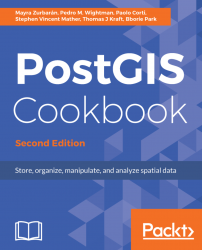
- Query PostGIS to get a list of the 100 active hotspots with the highest brightness temperature (the
bright_t31field) from theglobal_24htable created in the previous recipe:
      postgis_cookbook=# SELECTST_AsText(the_geom) AS the_geom, bright_t31
FROM chp01.global_24h
ORDER BY bright_t31 DESC LIMIT 100;
The output of the preceding command is as follows:
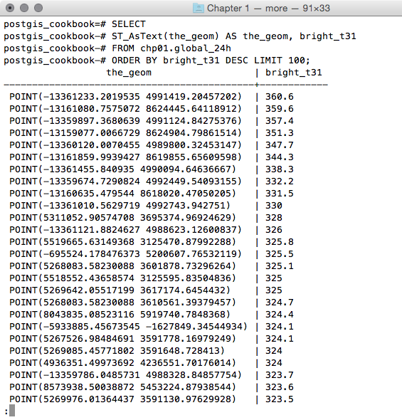
      postgis_cookbook=# SELECT ST_AsText(f.the_geom)
      AS the_geom, f.bright_t31, ac.iso2, ac.country_name
      FROM chp01.global_24h as f
      JOIN chp01.africa_countries as ac
      ON ST_Contains(ac.the_geom, ST_Transform(f.the_geom, 4326))
      ORDER BY f.bright_t31 DESCLIMIT 100;
The output of the preceding command is as follows:
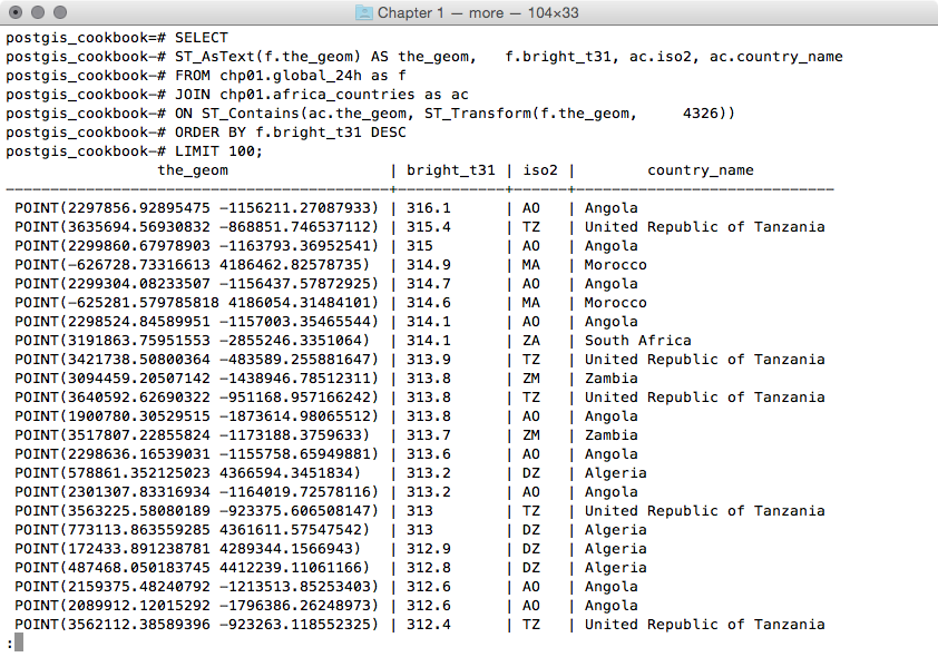
You will now export the result of this query to a vector format supported by GDAL, such as GeoJSON, in the WGS 84 spatial reference using ogr2ogr:
      $ ogr2ogr -f GeoJSON -t_srs EPSG:4326 warmest_hs.geojson
      PG:"dbname='postgis_cookbook' user='me' password='mypassword'" -sql "
      SELECT f.the_geom as the_geom, f.bright_t31,
             ac.iso2, ac.country_name
      FROM chp01.global_24h as f JOIN chp01.africa_countries as ac
      ON ST_Contains(ac.the_geom, ST_Transform(f.the_geom, 4326))
ORDER BY f.bright_t31 DESC LIMIT 100"- Open the GeoJSON file and inspect it with your favorite desktop GIS. The following screenshot shows you how it looks with QGIS:
      $ ogr2ogr -t_srs EPSG:4326 -f CSV -lco GEOMETRY=AS_XY
      -lco SEPARATOR=TAB warmest_hs.csv PG:"dbname='postgis_cookbook'
       user='me' password='mypassword'" -sql "
       SELECT f.the_geom, f.bright_t31,
         ac.iso2, ac.country_name
       FROM chp01.global_24h as f JOIN chp01.africa_countries as ac
       ON ST_Contains(ac.the_geom, ST_Transform(f.the_geom, 4326))
ORDER BY f.bright_t31 DESC LIMIT 100"GDAL is an open source library that comes together with several command-line utilities, which let the user translate and process raster and vector geodatasets into a plethora of formats. In the case of vector datasets, there is a GDAL sublibrary for managing vector datasets named OGR (therefore, when talking about vector datasets in the context of GDAL, we can also use the expression OGR dataset).
When you are working with an OGR dataset, two of the most popular OGR commands are ogrinfo, which lists many kinds of information from an OGR dataset, and ogr2ogr, which converts the OGR dataset from one format to another.
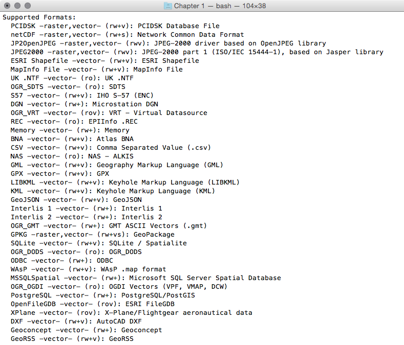
It is possible to retrieve a list of the supported OGR vector formats using the -formats option on any OGR commands, for example, with ogr2ogr:
$ ogr2ogr --formatsThe output of the preceding command is as follows:
Note that some formats are read-only, while others are read/write.
PostGIS is one of the supported read/write OGR formats, so it is possible to use the OGR API or any OGR commands (such as ogrinfo and ogr2ogr) to manipulate its datasets.
The ogr2ogr command has many options and parameters; in this recipe, you have seen some of the most notable ones such as -f to define the output format, -t_srs to reproject/transform the dataset, and -sql to define an (eventually spatial) query in the input OGR dataset.
When using ogrinfo and ogr2ogr together with the desired option and parameters, you have to define the datasets. When specifying a PostGIS dataset, you need a connection string that is defined as follows:
PG:"dbname='postgis_cookbook' user='me' password='mypassword'"You can find more information about the ogrinfo and ogr2ogr commands on the GDAL website available at http://www.gdal.org.
If you need more information about the PostGIS driver, you should check its related documentation page available at http://www.gdal.org/drv_pg.html.
In many GIS workflows, there is a typical scenario where subsets of a PostGIS table must be deployed to external users in a filesystem format (most typically, shapefiles or a spatialite database). Often, there is also the reverse process, where datasets received from different users have to be uploaded to the PostGIS database.
In this recipe, we will simulate both of these data flows. You will first create the data flow for processing the shapefiles out of PostGIS, and then the reverse data flow for uploading the shapefiles.
You will do it using the power of bash scripting and the ogr2ogr command.
If you didn't follow all the other recipes, be sure to import the hotspots (Global_24h.csv) and the countries dataset (countries.shp) in PostGIS. The following is how to do it with ogr2ogr (you should import both the datasets in their original SRID, 4326, to make spatial operations faster):
- Import in PostGIS the
Global_24h.csvfile, using theglobal_24.vrtvirtual driver you created in a previous recipe:
      $ ogr2ogr -f PostgreSQL PG:"dbname='postgis_cookbook'
      user='me' password='mypassword'" -lco SCHEMA=chp01 global_24h.vrt
-lco OVERWRITE=YES -lco GEOMETRY_NAME=the_geom -nln hotspots- Import the countries shapefile using
ogr2ogr:
      $ ogr2ogr -f PostgreSQL -sql "SELECT ISO2, NAME AS country_name
      FROM wborders" -nlt MULTIPOLYGON PG:"dbname='postgis_cookbook'
      user='me' password='mypassword'" -nln countries
      -lco SCHEMA=chp01 -lco OVERWRITE=YES
      -lco GEOMETRY_NAME=the_geom wborders.shp
Note
If you already imported the hotspots dataset using the 3857 SRID, you can use the PostGIS 2.0 method that allows the user to modify the geometry type column of an existing spatial table. You can update the SRID definition for the hotspots table in this way thanks to the support of typmod on geometry objects:postgis_cookbook=# ALTER TABLE chp01.hotspotsALTER COLUMN the_geomSET DATA TYPE geometry(Point, 4326)USING ST_Transform(the_geom, 4326);
The steps you need to follow to complete this recipe are as follows:
      postgis_cookbook=> SELECT c.country_name, MIN(c.iso2)
      as iso2, count(*) as hs_count FROM chp01.hotspots as hs
      JOIN chp01.countries as c ON ST_Contains(c.the_geom, hs.the_geom)
      GROUP BY c.country_name ORDER BY c.country_name;
The output of the preceding command is as follows:

- Using the same query, generate a CSV file using the PostgreSQL
COPYcommand or theogr2ogrcommand (in the first case, make sure that the Postgre service user has full write permission to the output directory). If you are following theCOPYapproach and using Windows, be sure to replace/tmp/hs_countries.csvwith a different path:
      $ ogr2ogr -f CSV hs_countries.csv
      PG:"dbname='postgis_cookbook' user='me' password='mypassword'"
      -lco SCHEMA=chp01 -sql "SELECT c.country_name, MIN(c.iso2) as iso2,
      count(*) as hs_count FROM chp01.hotspots as hs
      JOIN chp01.countries as c ON ST_Contains(c.the_geom, hs.the_geom)
      GROUP BY c.country_name ORDER BY c.country_name"
      postgis_cookbook=> COPY (SELECT c.country_name, MIN(c.iso2) as iso2,
      count(*) as hs_count  FROM chp01.hotspots as hs
      JOIN chp01.countries as c  ON ST_Contains(c.the_geom, hs.the_geom)
      GROUP BY c.country_name  ORDER BY c.country_name)
      TO '/tmp/hs_countries.csv' WITH CSV HEADER;
- If you are using Windows, go to step 5. With Linux, create a bash script named
export_shapefiles.shthat iterates each record (country) in thehs_countries.csvfile and generates a shapefile with the corresponding hotspots exported from PostGIS for that country:
        #!/bin/bash
        while IFS="," read country iso2 hs_count
        do
          echo "Generating shapefile $iso2.shp for country
          $country ($iso2) containing $hs_count features."
          ogr2ogr out_shapefiles/$iso2.shp
          PG:"dbname='postgis_cookbook' user='me' password='mypassword'"
          -lco SCHEMA=chp01 -sql "SELECT ST_Transform(hs.the_geom, 4326),
          hs.acq_date, hs.acq_time, hs.bright_t31
          FROM chp01.hotspots as hs JOIN chp01.countries as c
          ON ST_Contains(c.the_geom, ST_Transform(hs.the_geom, 4326))
WHERE c.iso2 = '$iso2'" done < hs_countries.csv - Give execution permissions to the
bashfile, and then run it after creating an output directory (out_shapefiles) for the shapefiles that will be generated by the script. Then, go to step 7:
      chmod 775 export_shapefiles.sh
      mkdir out_shapefiles
      $ ./export_shapefiles.sh
      Generating shapefile AL.shp for country
        Albania (AL) containing 66 features.
      Generating shapefile DZ.shp for country
        Algeria (DZ) containing 361 features.
...
      Generating shapefile ZM.shp for country
        Zambia (ZM) containing 1575 features.
      Generating shapefile ZW.shp for country
        Zimbabwe (ZW) containing 179 features.
Note
If you get the outputERROR: function getsrid(geometry) does not exist LINE 1: SELECT getsrid("the_geom") FROM (SELECT,..., you will need to load legacy support in PostGIS, for example, in a Debian Linux box:psql -d postgis_cookbook -f /usr/share/postgresql/9.1/contrib/postgis-2.1/legacy.sql
        @echo off
        for /f "tokens=1-3 delims=, skip=1" %%a in (hs_countries.csv) do (
          echo "Generating shapefile %%b.shp for country %%a
                (%%b) containing %%c features"
          ogr2ogr .\out_shapefiles\%%b.shp
          PG:"dbname='postgis_cookbook' user='me' password='mypassword'"
          -lco SCHEMA=chp01 -sql "SELECT ST_Transform(hs.the_geom, 4326),
          hs.acq_date, hs.acq_time, hs.bright_t31
          FROM chp01.hotspots as hs JOIN chp01.countries as c
          ON ST_Contains(c.the_geom, ST_Transform(hs.the_geom, 4326))
          WHERE c.iso2 = '%%b'"
) - Run the batch file after creating an output directory (
out_shapefiles) for the shapefiles that will be generated by the script:
      >mkdir out_shapefiles
      >export_shapefiles.bat
      "Generating shapefile AL.shp for country
       Albania (AL) containing 66 features"
      "Generating shapefile DZ.shp for country
       Algeria (DZ) containing 361 features"
      ...
      "Generating shapefile ZW.shp for country
       Zimbabwe (ZW) containing 179 features"
- Try to open a couple of these output shapefiles in your favorite desktop GIS. The following screenshot shows you how they look in QGIS:

- Now, you will do the return trip, uploading all of the generated shapefiles to PostGIS. You will upload all of the features for each shapefile and include the upload datetime and the original shapefile name. First, create the following PostgreSQL table, where you will upload the shapefiles:
      postgis_cookbook=# CREATE TABLE chp01.hs_uploaded
      (
        ogc_fid serial NOT NULL,
        acq_date character varying(80),
        acq_time character varying(80),
        bright_t31 character varying(80),
        iso2 character varying,
        upload_datetime character varying,
        shapefile character varying,
        the_geom geometry(POINT, 4326),
        CONSTRAINT hs_uploaded_pk PRIMARY KEY (ogc_fid)
      );
- If you are using Windows, go to step 12. With OS X, you will need to install
findutilswithhomebrewand run the script for Linux:
$ brew install findutils #!/bin/bash
for f in `find out_shapefiles -name \*.shp -printf "%f\n"`
do
echo "Importing shapefile $f to chp01.hs_uploaded PostGIS
table..." #, ${f%.*}"
ogr2ogr -append -update -f PostgreSQL
PG:"dbname='postgis_cookbook' user='me'
password='mypassword'" out_shapefiles/$f
-nln chp01.hs_uploaded -sql "SELECT acq_date, acq_time,
bright_t31, '${f%.*}' AS iso2, '`date`' AS upload_datetime,
'out_shapefiles/$f' as shapefile FROM ${f%.*}"
done - Assign the execution permission to the bash script and execute it:
      $ chmod 775 import_shapefiles.sh
      $ ./import_shapefiles.sh
      Importing shapefile DO.shp to chp01.hs_uploaded PostGIS table
      ...
      Importing shapefile ID.shp to chp01.hs_uploaded PostGIS table
      ...
      Importing shapefile AR.shp to chp01.hs_uploaded PostGIS table
      ......
Now, go to step 14.
- If you are using Windows, create a batch script named
import_shapefiles.bat:
        @echo off
        for %%I in (out_shapefiles\*.shp*) do (
          echo Importing shapefile %%~nxI to chp01.hs_uploaded
          PostGIS table...

          ogr2ogr -append -update  -f PostgreSQL
          PG:"dbname='postgis_cookbook' user='me'
          password='password'" out_shapefiles/%%~nxI
-nln chp01.hs_uploaded -sql "SELECT acq_date, acq_time,
bright_t31, '%%~nI' AS iso2, '%date%' AS upload_datetime,
'out_shapefiles/%%~nxI' as shapefile FROM %%~nI"
) - Run the batch script:
      >import_shapefiles.bat
      Importing shapefile AL.shp to chp01.hs_uploaded PostGIS table...
      Importing shapefile AO.shp to chp01.hs_uploaded PostGIS table...
      Importing shapefile AR.shp to chp01.hs_uploaded PostGIS table......
- Check some of the records that have been uploaded to the PostGIS table by using SQL:
      postgis_cookbook=# SELECT upload_datetime,
      shapefile, ST_AsText(wkb_geometry)
      FROM chp01.hs_uploaded WHERE ISO2='AT';
The output of the preceding command is as follows:

- Check the same query with
ogrinfoas well:
      $ ogrinfo PG:"dbname='postgis_cookbook' user='me'
      password='mypassword'"
      chp01.hs_uploaded -where "iso2='AT'"
The output of the preceding command is as follows:

You could implement both the data flows (processing shapefiles out from PostGIS, and then into it again) thanks to the power of the ogr2ogr GDAL command.
You have been using this command in different forms and with the most important input parameters in other recipes, so you should now have a good understanding of it.
Here, it is worth mentioning the way OGR lets you export the information related to the current datetime and the original shapefile name to the PostGIS table. Inside the import_shapefiles.sh (Linux, OS X) or the import_shapefiles.bat (Windows) scripts, the core is the line with the ogr2ogr command (here is the Linux version):
ogr2ogr -append -update -f PostgreSQL PG:"dbname='postgis_cookbook' user='me' password='mypassword'" out_shapefiles/$f -nln chp01.hs_uploaded -sql "SELECT acq_date, acq_time, bright_t31, '${f%.*}' AS iso2, '`date`' AS upload_datetime, 'out_shapefiles/$f' as shapefile FROM ${f%.*}"Thanks to the -sql option, you can specify the two additional fields, getting their values from the system date command and the filename that is being iterated from the script.
In this recipe, you will export a PostGIS table to a shapefile using the pgsql2shp command that is shipped with any PostGIS distribution.
The steps you need to follow to complete this recipe are as follows:
- In case you still haven't done it, export the countries shapefile to PostGIS using the
ogr2ogror theshp2pgsqlcommands. Theshp2pgsqlapproach is as shown:
      $ shp2pgsql -I -d -s 4326 -W LATIN1 -g the_geom countries.shp
      chp01.countries > countries.sql
      $ psql -U me -d postgis_cookbook -f countries.sql
- The
ogr2ograpproach is as follows:
      $ ogr2ogr -f PostgreSQL PG:"dbname='postgis_cookbook' user='me'
      password='mypassword'"
      -lco SCHEMA=chp01 countries.shp -nlt MULTIPOLYGON -lco OVERWRITE=YES
-lco GEOMETRY_NAME=the_geom- Now, query PostGIS in order to get a list of countries grouped by the
subregionfield. For this purpose, you will merge the geometries for features having the samesubregioncode, using theST_UnionPostGIS geometric processing function:
      postgis_cookbook=> SELECT subregion,
        ST_Union(the_geom) AS the_geom, SUM(pop2005) AS pop2005
FROM chp01.countries GROUP BY subregion;- Execute the
pgsql2shpPostGIS command to export into a shapefile the result of the given query:
      $ pgsql2shp -f subregions.shp -h localhost -u me -P mypassword
      postgis_cookbook "SELECT MIN(subregion) AS subregion,
      ST_Union(the_geom) AS the_geom, SUM(pop2005) AS pop2005
      FROM chp01.countries GROUP BY subregion;"

      Initializing...
      Done (postgis major version: 2).
      Output shape: Polygon
Dumping: X [23 rows].- Open the shapefile and inspect it with your favorite desktop GIS. This is how it looks in QGIS after applying a graduated classification symbology style based on the aggregated population for each subregion:

Visualization in QGIS of the classification of subregions based on population and information of the selected feature
You have exported the results of a spatial query to a shapefile using the pgsql2shp PostGIS command. The spatial query you have used aggregates fields using the SUM PostgreSQL function for summing country populations in the same subregion, and the ST_Union PostGIS function to aggregate the corresponding geometries as a geometric union.
The pgsql2shp command allows you to export PostGIS tables and queries to shapefiles. The options you need to specify are quite similar to the ones you use to connect to PostgreSQL with psql. To get a full list of these options, just type pgsql2shp in your command prompt and read the output.
In this recipe, you will import OpenStreetMap (OSM) data to PostGIS using the osm2pgsql command.
You will first download a sample dataset from the OSM website, and then you will import it using the osm2pgsql command.
You will add the imported layers in GIS desktop software and generate a view to get subdatasets, using the hstore PostgreSQL additional module to extract features based on their tags.
We need the following in place before we can proceed with the steps required for the recipe:
- Install
osm2pgsql. If you are using Windows, follow the instructions available at http://wiki.openstreetmap.org/wiki/Osm2pgsql. If you are on Linux, you can install it from the preceding website or from packages. For example, for Debian distributions, use the following:
$ sudo apt-get install osm2pgsql- For more information about the installation of the
osm2pgsqlcommand for other Linux distributions, macOS X, and MS Windows, please refer to theosm2pgsqlweb page available at http://wiki.openstreetmap.org/wiki/Osm2pgsql. - It's most likely that you will need to compile
osm2pgsqlyourself as the one that is installed with your package manager could already be obsolete. In my Linux Mint 12 box, this was the case (it wasosm2pgsqlv0.75), so I have installed Version 0.80 by following the instructions on theosm2pgsqlweb page. You can check the installed version just by typing the following command:
$ osm2pgsqlosm2pgsql SVN version 0.80.0 (32bit id space)
- We will create a different database only for this recipe, as we will use this OSM database in other chapters. For this purpose, create a new database named
romeand assign privileges to your user:
      postgres=# CREATE DATABASE rome OWNER me;
      postgres=# \connect rome;
      rome=# create extension postgis;
- You will not create a different schema in this new database, though, as the
osm2pgsqlcommand can only import OSM data in the public schema at the time of writing. - Be sure that your PostgreSQL installation supports
hstore(besidesPostGIS). If not, download and install it; for example, in Debian-based Linux distributions, you will need to install thepostgresql-contrib-9.6package. Then, addhstoresupport to theromedatabase using theCREATE EXTENSIONsyntax:
      $ sudo apt-get update
      $ sudo apt-get install postgresql-contrib-9.6
      $ psql -U me -d romerome=# CREATE EXTENSION hstore;
The steps you need to follow to complete this recipe are as follows:
- Download an
.osmfile from the OpenStreetMap website (https://www.openstreetmap.org/#map=5/21.843/82.795).
- Go to the OpenStreetMap website.
- Select the area of interest for which you want to export data. You should not select a large area, as the live export from the website is limited to 50,000 nodes.
Note
If you want to export larger areas, you should consider downloading the whole database, built daily at planet.osm (250 GB uncompressed and 16 GB compressed). At planet.osm, you may also download extracts that contain OpenstreetMap data for individual continents, countries, and metropolitan areas.
- If you want to get the same dataset used for this recipe, just copy and paste the following URL in your browser: http://www.openstreetmap.org/export?lat=41.88745&lon=12.4899&zoom=15&layers=M; or, get it from the book datasets (
chp01/map.osmfile). - Click on the
Exportlink. - Select
OpenStreetMap XML Dataas the output format. - Download the
map.osmfile to your working directory.
- If you want to get the same dataset used for this recipe, just copy and paste the following URL in your browser: http://www.openstreetmap.org/export?lat=41.88745&lon=12.4899&zoom=15&layers=M; or, get it from the book datasets (
- Run
osm2pgsqlto import the OSM data in the PostGIS database. Use the-hstoreoption, as you wish to add tags with an additionalhstore(key/value) column in the PostgreSQL tables:
      $ osm2pgsql -d rome -U me --hstore map.osm
      osm2pgsql SVN version 0.80.0 (32bit id space)Using projection
      SRS 900913 (Spherical Mercator)Setting up table:
      planet_osm_point...All indexes on planet_osm_polygon created
      in 1sCompleted planet_osm_polygonOsm2pgsql took 3s overall
- At this point, you should have the following geometry tables in your database:
      rome=# SELECT f_table_name, f_geometry_column,
      coord_dimension, srid, type FROM geometry_columns;
The output of the preceding command is shown here:
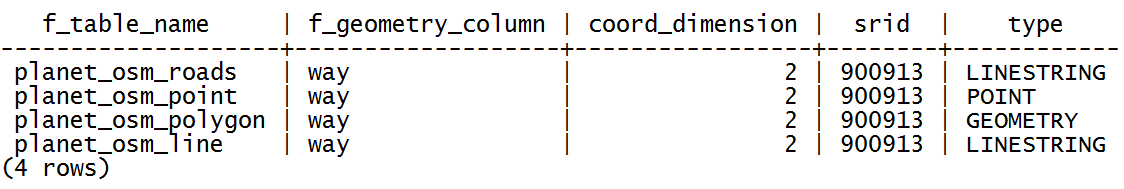
- Note that the
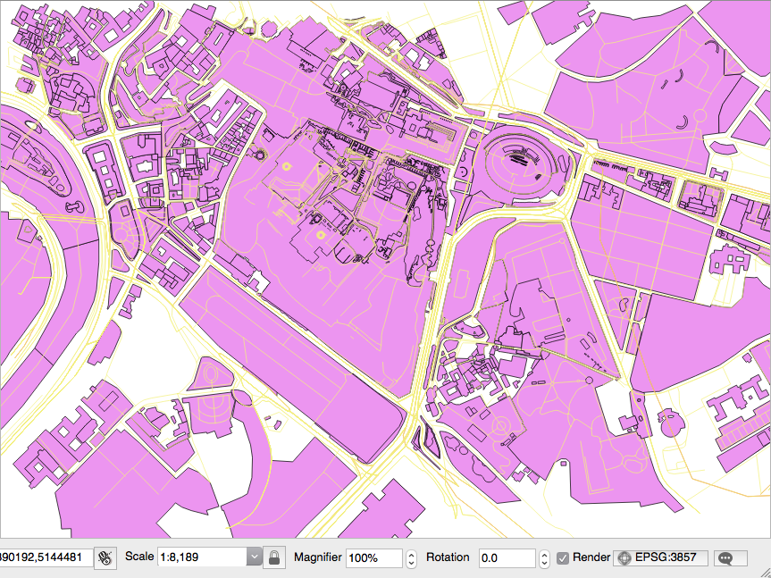
osm2pgsqlcommand imports everything in the public schema. If you did not deal differently with the command's input parameter, your data will be imported in the Mercator Projection (3857). - Open the PostGIS tables and inspect them with your favorite desktop GIS. The following screenshot shows how it looks in QGIS. All the different thematic features are mixed at this time, so it looks a bit confusing:
- Generate a PostGIS view that extracts all the polygons tagged with
treesasland cover. For this purpose, create the following view:
      rome=# CREATE VIEW rome_trees AS SELECT way, tags
      FROM planet_osm_polygon WHERE (tags -> 'landcover') = 'trees';
- Open the view with a desktop GIS that supports PostGIS views, such as QGIS, and add your
rome_treesview. The previous screenshot shows you how it looks.
OpenStreetMap is a popular collaborative project for creating a free map of the world. Every user participating in the project can edit data; at the same time, it is possible for everyone to download those datasets in .osm datafiles (an XML format) under the terms of the Open Data Commons Open Database License (ODbL) at the time of writing.
The osm2pgsql command is a command-line tool that can import .osm datafiles (eventually zipped) to the PostGIS database. To use the command, it is enough to give the PostgreSQL connection parameters and the .osm file to import.
It is possible to import only features that have certain tags in the spatial database, as defined in the default.style configuration file. You can decide to comment in or out the OSM tagged features that you would like to import, or not, from this file. The command by default exports all the nodes and ways to linestring, point, and geometry PostGIS geometries.
It is highly recommended to enable hstore support in the PostgreSQL database and use the -hstore option of osm2pgsql when importing the data. Having enabled this support, the OSM tags for each feature will be stored in a hstore PostgreSQL data type, which is optimized for storing (and retrieving) sets of key/values pairs in a single field. This way, it will be possible to query the database as follows:
SELECT way, tags FROM planet_osm_polygon WHERE (tags -> 'landcover') = 'trees';PostGIS 2.0 now has full support for raster datasets, and it is possible to import raster datasets using the raster2pgsql command.
In this recipe, you will import a raster file to PostGIS using the raster2pgsql command. This command, included in any PostGIS distribution from version 2.0 onward, is able to generate an SQL dump to be loaded in PostGIS for any GDAL raster-supported format (in the same fashion that the shp2pgsql command does for shapefiles).
After loading the raster to PostGIS, you will inspect it both with SQL commands (analyzing the raster metadata information contained in the database), and with the gdalinfo command-line utility (to understand the way the input raster2pgsql parameters have been reflected in the PostGIS import process).
You will finally open the raster in a desktop GIS and try a basic spatial query, mixing vector and raster tables.
We need the following in place before we can proceed with the steps required for the recipe:
- From the worldclim website, download the current raster data (http://www.worldclim.org/current) for min and max temperatures (only the raster for max temperatures will be used for this recipe). Alternatively, use the ones provided in the book datasets (
data/chp01). Each of the two archives (data/tmax_10m_bil.zipanddata/tmin_10m_bil.zip) contain 12 rasters in the BIL format, one for each month. You can look for more information at http://www.worldclim.org/formats. - Extract the two archives to a directory named
worldclimin your working directory. - Rename each raster dataset to a name format with two digits for the month, for example,
tmax1.bilandtmax1.hdrwill becometmax01.bilandtmax01.hdr. - If you still haven't loaded the countries shapefile to PostGIS from a previous recipe, do it using the
ogr2ogrorshp2pgsqlcommands. The following is theshp2pgsqlsyntax:
      $ shp2pgsql -I -d -s 4326 -W LATIN1 -g the_geom countries.shp
      chp01.countries > countries.sql
      $ psql -U me -d postgis_cookbook -f countries.sql
The steps you need to follow to complete this recipe are as follows:
- Get information about one of the rasters using the
gdalinfocommand-line tool as follows:
      $ gdalinfo worldclim/tmax09.bil

      Driver: EHdr/ESRI .hdr Labelled
      Files: worldclim/tmax9.bil
worldclim/tmax9.hdr
      Size is 2160, 900
      Coordinate System is:
      GEOGCS[""WGS 84"",
        DATUM[""WGS_1984"",
          SPHEROID[""WGS 84"",6378137,298.257223563,
            AUTHORITY[""EPSG"",""7030""]],
          TOWGS84[0,0,0,0,0,0,0],
          AUTHORITY[""EPSG"",""6326""]],
        PRIMEM[""Greenwich"",0,
          AUTHORITY[""EPSG"",""8901""]],
        UNIT[""degree"",0.0174532925199433,
        AUTHORITY[""EPSG"",""9108""]],
      AUTHORITY[""EPSG"",""4326""]]
      Origin = (-180.000000000000057,90.000000000000000)
      Pixel Size = (0.166666666666667,-0.166666666666667)
      Corner Coordinates:
Upper Left (-180.0000000, 90.0000000) (180d 0'' 0.00""W, 90d
                                               0'' 0.00""N)
Lower Left (-180.0000000, -60.0000000) (180d 0'' 0.00""W, 60d
                                                0'' 0.00""S)
Upper Right ( 180.0000000, 90.0000000) (180d 0'' 0.00""E, 90d
                                                0'' 0.00""N)
Lower Right ( 180.0000000, -60.0000000) (180d 0'' 0.00""E, 60d
                                                 0'' 0.00""S)
Center ( 0.0000000, 15.0000000) ( 0d 0'' 0.00""E, 15d
                                          0'' 0.00""N)
        Band 1 Block=2160x1 Type=Int16, ColorInterp=Undefined
        Min=-153.000 Max=441.000
        NoData Value=-9999
- The
gdalinfocommand provides a lot of useful information about the raster, for example, the GDAL driver being used to read it, the files composing it (in this case, two files with.biland.hdrextensions), the size in pixels (2160 x 900), the spatial reference (WGS 84), the geographic extents, the origin, and the pixel size (needed to correctly georeference the raster), and for each raster band (just one in the case of this file), some statistical information like the min and max values (-153.000 and 441.000, corresponding to a temperature of -15.3 °C and 44.1 °C. Values are expressed as temperature * 10 in °C, according to the documentation available at http://worldclim.org/). - Use the
raster2pgsqlfile to generate the.sqldump file and then import the raster in PostGIS:
      $ raster2pgsql -I -C -F -t 100x100 -s 4326
      worldclim/tmax01.bil chp01.tmax01 > tmax01.sql
      $ psql -d postgis_cookbook -U me -f tmax01.sql
If you are in Linux, you may pipe the two commands in a unique line:
      $ raster2pgsql -I -C -M -F -t 100x100 worldclim/tmax01.bil
chp01.tmax01 | psql -d postgis_cookbook -U me -f tmax01.sql- Check how the new table has been created in PostGIS:
      $ pg_dump -t chp01.tmax01 --schema-only -U me postgis_cookbook
      ...
      CREATE TABLE tmax01 (
        rid integer NOT NULL,
        rast public.raster,
        filename text,
        CONSTRAINT enforce_height_rast CHECK (
          (public.st_height(rast) = 100)
        ),
        CONSTRAINT enforce_max_extent_rast CHECK (public.st_coveredby
          (public.st_convexhull(rast), ''0103...''::public.geometry)
        ),
        CONSTRAINT enforce_nodata_values_rast CHECK (
          ((public._raster_constraint_nodata_values(rast)
            )::numeric(16,10)[] = ''{0}''::numeric(16,10)[])
          ),
        CONSTRAINT enforce_num_bands_rast CHECK (
          (public.st_numbands(rast) = 1)
        ),
        CONSTRAINT enforce_out_db_rast CHECK (
          (public._raster_constraint_out_db(rast) = ''{f}''::boolean[])
          ),
        CONSTRAINT enforce_pixel_types_rast CHECK (
          (public._raster_constraint_pixel_types(rast) =
           ''{16BUI}''::text[])
          ),
        CONSTRAINT enforce_same_alignment_rast CHECK (
          (public.st_samealignment(rast, ''01000...''::public.raster)
        ),
        CONSTRAINT enforce_scalex_rast CHECK (
          ((public.st_scalex(rast))::numeric(16,10) =
            0.166666666666667::numeric(16,10))
           ),
        CONSTRAINT enforce_scaley_rast CHECK (
          ((public.st_scaley(rast))::numeric(16,10) =
            (-0.166666666666667)::numeric(16,10))
          ),
        CONSTRAINT enforce_srid_rast CHECK ((public.st_srid(rast) = 0)),
        CONSTRAINT enforce_width_rast CHECK ((public.st_width(rast) = 100))
);- Check if a record for this PostGIS raster appears in the
raster_columnsmetadata view, and note the main metadata information that has been stored there, such as schema, name, raster column name (default is raster), SRID, scale (for x and y), block size (for x and y), band numbers (1), band types (16BUI), zero data values (0), anddbstorage type (out_dbisfalse, as we have stored the raster bytes in the database; you could have used the-Roption to register the raster as an out-of-db filesystem):
postgis_cookbook=# SELECT * FROM raster_columns;
- If you have followed this recipe from the beginning, you should now have 198 rows in the raster table, with each row representing one raster block size (100 x 100 pixels blocks, as indicated with the
-traster2pgsqloption):
postgis_cookbook=# SELECT count(*) FROM chp01.tmax01;The output of the preceding command is as follows:
      count
      -------
      198
      (1 row)
- Try to open the raster table with
gdalinfo. You should see the same information you got fromgdalinfowhen you were analyzing the original BIL file. The only difference is the block size, as you moved to a smaller one (100 x 100) from the original (2160 x 900). That's why the original file has been split into several datasets (198):
      gdalinfo PG":host=localhost port=5432 dbname=postgis_cookbook
user=me password=mypassword schema='chp01' table='tmax01'"- The
gdalinfocommand reads the PostGIS raster as being composed of multiple raster subdatasets (198, one for each row in the table). You still have the possibility of reading the whole table as a single raster, using themode=2option in the PostGIS raster connection string (mode=1is the default). Check the difference:
      gdalinfo PG":host=localhost port=5432 dbname=postgis_cookbook
user=me password=mypassword schema='chp01' table='tmax01' mode=2"- You can easily obtain a visual representation of those blocks by converting the extent of all the 198 rows in the
tmax01table (each representing a raster block) to a shapefile usingogr2ogr:
      $ ogr2ogr temp_grid.shp PG:"host=localhost port=5432
      dbname='postgis_cookbook' user='me' password='mypassword'"
      -sql "SELECT rid, filename, ST_Envelope(rast) as the_geom
FROM chp01.tmax01"- Now, try to open the raster table with QGIS (at the time of writing, one of the few desktop GIS tools that has support for it) together with the blocks shapefile generated in the previous steps (
temp_grid.shp). You should see something like the following screenshot:

Note
If you are using QGIS 2.6 or higher, you can see the layer in the DB Manager under the Database menu and drag it to the Layers panel.
- As the last bonus step, you will select the 10 countries with the lowest average max temperature in January (using the centroid of the polygon representing the country):
      SELECT * FROM (
        SELECT c.name, ST_Value(t.rast,
          ST_Centroid(c.the_geom))/10 as tmax_jan FROM chp01.tmax01 AS t
        JOIN chp01.countries AS c
        ON ST_Intersects(t.rast, ST_Centroid(c.the_geom))
      ) AS foo
      ORDER BY tmax_jan LIMIT 10;
The output is as follows:

The raster2pgsql command is able to load any raster formats supported by GDAL in PostGIS. You can have a format list supported by your GDAL installation by typing the following command:
$ gdalinfo --formatsIn this recipe, you have been importing one raster file using some of the most common raster2pgsql options:
$ raster2pgsql -I -C -F -t 100x100 -s 4326 worldclim/tmax01.bil chp01.tmax01 > tmax01.sqlThe -I option creates a GIST spatial index for the raster column. The -C option will create the standard set of constraints after the rasters have been loaded. The -F option will add a column with the filename of the raster that has been loaded. This is useful when you are appending many raster files to the same PostGIS raster table. The -s option sets the raster's SRID.
If you decide to include the -t option, then you will cut the original raster into tiles, each inserted as a single row in the raster table. In this case, you decided to cut the raster into 100 x 100 tiles, resulting in 198 table rows in the raster table.
Another important option is -R, which will register the raster as out-of-db; in such a case, only the metadata will be inserted in the database, while the raster will be out of the database.
The raster table contains an identifier for each row, the raster itself (eventually one of its tiles, if using the -t option), and eventually the original filename, if you used the -F option, as in this case.
You can analyze the PostGIS raster using SQL commands or the gdalinfo command. Using SQL, you can query the raster_columns view to get the most significant raster metadata (spatial reference, band number, scale, block size, and so on).
With gdalinfo, you can access the same information, using a connection string with the following syntax:
gdalinfo PG":host=localhost port=5432 dbname=postgis_cookbook user=me password=mypassword schema='chp01' table='tmax01' mode=2"The mode parameter is not influential if you loaded the whole raster as a single block (for example, if you did not specify the -t option). But, as in the use case of this recipe, if you split it into tiles, gdalinfo will see each tile as a single subdataset with the default behavior (mode=1). If you want GDAL to consider the raster table as a unique raster dataset, you have to specify the mode option and explicitly set it to 2.
This recipe will guide you through the importing of multiple rasters at a time.
You will first import some different single band rasters to a unique single band raster table using the raster2pgsql command.
Then, you will try an alternative approach, merging the original single band rasters in a virtual raster, with one band for each of the original rasters, and then load the multiband raster to a raster table. To accomplish this, you will use the GDAL gdalbuildvrt command and then load the data to PostGIS with raster2pgsql.
Be sure to have all the original raster datasets you have been using for the previous recipe.
The steps you need to follow to complete this recipe are as follows:
- Import all the maximum average temperature rasters in a single PostGIS raster table using
raster2pgsqland thenpsql(eventually, pipe the two commands if you are in Linux):
      $ raster2pgsql -d -I -C -M -F -t 100x100 -s 4326
      worldclim/tmax*.bil chp01.tmax_2012 > tmax_2012.sql
      $ psql -d postgis_cookbook -U me -f tmax_2012.sql
- Check how the table was created in PostGIS, querying the
raster_columnstable. Here we are querying only some significant fields:
      postgis_cookbook=# SELECT r_raster_column, srid,
      ROUND(scale_x::numeric, 2) AS scale_x,
      ROUND(scale_y::numeric, 2) AS scale_y, blocksize_x,
      blocksize_y, num_bands, pixel_types, nodata_values, out_db
      FROM raster_columns where r_table_schema='chp01'
      AND r_table_name ='tmax_2012';
      SELECT rid, (foo.md).*
      FROM (SELECT rid, ST_MetaData(rast) As md
FROM chp01.tmax_2012) As foo;The output of the preceding command is as shown here:

If you now query the table, you would be able to derive the month for each raster row only from the
original_filecolumn. In the table, you have imported 198 distinct records (rasters) for each of the 12 original files (we divided them into 100 x 100 blocks, if you remember). Test this with the following query:
      postgis_cookbook=# SELECT COUNT(*) AS num_raster,
      MIN(filename) as original_file FROM chp01.tmax_2012
GROUP BY filename ORDER BY filename;

- With this approach, using the
filenamefield, you could use theST_ValuePostGIS raster function to get the average monthly maximum temperature of a certain geographic zone for the whole year:
      SELECT REPLACE(REPLACE(filename, 'tmax', ''), '.bil', '') AS month,
      (ST_VALUE(rast, ST_SetSRID(ST_Point(12.49, 41.88), 4326))/10) AS tmax
      FROM chp01.tmax_2012
      WHERE rid IN (
        SELECT rid FROM chp01.tmax_2012
        WHERE ST_Intersects(ST_Envelope(rast),
              ST_SetSRID(ST_Point(12.49, 41.88), 4326))
      )
      ORDER BY month;
The output of the preceding command is as shown here:

- A different approach is to store each month value in a different raster band. The
raster2pgsqlcommand doesn't let you load to different bands in an existing table. But, you can use GDAL by combining thegdalbuildvrtand thegdal_translatecommands. First, usegdalbuildvrtto create a new virtual raster composed of 12 bands, one for each month:
$ gdalbuildvrt -separate tmax_2012.vrt worldclim/tmax*.bil- Analyze the
tmax_2012.vrtXML file with a text editor. It should have a virtual band (VRTRasterBand) for each physical raster pointing to it:
      <VRTDataset rasterXSize="2160" rasterYSize="900">
        <SRS>GEOGCS...</SRS>
        <GeoTransform>
          -1.8000000000000006e+02, 1.6666666666666699e-01, ...
        </GeoTransform>
        <VRTRasterBand dataType="Int16" band="1">
          <NoDataValue>-9.99900000000000E+03</NoDataValue>
          <ComplexSource>
            <SourceFilename relativeToVRT="1">
              worldclim/tmax01.bil
            </SourceFilename>
            <SourceBand>1</SourceBand>
            <SourceProperties RasterXSize="2160" RasterYSize="900"
             DataType="Int16" BlockXSize="2160" BlockYSize="1" />
            <SrcRect xOff="0" yOff="0" xSize="2160" ySize="900" />
            <DstRect xOff="0" yOff="0" xSize="2160" ySize="900" />
            <NODATA>-9999</NODATA>
          </ComplexSource>
        </VRTRasterBand>
      <VRTRasterBand dataType="Int16" band="2">
...- Now, with
gdalinfo, analyze this output virtual raster to check if it is effectively composed of 12 bands:
$ gdalinfo tmax_2012.vrtThe output of the preceding command is as follows:

- Import the virtual raster composed of 12 bands, each referring to one of the 12 original rasters, to a PostGIS raster table composed of 12 bands. For this purpose, you can use the
raster2pgsqlcommand:
      $ raster2pgsql -d -I -C -M -F -t 100x100 -s 4326 tmax_2012.vrt
      chp01.tmax_2012_multi > tmax_2012_multi.sql
      $ psql -d postgis_cookbook -U me -f tmax_2012_multi.sql
- Query the
raster_columnsview to get some indicators for the imported raster. Note that thenum_bandsis now 12:
     postgis_cookbook=# SELECT r_raster_column, srid, blocksize_x,
     blocksize_y, num_bands, pixel_types
     from raster_columns where r_table_schema='chp01'
     AND r_table_name ='tmax_2012_multi';
- Now, let's try to produce the same output as the query using the previous approach. This time, given the table structure, we keep the results in a single row:
      postgis_cookbook=# SELECT
      (ST_VALUE(rast, 1, ST_SetSRID(ST_Point(12.49, 41.88), 4326))/10)
      AS jan,
      (ST_VALUE(rast, 2, ST_SetSRID(ST_Point(12.49, 41.88), 4326))/10)
      AS feb,
      (ST_VALUE(rast, 3, ST_SetSRID(ST_Point(12.49, 41.88), 4326))/10)
      AS mar,
      (ST_VALUE(rast, 4, ST_SetSRID(ST_Point(12.49, 41.88), 4326))/10)
      AS apr,
      (ST_VALUE(rast, 5, ST_SetSRID(ST_Point(12.49, 41.88), 4326))/10)
      AS may,
      (ST_VALUE(rast, 6, ST_SetSRID(ST_Point(12.49, 41.88), 4326))/10)
      AS jun,
      (ST_VALUE(rast, 7, ST_SetSRID(ST_Point(12.49, 41.88), 4326))/10)
      AS jul,
      (ST_VALUE(rast, 8, ST_SetSRID(ST_Point(12.49, 41.88), 4326))/10)
      AS aug,
      (ST_VALUE(rast, 9, ST_SetSRID(ST_Point(12.49, 41.88), 4326))/10)
      AS sep,
      (ST_VALUE(rast, 10, ST_SetSRID(ST_Point(12.49, 41.88), 4326))/10)
      AS oct,
      (ST_VALUE(rast, 11, ST_SetSRID(ST_Point(12.49, 41.88), 4326))/10)
      AS nov,
      (ST_VALUE(rast, 12, ST_SetSRID(ST_Point(12.49, 41.88), 4326))/10)
      AS dec
      FROM chp01.tmax_2012_multi WHERE rid IN (
        SELECT rid FROM chp01.tmax_2012_multi
        WHERE ST_Intersects(rast, ST_SetSRID(ST_Point(12.49, 41.88), 4326))
      );
The output of the preceding command is as follows:

You can import raster datasets in PostGIS using the raster2pgsql command.
Note
The GDAL PostGIS raster so far does not support writing operations; therefore, for now, you cannot use GDAL commands such as gdal_translate and gdalwarp.
This is going to change in the near future, so you may have such an extra option when you are reading this chapter.
In a scenario where you have multiple rasters representing the same variable at different times, as in this recipe, it makes sense to store all of the original rasters as a single table in PostGIS. In this recipe, we have the same variable (average maximum temperature) represented by a single raster for each month. You have seen that you could proceed in two different ways:
- Append each single raster (representing a different month) to the same PostGIS single band raster table and derive the information related to the month from the value in the filename column (added to the table using the
-F raster2pgsqloption). - Generate a multiband raster using
gdalbuildvrt(one raster with 12 bands, one for each month), and import it in a single multiband PostGIS table using theraster2pgsqlcommand.
In this recipe, you will see a couple of main options for exporting PostGIS rasters to different raster formats. They are both provided as command-line tools, gdal_translate and gdalwarp, by GDAL.
You need the following in place before you can proceed with the steps required for the recipe:
- You need to have gone through the previous recipe and imported
tmax2012 datasets (12.bilfiles) as a single multiband (12 bands) raster in PostGIS. - You must have the PostGIS raster format enabled in GDAL. For this purpose, check the output of the following command:
$ gdalinfo --formats | grep -i postgisThe output of the preceding command is as follows:
PostGISRaster (rw): PostGIS Raster driver- You should have already learned how to use the GDAL PostGIS raster driver in the previous two recipes. You need to use a connection string composed of the following parameters:
      $ gdalinfo PG:"host=localhost port=5432
      dbname='postgis_cookbook' user='me' password='mypassword'
schema='chp01' table='tmax_2012_multi' mode='2'"- Refer to the previous two recipes for more information about the preceding parameters.
The steps you need to follow to complete this recipe are as follows:
- As an initial test, you will export the first six months of the
tmaxfor 2012 (the first six bands in thetmax_2012_multiPostGIS raster table) using thegdal_translatecommand:
      $ gdal_translate -b 1 -b 2 -b 3 -b 4 -b 5 -b 6
      PG:"host=localhost port=5432 dbname='postgis_cookbook'
      user='me' password='mypassword' schema='chp01'
table='tmax_2012_multi' mode='2'" tmax_2012_multi_123456.tif- As the second test, you will export all of the bands, but only for the geographic area containing Italy. Use the
ST_Extentcommand to get the geographic extent of that zone:
      postgis_cookbook=# SELECT ST_Extent(the_geom)
      FROM chp01.countries WHERE name = 'Italy';
The output of the preceding command is as follows:

- Now use the
gdal_translatecommand with the-projwinoption to obtain the desired purpose:
      $ gdal_translate -projwin 6.619 47.095 18.515 36.649
      PG:"host=localhost port=5432 dbname='postgis_cookbook'
      user='me' password='mypassword' schema='chp01'
table='tmax_2012_multi' mode='2'" tmax_2012_multi.tif- There is another GDAL command,
gdalwarp, that is still a convert utility with reprojection and advanced warping functionalities. You can use it, for example, to export a PostGIS raster table, reprojecting it to a different spatial reference system. This will convert the PostGIS raster table to GeoTiff and reproject it fromEPSG:4326toEPSG:3857:
      gdalwarp -t_srs EPSG:3857 PG:"host=localhost port=5432
      dbname='postgis_cookbook' user='me' password='mypassword'
      schema='chp01' table='tmax_2012_multi' mode='2'"
tmax_2012_multi_3857.tifBoth gdal_translate and gdalwarp can transform rasters from a PostGIS raster to all GDAL-supported formats. To get a complete list of the supported formats, you can use the --formats option of GDAL's command line as follows:
$ gdalinfo --formatsFor both these GDAL commands, the default output format is GeoTiff; if you need a different format, you must use the -of option and assign to it one of the outputs produced by the previous command line.
In this recipe, you have tried some of the most common options for these two commands. As they are complex tools, you may try some more command options as a bonus step.
To get a better understanding, you should check out the excellent documentation on the GDAL website:
- Information about the
gdal_translatecommand is available at http://www.gdal.org/gdal_translate.html - Information about the
gdalwarpcommand is available at http://www.gdal.org/gdalwarp.html