


Let's get started. We will install NumPy and related software on different operating systems and have a look at some simple code that uses NumPy. This chapter briefly introduces the IPython interactive shell. SciPy is closely related to NumPy, so you will see the SciPy name appearing here and there. At the end of this chapter, you will find pointers on how to find additional information online if you get stuck or are uncertain about the best way to solve problems.
In this chapter, you will cover the following topics:
Install Python, SciPy, matplotlib, IPython, and NumPy on Windows, Linux, and Macintosh
Do a short refresher of Python
Write simple NumPy code
Get to know IPython
Browse online documentation and resources
NumPy is based on Python, so you need to have Python installed. On some operating systems, Python is already installed. However, you need to check whether the Python version corresponds with the NumPy version you want to install. There are many implementations of Python, including commercial implementations and distributions. In this book, we focus on the standard CPython implementation, which is guaranteed to be compatible with NumPy.
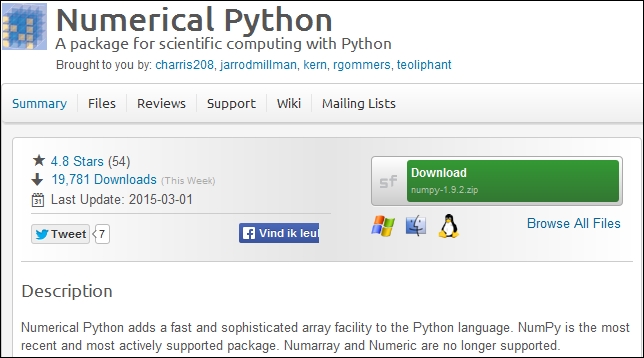
NumPy has binary installers for Windows, various Linux distributions, and Mac OS X at http://sourceforge.net/projects/numpy/files/. There is also a source distribution, if you prefer that. You need to have Python 2.4.x or above installed on your system. We will go through the various steps required to install Python on the following operating systems:
Debian and Ubuntu: Python might already be installed on Debian and Ubuntu, but the development headers are usually not. On Debian and Ubuntu, install the
pythonandpython-devpackages with the following commands:$ [sudo] apt-get install python $ [sudo] apt-get install python-dev
Windows: The Windows Python installer is available at https://www.python.org/downloads/. On this website, we can also find installers for Mac OS X and source archives for Linux, UNIX, and Mac OS X.
Mac: Python comes preinstalled on Mac OS X. We can also get Python through MacPorts, Fink, Homebrew, or similar projects.
Install, for instance, the Python 2.7 port by running the following command:
$ [sudo] port install python27Linear Algebra PACKage (LAPACK) does not need to be present but, if it is, NumPy will detect it and use it during the installation phase. It is recommended that you install LAPACK for serious numerical analysis as it has useful numerical linear algebra functionality.
We installed Python on Debian, Ubuntu, Windows, and the Mac OS X.
Note
You can download the example code files for all the Packt books you have purchased from your account at https://www.packtpub.com/. If you purchased this book elsewhere, you can visit https://www.packtpub.com/books/content/support and register to have the files e-mailed directly to you.
Before we start the NumPy introduction, let's take a brief tour of the Python help system, in case you have forgotten how it works or are not very familiar with it. The Python help system allows you to look up documentation from the interactive Python shell. A shell is an interactive program, which accepts commands and executes them for you.
Depending on your operating system, you can access the Python shell with special applications, usually a terminal of some sort.
In such a terminal, type the following command to start a Python shell:
$ pythonYou will get a short message with the Python version and other information and the following prompt:
>>>Type the following in the prompt:
>>> help()Another message appears and the prompt changes as follows:
help>If you type, for instance,
keywordsas the message says, you get a list of keywords. Thetopicscommand gives a list of topics. If you type any of the topic names (such as LISTS) in the prompt, you get additional information about the topic. Typingqquits the information screen. Pressing Ctrl + D together returns you to the normal Python prompt:>>>Pressing Ctrl + D together again ends the Python shell session.
In the Time for action – using the Python help system section, we used the Python shell to look up documentation. We can also use Python as a calculator. By the way, this is just a refresher, so if you are completely new to Python, I recommend taking some time to learn the basics. If you put your mind to it, learning basic Python should not take you more than a couple of weeks.
We can use Python as a calculator as follows:
In a Python shell, add 2 and 2 as follows:
>>> 2 + 2
4
Multiply 2 and 2 as follows:
>>> 2 * 2
4
Divide 2 and 2 as follows:
>>> 2/2
1
If you have programmed before, you probably know that dividing is a bit tricky since there are different types of dividing. For a calculator, the result is usually adequate, but the following division may not be what you were expecting:
>>> 3/2
1
We will discuss what this result is about in several later chapters of this book. Take the cube of 2 as follows:
>>> 2 ** 3
8
Assigning values to variables in Python works in a similar way to most programming languages.
For instance, assign the value of
2to a variable namedvaras follows:>>> var = 2 >>> var 2
We defined the variable and assigned it a value. In this Python code, the type of the variable is not fixed. We can make the variable in to a list, which is a built-in Python type corresponding to an ordered sequence of values. Assign a list to
varas follows:>>> var = [2, 'spam', 'eggs'] >>> var [2, 'spam', 'eggs']
We can assign a new value to a list item using its index number (counting starts from 0). Assign a new value to the first list element:
>>> var
['ham', 'spam', 'eggs']
We can also swap values easily. Define two variables and swap their values:
>>> a = 1
>>> b = 2
>>> a, b = b, a
>>> a
2
>>> b
1
We assigned values to variables and Python list items. This section is by no means exhaustive; therefore, if you are struggling, please read Appendix B, Additional Online Resources, to find recommended Python tutorials.
If you haven't programmed in Python for a while or are a Python novice, you may be confused about the Python 2 versus Python 3 discussions. In a nutshell, the latest version Python 3 is not backward compatible with the older Python 2 because the Python development team felt that some issues were fundamental and therefore warranted a radical change. The Python team has committed to maintain Python 2 until 2020. This may be problematic for the people who still depend on Python 2 in some way. The consequence for the print() function is that we have two types of syntax.
We can print using the print() function as follows:
The old syntax is as follows:
>>> print 'Hello'
Hello
The new Python 3 syntax is as follows:
>>> print('Hello')
Hello
The parentheses are now mandatory in Python 3. In this book, I try to use the new syntax as much as possible; however, I use Python 2 to be on the safe side. To enforce the syntax, each Python 2 script with
print()calls in this book starts with:>>> from __future__ import print_functionTry to use the old syntax to get the following error message:
>>> print 'Hello'
  File "<stdin>", line 1
    print 'Hello'
                ^
SyntaxError: invalid syntax
To print a newline, use the following syntax:
>>> print()To print multiple items, separate them with commas:
>>> print(2, 'ham', 'egg')
2 ham egg
By default, Python separates the printed values with spaces and prints output to the screen. You can customize these settings. Read more about this function by typing the following command:
>>> help(print)You can exit again by typing
q.
Commenting code is a best practice with the goal of making code clearer for yourself and other coders (see https://google-styleguide.googlecode.com/svn/trunk/pyguide.html?showone=Comments#Comments). Usually, companies and other organizations have policies regarding code comment such as comment templates. In this book, I did not comment the code in such a fashion for brevity and because the text in the book should clarify the code.
The most basic comment starts with a hash sign and continues until the end of the line:
Comment code with this type of comment as follows:
>>> # Comment from hash to end of lineHowever, if the hash sign is between single or double quotes, then we have a string, which is an ordered sequence of characters:
>>> astring = '# This is not a comment'
>>> astring
'# This is not a comment'
We can also comment multiple lines as a block. This is useful if you want to write a more detailed description of the code. Comment multiple lines as follows:
"""
 Chapter 1 of NumPy Beginners Guide.
 Another line of comment.
"""
We refer to this type of comment as triple-quoted for obvious reasons. It also is used to test code. You can read about testing in Chapter 8, Assuring Quality with Testing.
We can use the if statement in the following ways:
Check whether a number is negative as follows:
>>> if 42 < 0:
...     print('Negative')
... else:
...     print('Not negative')
...
Not negative
In the preceding example, Python decided that
42is not negative. Theelseclause is optional. The comparison operators are equivalent to the ones in C++, Java, and similar languages.Python also has a chained branching logic compound statement for multiple tests similar to the switch statement in C++, Java, and other programming languages. Decide whether a number is negative, 0, or positive as follows:
>>> a = -42
>>> if a < 0:
...     print('Negative')
... elif a == 0:
...     print('Zero')
... else:
...     print('Positive')
...
Negative
This time, Python decided that
42is negative.
We can use the for loop in the following ways:
Loop over an ordered sequence, such as a list, and print each item as follows:
>>> food = ['ham', 'egg', 'spam']
>>> for snack in food:
...     print(snack)
...
ham
egg
spam
And remember that, as always, indentation matters in Python. We loop over a range of values with the built-in
range()orxrange()functions. The latter function is slightly more efficient in certain cases. Loop over the numbers1-9with a step of 2 as follows:>>> for i in range(1, 9, 2): ... print(i) ... 1 3 5 7
The start and step parameter of the
range()function are optional with default values of1. We can also prematurely end a loop. Loop over the numbers0-9and break out of the loop when you reach3:>>> for i in range(9): ... print(i) ... if i == 3: ... print('Three') ... break ... 0 1 2 3 Three
The loop stopped at
3and we did not print the higher numbers. Instead of leaving the loop, we can also get out of the current iteration. Print the numbers0-4, skipping3as follows:>>> for i in range(5): ... if i == 3: ... print('Three') ... continue ... print(i) ... 0 1 2 Three 4
The last line in the loop was not executed when we reached
3because of thecontinuestatement. In Python, theforloop can have anelsestatement attached to it. Add anelseclause as follows:>>> for i in range(5): ... print(i) ... else: ... print(i, 'in else clause') ... 0 1 2 3 4 (4, 'in else clause')
Python executes the code in the
elseclause last. Python also has awhileloop. I do not use it that much because theforloop is more useful in my opinion.
Let's define the following simple function:
Print
Helloand a given name in the following way:>>> def print_hello(name): ... print('Hello ' + name) ...
Call the function as follows:
>>> print_hello('Ivan')
Hello Ivan
Some functions do not have arguments, or the arguments have default values. Give the function a default argument value as follows:
>>> def print_hello(name='Ivan'):
...     print('Hello ' + name)
...
>>> print_hello()
Hello Ivan
Usually, we want to return a value. Define a function, which doubles input values as follows:
>>> def double(number):
...     return 2 * number
...
>>> double(3)
6
Importing modules can be done in the following manner:
If the filename is, for instance,
mymodule.py, import it as follows:>>> import mymoduleThe standard Python distribution has a
mathmodule. After importing it, list the functions and attributes in the module as follows:>>> import math >>> dir(math) ['__doc__', '__file__', '__name__', '__package__', 'acos', 'acosh', 'asin', 'asinh', 'atan', 'atan2', 'atanh', 'ceil', 'copysign', 'cos', 'cosh', 'degrees', 'e', 'erf', 'erfc', 'exp', 'expm1', 'fabs', 'factorial', 'floor', 'fmod', 'frexp', 'fsum', 'gamma', 'hypot', 'isinf', 'isnan', 'ldexp', 'lgamma', 'log', 'log10', 'log1p', 'modf', 'pi', 'pow', 'radians', 'sin', 'sinh', 'sqrt', 'tan', 'tanh', 'trunc']
Call the
pow()function in themathmodule:>>> math.pow(2, 3) 8.0
Notice the dot in the syntax. We can also import a function directly and call it by its short name. Import and call the
pow()function as follows:>>> from math import pow >>> pow(2, 3) 8.0
Python lets us define aliases for imported modules and functions. This is a good time to introduce the import conventions we are going to use for NumPy and a plotting library we will use a lot:
import numpy as np
import matplotlib.pyplot as plt
Installing NumPy on Windows is necessary but this is, fortunately, a straightforward task that we will cover in detail. It is recommended that you install matplotlib, SciPy, and IPython. However, this is not required to enjoy this book. The actions we will take are as follows:
Download a NumPy installer for Windows from the SourceForge website http://sourceforge.net/projects/numpy/files/.
Choose the appropriate NumPy version according to your Python version. In the preceding screen shot, we chose
numpy-1.9.2-win32-superpack-python2.7.exe.Open the EXE installer by double-clicking on it as shown in the following screen shot:
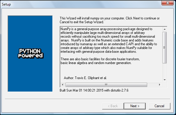
Now, we can see a description of NumPy and its features. Click on Next.
If you have Python installed, it should automatically be detected. If it is not detected, your path settings might be wrong. At the end of this chapter, we have listed resources in case you have problems with installing NumPy.
In this example, Python 2.7 was found. Click on Next if Python is found; otherwise, click on Cancel and install Python (NumPy cannot be installed without Python). Click on Next. This is the point of no return. Well, kind of, but it is best to make sure that you are installing to the proper directory and so on and so forth. Now the real installation starts. This may take a while.
Install SciPy and matplotlib with the Enthought Canopy distribution (https://www.enthought.com/products/canopy/). It might be necessary to put the
msvcp71.dllfile in yourC:\Windows\system32directory. You can get it from http://www.dll-files.com/dllindex/dll-files.shtml?msvcp71 A Windows IPython installer is available on the IPython website (see http://ipython.org/).
Installing NumPy and its related recommended software on Linux depends on the distribution you have. We will discuss how you will install NumPy from the command line, although you can probably use graphical installers; it depends on your distribution (distro). The commands to install matplotlib, SciPy, and IPython are the same—only the package names are different. Installing matplotlib, SciPy, and IPython is recommended, but optional.
Most Linux distributions have NumPy packages. We will go through the necessary commands for some of the most popular Linux distros:
Installing NumPy on Red Hat: Run the following instructions from the command line:
$ yum install python-numpyInstalling NumPy on Mandriva: To install NumPy on Mandriva, run the following command line instruction:
$ urpmi python-numpyInstalling NumPy on Gentoo: To install NumPy on Gentoo, run the following command line instruction:
$ [sudo] emerge numpyInstalling NumPy on Debian and Ubuntu: On Debian or Ubuntu, type the following on the command line:
$ [sudo] apt-get install python-numpyThe following table gives an overview of the Linux distributions and the corresponding package names for NumPy, SciPy, matplotlib, and IPython:
Linux distribution
NumPy
SciPy
matplotlib
IPython
Arch Linux
python-numpypython-scipypython-matplotlibipythonDebian
python-numpypython-scipypython-matplotlibipythonFedora
numpypython-scipypython-matplotlibipythonGentoo
dev-python/numpyscipymatplotlibipythonOpenSUSE
python-numpy, python-numpy-develpython-scipypython-matplotlibipythonSlackware
numpyscipymatplotlibipython
You can install NumPy, matplotlib, and SciPy on the Mac OS X with a GUI installer (not possible for all versions) or from the command line with a port manager such as MacPorts, Homebrew, or Fink, depending on your preference. You can also install using a script from https://github.com/fonnesbeck/ScipySuperpack.
Alternatively, we can install NumPy, SciPy, matplotlib, and IPython through the MacPorts route or with Fink. The following installation steps show how to install all these packages:
Installing with MacPorts: Type the following command:
$ [sudo] port install py-numpy py-scipy py-matplotlib py-ipythonInstalling with Fink: Fink also has packages for NumPy—
scipy-core-py24,scipy-core-py25, andscipy-core-py26. The SciPy packages arescipy-py24,scipy-py25andscipy-py26. We can install NumPy and the additional recommended packages, referring to this book on Python 2.7, using the following command:$ fink install scipy-core-py27 scipy-py27 matplotlib-py27
We can retrieve the source code for NumPy with git as follows:
$ git clone git://github.com/numpy/numpy.git numpy
Alternatively, download the source from http://sourceforge.net/projects/numpy/files/.
Install in /usr/local with the following command:
$ python setup.py build
$ [sudo] python setup.py install --prefix=/usr/local
To build, we need a C compiler such as GCC and the Python header files in the python-dev or python-devel packages.
Imagine that we want to add two vectors called a and b (see https://www.khanacademy.org/science/physics/one-dimensional-motion/displacement-velocity-time/v/introduction-to-vectors-and-scalars). Vector is used here in the mathematical sense meaning a one-dimensional array. We will learn in Chapter 5, Working with Matrices and ufuncs, about specialized NumPy arrays, which represent matrices. Vector a holds the squares of integers 0 to n, for instance, if n is equal to 3, then a is equal to (0,1, 4). Vector b holds the cubes of integers 0 to n, so if n is equal to 3, then b is equal to (0,1, 8). How will you do that using plain Python? After we come up with a solution, we will compare it to the NumPy equivalent.
Adding vectors using pure Python: The following function solves the vector addition problem using pure Python without NumPy:
def pythonsum(n):
   a = range(n)
   b = range(n)
   c = []

   for i in range(len(a)):
       a[i] = i ** 2
       b[i] = i ** 3
       c.append(a[i] + b[i])

   return c
Tip
Downloading the example code files
You can download the example code files from your account at http://www.packtpub.com for all the Packt Publishing books you have purchased. If you purchased this book elsewhere, you can visit http://www.packtpub.com/support and register to have the files e-mailed directly to you.
Adding vectors using NumPy: Following is a function that achieves the same result with NumPy:
def numpysum(n):
  a = np.arange(n) ** 2
  b = np.arange(n) ** 3
  c = a + b

  return c
Notice that numpysum() does not need a for loop. Also, we used the arange() function from NumPy that creates a NumPy array for us with integers 0 to n. The arange() function was imported; that is why it is prefixed with numpy (actually, it is customary to abbreviate it via an alias to np).
Now comes the fun part. The preface mentions that NumPy is faster when it comes to array operations. How much faster is NumPy, though? The following program will show us by measuring the elapsed time, in microseconds, for the numpysum() and pythonsum() functions. It also prints the last two elements of the vector sum. Let's check that we get the same answers by using Python and NumPy:
#!/usr/bin/env/python

from __future__ import print_function
import sys
from datetime import datetime
import numpy as np

"""
 Chapter 1 of NumPy Beginners Guide.
 This program demonstrates vector addition the Python way.
 Run from the command line as follows

  python vectorsum.py n

 where n is an integer that specifies the size of the vectors.

 The first vector to be added contains the squares of 0 up to n.
 The second vector contains the cubes of 0 up to n.
 The program prints the last 2 elements of the sum and the elapsed time.
"""

def numpysum(n):
   a = np.arange(n) ** 2
   b = np.arange(n) ** 3
   c = a + b

   return c

def pythonsum(n):
   a = range(n)
   b = range(n)
   c = []

   for i in range(len(a)):
       a[i] = i ** 2
       b[i] = i ** 3
       c.append(a[i] + b[i])

   return c


size = int(sys.argv[1])

start = datetime.now()
c = pythonsum(size)
delta = datetime.now() - start
print("The last 2 elements of the sum", c[-2:])
print("PythonSum elapsed time in microseconds", delta.microseconds)

start = datetime.now()
c = numpysum(size)
delta = datetime.now() - start
print("The last 2 elements of the sum", c[-2:])
print("NumPySum elapsed time in microseconds", delta.microseconds)
The output of the program for 1000, 2000, and 3000 vector elements is as follows:
$ python vectorsum.py 1000
The last 2 elements of the sum [995007996, 998001000]
PythonSum elapsed time in microseconds 707
The last 2 elements of the sum [995007996 998001000]
NumPySum elapsed time in microseconds 171
$ python vectorsum.py 2000
The last 2 elements of the sum [7980015996, 7992002000]
PythonSum elapsed time in microseconds 1420
The last 2 elements of the sum [7980015996 7992002000]
NumPySum elapsed time in microseconds 168
$ python vectorsum.py 4000
The last 2 elements of the sum [63920031996, 63968004000]
PythonSum elapsed time in microseconds 2829
The last 2 elements of the sum [63920031996 63968004000]
NumPySum elapsed time in microseconds 274
Clearly, NumPy is much faster than the equivalent normal Python code. One thing is certain, we get the same results whether we use NumPy or not. However, the result printed differs in representation. Notice that the result from the numpysum() function does not have any commas. How come? Obviously, we are not dealing with a Python list but with a NumPy array. It was mentioned in the Preface that NumPy arrays are specialized data structures for numerical data. We will learn more about NumPy arrays in the next chapter.
Q1. What does arange(5) do?
Creates a Python list of 5 elements with the values 1-5.
Creates a Python list of 5 elements with the values 0-4.
Creates a NumPy array with the values 1-5.
Creates a NumPy array with the values 0-4.
None of the above.
The program we used to compare the speed of NumPy and regular Python is not very scientific. We should at least repeat each measurement a couple of times. It will be nice to be able to calculate some statistics such as average times. Also, you might want to show plots of the measurements to friends and colleagues.
Tip
Hints to help can be found in the online documentation and the resources listed at the end of this chapter. NumPy has statistical functions that can calculate averages for you. I recommend using matplotlib to produce plots. Chapter 9, Plotting with matplotlib, gives a quick overview of matplotlib.
Scientists and engineers are used to experiment. Scientists created IPython with experimentation in mind. Many view the interactive environment that IPython provides as a direct answer to MATLAB, Mathematica, and Maple. You can find more information, including installation instructions, at http://ipython.org/.
IPython is free, open source, and available for Linux, UNIX, Mac OS X, and Windows. The IPython authors only request that you cite IPython in any scientific work that uses IPython. The following is a list of the basic IPython features:
Tab completion
History mechanism
Inline editing
Ability to call external Python scripts with %run
Access to system commands
Pylab switch
Access to Python debugger and profiler
The Pylab switch imports all the SciPy, NumPy, and matplotlib packages. Without this switch, we will have to import every package we need ourselves.
All we need to do is enter the following instruction on the command line:
$ ipython --pylab
IPython 2.4.1 -- An enhanced Interactive Python.
?         -> Introduction and overview of IPython's features.
%quickref -> Quick reference.
help      -> Python's own help system.
object?   -> Details about 'object', use 'object??' for extra details.
Using matplotlib backend: MacOSX

In [1]: quit()
The quit()command or Ctrl + D quits the IPython shell. We may want to be able to go back to our experiments. In IPython, it is easy to save a session for later:
In [1]: %logstart
Activating auto-logging. Current session state plus future input saved.
Filename       : ipython_log.py
Mode           : rotate
Output logging : False
Raw input log  : False
Timestamping   : False
State          : active
Let's say we have the vector addition program that we made in the current directory. Run the script as follows:
In [1]: ls
README        vectorsum.py
In [2]: %run -i vectorsum.py 1000
As you probably remember, 1000 specifies the number of elements in a vector. The -d switch of %run starts an ipdb debugger with c the script is started. n steps through the code. Typing quit at the ipdb prompt exits the debugger:
In [2]: %run -d vectorsum.py 1000
*** Blank or comment
*** Blank or comment
Breakpoint 1 at: /Users/…/vectorsum.py:3
><string>(1)<module>()
ipdb> c
> /Users/…/vectorsum.py(3)<module>()
      2
1---> 3 import sys
      4 from datetime import datetime
ipdb> n
>
/Users/…/vectorsum.py(4)<module>()
1     3 import sys
----> 4 from datetime import datetime
      5 import numpy
ipdb> n
> /Users/…/vectorsum.py(5)<module>()
      4 from datetime import datetime
----> 5 import numpy
      6
ipdb> quit
We can also profile our script by passing the -p option to %run:
In [4]: %run -p vectorsum.py 1000
         1058 function calls (1054 primitive calls) in 0.002 CPU seconds
   Ordered by: internal time
ncalls tottime percall cumtime percall filename:lineno(function)
1 0.001    0.001   0.001    0.001 vectorsum.py:28(pythonsum)
1 0.001    0.001   0.002    0.002 {execfile}
1000 0.000    0.0000.0000.000 {method 'append' of 'list' objects}
1 0.000    0.000    0.002    0.002 vectorsum.py:3(<module>)
1 0.000    0.0000.0000.000 vectorsum.py:21(numpysum)
3    0.000    0.0000.0000.000 {range}
1    0.000    0.0000.0000.000 arrayprint.py:175(_array2string)
3/1    0.000    0.0000.0000.000 arrayprint.py:246(array2string)
2    0.000    0.0000.0000.000 {method 'reduce' of 'numpy.ufunc' objects}
4    0.000    0.0000.0000.000 {built-in method now}
2    0.000    0.0000.0000.000 arrayprint.py:486(_formatInteger)
2    0.000    0.0000.0000.000 {numpy.core.multiarray.arange}
1    0.000    0.0000.0000.000 arrayprint.py:320(_formatArray)
3/1    0.000    0.0000.0000.000 numeric.py:1390(array_str)
1    0.000    0.0000.0000.000 numeric.py:216(asarray)
2    0.000    0.0000.0000.000 arrayprint.py:312(_extendLine)
1    0.000    0.0000.0000.000 fromnumeric.py:1043(ravel)
2    0.000    0.0000.0000.000 arrayprint.py:208(<lambda>)
1    0.000    0.000    0.002    0.002<string>:1(<module>)
11    0.000    0.0000.0000.000 {len}
2    0.000    0.0000.0000.000 {isinstance}
1    0.000    0.0000.0000.000 {reduce}
1    0.000    0.0000.0000.000 {method 'ravel' of 'numpy.ndarray' objects}
4    0.000    0.0000.0000.000 {method 'rstrip' of 'str' objects}
3    0.000    0.0000.0000.000 {issubclass}
2    0.000    0.0000.0000.000 {method 'item' of 'numpy.ndarray' objects}
1    0.000    0.0000.0000.000 {max}
1    0.000    0.0000.0000.000 {method 'disable' of '_lsprof.Profiler' objects}
This gives us a bit more insight in to the workings of our program. In addition, we can now identify performance bottlenecks. The %hist command shows the commands history:
In [2]: a=2+2
In [3]: a
Out[3]: 4
In [4]: %hist
1: _ip.magic("hist ")
2: a=2+2
3: a
I hope you agree that IPython is a really useful tool!
When we are in IPython's pylab mode, we can open manual pages for NumPy functions with the help command. It is not necessary to know the name of a function. We can type a few characters and then let tab completion do its work. Let's, for instance, browse the available information for the arange() function:
In [2]: help ar<Tab>
In [2]: help arange
Another option is to put a question mark behind the function name:
In [3]: arange?
The main documentation website for NumPy and SciPy is at http://docs.scipy.org/doc/. Through this web page, we can browse the NumPy reference at http://docs.scipy.org/doc/numpy/reference/, the user guide, and several tutorials.
The popular Stack Overflow software development forum has hundreds of questions tagged numpy. To view them, go to http://stackoverflow.com/questions/tagged/numpy.
If you are really stuck with a problem or you want to be kept informed of NumPy development, you can subscribe to the NumPy discussion mailing list. The e-mail address is <numpy-discussion@scipy.org>. The number of e-mails per day is not too high with almost no spam to speak of. Most importantly, the developers actively involved with NumPy also answer questions asked on the discussion group. The complete list can be found at http://www.scipy.org/scipylib/mailing-lists.html.
For IRC users, there is an IRC channel on irc://irc.freenode.net. The channel is called #scipy, but you can also ask NumPy questions since SciPy users also have knowledge of NumPy, as SciPy is based on NumPy. There are at least 50 members on the SciPy channel at all times.
In this chapter, we installed NumPy and other recommended software that we will be using in some sections of this book. We got a vector addition program working and convinced ourselves that NumPy has superior performance. You were introduced to the IPython interactive shell. In addition, you explored the available NumPy documentation and online resources.
In the next chapter, you will take a look under the hood and explore some fundamental concepts including arrays and data types.