


 Download code from GitHub
In this chapter, you will start your journey toward mastery of parallelism in R by quickly learning to exploit the multicore processing capability of your own laptop and travel onward to our first look at how you can most simply exploit the vast computing capacity of the cloud.
You will learn about lapply() and its variations supported by R's core parallel package as well as about the segue package that enables us to utilize Amazon Web Services (AWS) and the Elastic Map Reduce (EMR) service. For the latter, you will need to have an account set up with AWS.
Our worked example throughout this chapter will be an iterative solver for an ancient puzzle known as Aristotle's Number Puzzle. Hopefully, this will be something new to you and pique your interest. It has been specifically chosen to demonstrate an important issue that can arise when running code in parallel, namely imbalanced computation. It will also serve to help develop our performance benchmarking skills—an important consideration in parallelism—measuring overall computational effectiveness.
The examples in this chapter are developed using RStudio version 0.98.1062 with the 64-bit R version 3.1.0 (CRAN distribution) running on a mid-2014 generation Apple MacBook Pro OS X 10.9.4 with a 2.6 GHz Intel Core i5 processor and 16 GB memory. Some of the examples in this chapter will not be able to run with Microsoft Windows, but should run without problem on all variants of Linux.
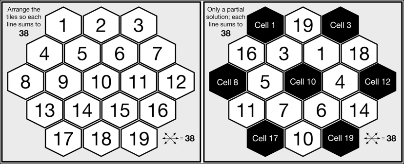
The puzzle we will solve is known as Aristotle's Number Puzzle, and this is a magic hexagon. The puzzle requires us to place 19 tiles, numbered 1 to 19, on a hexagonal grid such that each horizontal row and each diagonal across the board adds up to 38 when summing each of the numbers on each of the tiles in the corresponding line. The following, on the left-hand side, is a pictorial representation of the unsolved puzzle showing the hexagonal grid layout of the board with the tiles placed in order from the upper-left to the lower-right. Next to this, a partial solution to the puzzle is shown, where the two rows (starting with the tiles 16 and 11) and the four diagonals all add up to 38, with empty board cells in the positions 1, 3, 8, 10, 12, 17, and 19 and seven remaining unplaced tiles, 2, 8, 9, 12, 13, 15, and 17:
The mathematically minded among you will already have noticed that the number of possible tile layouts is the factorial 19; that is, there is a total of 121,645,100,408,832,000 unique combinations (ignoring rotational and mirror symmetry). Even when utilizing a modern microprocessor, it will clearly take a considerable period of time to find which of these 121 quadrillion combinations constitute a valid solution.
The algorithm we will use to solve the puzzle is a depth-first iterative search, allowing us to trade off limited memory for compute cycles; we could not feasibly store every possible board configuration without incurring huge expense.
Let's start our implementation by considering how to represent the board. The simplest way is to use a one-dimensional R vector of length 19, where the index i of the vector represents the corresponding ith cell on the board. Where a tile is not yet placed, the value of the board vector's "cell" will be the numeric 0.
empty_board   <- c(0,0,0,0,0,0,0,0,0,0,0,0,0,0,0,0,0,0,0)
partial_board <- c(0,19,0,16,3,1,18,0,5,0,4,0,11,7,6,14,0,10,0)
Next, let's define a function to evaluate whether the layout of tiles on the board represents a valid solution. As part of this, we need to specify the various combinations of board cells or "lines" that must add up to the target value 38, as follows:
all_lines <- list(
  c(1,2,3),        c(1,4,8),        c(1,5,10,15,19),
  c(2,5,9,13),     c(2,6,11,16),    c(3,7,12),
  c(3,6,10,14,17), c(4,5,6,7),      c(4,9,14,18),
  c(7,11,15,18),   c(8,9,10,11,12), c(8,13,17),
  c(12,16,19),     c(13,14,15,16),  c(17,18,19)
)
evaluateBoard <- function(board)
{
  for (line in all_lines) {
    total <- 0
    for (cell in line) {
      total <- total + board[cell]
    }
    if (total != 38) return(FALSE)
  }
  return(TRUE) # We have a winner!
}
In order to implement the depth-first solver, we need to manage the list of remaining tiles for the next tile placement. For this, we will utilize a variation on a simple stack by providing push and pop functions for both the first and last item within a vector. To make this distinct, we will implement it as a class and call it sequence.
Here is a simple S3-style class sequence that implements a double-ended head/tail stack by internally maintaining the stack's state within a vector:
  sequence <- function()
  {
    sequence <- new.env()      # Shared state for class instance
    sequence$.vec <- vector()  # Internal state of the stack
    sequence$getVector <- function() return (.vec)
    sequence$pushHead <- function(val) .vec <<- c(val, .vec)
    sequence$pushTail <- function(val) .vec <<- c(.vec, val)
    sequence$popHead <- function() {
      val <- .vec[1]
      .vec <<- .vec[-1]        # Update must apply to shared state
      return(val)
    }
    sequence$popTail <- function() {
      val <- .vec[length(.vec)]
      .vec <<- .vec[-length(.vec)]
      return(val)
    }
    sequence$size <- function() return( length(.vec) )
    # Each sequence method needs to use the shared state of the
    # class instance, rather than its own function environment
    environment(sequence$size)      <- as.environment(sequence)
    environment(sequence$popHead)   <- as.environment(sequence)
    environment(sequence$popTail)   <- as.environment(sequence)
    environment(sequence$pushHead)  <- as.environment(sequence)
    environment(sequence$pushTail)  <- as.environment(sequence)
    environment(sequence$getVector) <- as.environment(sequence)
    class(sequence) <- "sequence"
    return(sequence)
  }
The implementation of the sequence should be easy to understand from some example usage, as in the following:
> s <- sequence()     ## Create an instance s of sequence
> s$pushHead(c(1:5))  ## Initialize s with numbers 1 to 5
> s$getVector()
[1] 1 2 3 4 5
> s$popHead()         ## Take the first element from s
[1] 1
> s$getVector()       ## The number 1 has been removed from s
[1] 2 3 4 5
> s$pushTail(1)       ## Add number 1 as the last element in s
> s$getVector()
[1] 2 3 4 5 1
We are almost there. Here is the implementation of the placeTiles() function to perform the depth-first search:
  01 placeTiles <- function(cells,board,tilesRemaining)
  02 {
  03  for (cell in cells) {
  04    if (board[cell] != 0) next # Skip cell if not empty
  05    maxTries <- tilesRemaining$size()
  06    for (t in 1:maxTries) {
  07      board[cell] = tilesRemaining$popHead()
  08      retval <- placeTiles(cells,board,tilesRemaining)
  09      if (retval$Success) return(retval)
  10      tilesRemaining$pushTail(board[cell])
  11    }
  12    board[cell] = 0 # Mark this cell as empty
  13    # All available tiles for this cell tried without success
  14    return( list(Success = FALSE, Board = board) )
  15  }
  16  success <- evaluateBoard(board)
  17  return( list(Success = success, Board = board) )
  18 }
The function exploits recursion to place each subsequent tile on the next available cell. As there are a maximum of 19 tiles to place, recursion will descend to a maximum of 19 levels (Line 08). The recursion will bottom out when no tiles remain to be placed on the board, and the board will then be evaluated (Line 16). A successful evaluation will immediately unroll the recursion stack (Line 09), propagating the final completed state of the board to the caller (Line 17). An unsuccessful evaluation will recurse one step back up the calling stack and cause the next remaining tile to be tried instead. Once all the tiles are exhausted for a given cell, the recursion will unroll to the previous cell, the next tile in the sequence will be tried, the recursion will progress again, and so on.
Usefully, the placeTiles() function enables us to test a partial solution, so let's try out the partial tile placement from the beginning of this chapter. Execute the following code:
> board <- c(0,19,0,16,3,1,18,0,5,0,4,0,11,7,6,14,0,10,0)
> tiles <- sequence()
> tiles$pushHead(c(2,8,9,12,13,15,17))
> cells <- c(1,3,8,10,12,17,19)
> placeTiles(cells,board,tiles)
$Success
[1] FALSE
$Board
[1]  0 19  0 16  3  1 18  0  5  0  4  0 11  7  6 14  0 10  0
Tip
Downloading the example code
You can download the example code files for this book from your account at http://www.packtpub.com. If you purchased this book elsewhere, you can visit http://www.packtpub.com/support and register to have the files e-mailed directly to you.
You can download the code files by following these steps:
Log in or register to our website using your e-mail address and password.
Hover the mouse pointer on the SUPPORT tab at the top.
Click on Code Downloads & Errata.
Enter the name of the book in the Search box.
Select the book for which you're looking to download the code files.
Choose from the drop-down menu where you purchased this book from.
Click on Code Download.
You can also download the code files by clicking on the Code Files button on the book's webpage at the Packt Publishing website. This page can be accessed by entering the book's name in the Search box. Please note that you need to be logged in to your Packt account.
Once the file is downloaded, please make sure that you unzip or extract the folder using the latest version of:
WinRAR / 7-Zip for Windows
Zipeg / iZip / UnRarX for Mac
7-Zip / PeaZip for Linux
The code bundle for the book is also hosted on GitHub at https://github.com/PacktPublishing/repository-name. We also have other code bundles from our rich catalog of books and videos available at https://github.com/PacktPublishing/. Check them out!
Unfortunately, our partial solution does not yield a complete solution.
We'll clearly have to try a lot harder.
Before we jump into parallelizing our solver, let's first examine the efficiency of our current serial implementation. With the existing placeTiles() implementation, the tiles are laid until the board is complete, and then it is evaluated. The partial solution we tested previously, with seven cells unassigned, required 7! = 5,040 calls to evaluateBoard() and a total of 13,699 tile placements.
The most obvious refinement we can make is to test each tile as we place it and check whether the partial solution up to this point is correct rather than waiting until all the tiles are placed. Intuitively, this should significantly reduce the number of tile layouts that we have to explore. Let's implement this change and then compare the difference in performance so that we understand the real benefit from doing this extra implementation work:
  cell_lines <- list(
    list( c(1,2,3),    c(1,4,8),    c(1,5,10,15,19) ), #Cell 1
 .. # Cell lines 2 to 18 removed for brevity
    list( c(12,16,19), c(17,18,19), c(1,5,10,15,19) )  #Cell 19
  )
  evaluateCell <- function(board,cellplaced)
  {
    for (lines in cell_lines[cellplaced]) {
      for (line in lines) {
        total <- 0
        checkExact <- TRUE
        for (cell in line) {
          if (board[cell] == 0) checkExact <- FALSE
          else total <- total + board[cell]
        }
        if ((checkExact && (total != 38)) || total > 38)
          return(FALSE)
      }
    }
    return(TRUE)
  }
For efficiency, the evaluateCell() function determines which lines need to be checked based on the cell that is just placed by performing direct lookup against cell_lines. The cell_lines data structure is easily compiled from all_lines (you could even write some simple code to generate this). Each cell on the board requires three specific lines to be tested. As any given line being tested may not be filled with tiles, evaluateCell() includes a check to ensure that it only applies the 38 sum test when a line is complete. For a partial line, a check is made to ensure that the sum does not exceed 38.
We can now augment placeTiles() to call evaluateCell() as follows:
  01 placeTiles <- function(cells,board,tilesRemaining)
  ..
  06    for (t in 1:maxTries) {
  07      board[cell] = tilesRemaining$popHead()
  ++      if (evaluateCell(board,cell)) {
  08        retval <- placeTiles(cells,board,tilesRemaining)
  09        if (retval$Success) return(retval)
  ++      }
  10      tilesRemaining$pushTail(board[cell])
  11    }
..Before we apply this change, we need to first benchmark the current placeTiles() function so that we can determine the resulting performance improvement. To do this, we'll introduce a simple timing function, teval(), that will enable us to measure accurately how much work the processor does when executing a given R function. Take a look at the following:
  teval <- function(...) {
    gc(); # Perform a garbage collection before timing R function
    start <- proc.time()
    result <- eval(...)
    finish <- proc.time()
    return ( list(Duration=finish-start, Result=result) )
  }
The teval() function makes use of an internal system function, proc.time(), to record the current consumed user and system cycles as well as the wall clock time for the R process [unfortunately, this information is not available when R is running on Windows]. It captures this state both before and after the R expression being measured is evaluated and computes the overall duration. To help ensure that there is a level of consistency in timing, a preemptive garbage collection is invoked, though it should be noted that this does not preclude R from performing a garbage collection at any further point during the timing period.
So, let's run teval() on the existing placeTiles() as follows:
> teval(placeTiles(cells,board,tiles))
$Duration
   user  system elapsed
  0.421   0.005   0.519
$Result
..
Now, let's make the changes in placeTiles() to call evaluateCell() and run it again via the following code:
> teval(placeTiles(cells,board,tiles))
$Duration
   user  system elapsed
  0.002   0.000   0.002
$Result
..
This is a nice result! This one change has significantly reduced our execution time by a factor of 200. Obviously, your own absolute timings may vary based on the machine you use.
Tip
Benchmarking code
For true comparative benchmarking, we should run tests multiple times and from a full system startup for each run to ensure there are no caching effects or system resource contention issues taking place that might skew our results. For our specific simple example code, which does not perform file I/O or network communications, handle user input, or use large amounts of memory, we should not encounter these issues. Such issues will typically be indicated by significant variation in time taken over multiple runs, a high percentage of system time or the elapsed time being substantively greater than the user + system time.
This kind of performance profiling and enhancement is important as later in this chapter, we will pay directly for our CPU cycles in the cloud; therefore, we want our code to be as cost effective as possible.
For a little deeper understanding of the behavior of our code, such as how many times a function is called during program execution, we either need to add explicit instrumentation, such as counters and print statements, or use external tools such as Rprof. For now, though, we will take a quick look at how we can apply the base R function trace() to provide a generic mechanism to profile the number of times a function is called, as follows:
  profileFn <- function(fn)       ## Turn on tracing for "fn"
  {
    assign("profile.counter",0,envir=globalenv())
    trace(fn,quote(assign("profile.counter",
                    get("profile.counter",envir=globalenv()) + 1,
                   envir=globalenv())), print=FALSE)
  }
  profileFnStats <- function(fn)  ## Get collected stats
  {
    count <- get("profile.counter",envir=globalenv())
    return( list(Function=fn,Count=count) )
  }
  unprofileFn <- function(fn)     ## Turn off tracing and tidy up
  {
    remove(list="profile.counter",envir=globalenv())
    untrace(fn)
  }
The trace() function enables us to execute a piece of code each time the function being traced is called. We will exploit this to update a specific counter we create (profile.counter) in the global environment to track each invocation.
Note
trace()
This function is only available when the tracing is explicitly compiled into R itself. If you are using the CRAN distribution of R for either Mac OS X or Microsoft Windows, then this facility will be turned on. Tracing introduces a modicum of overhead even when not being used directly within code and therefore tends not to be compiled into R production environments.
We can demonstrate profileFn() working in our running example as follows:
> profile.counter
Error: object 'profile.counter' not found
> profileFn("evaluateCell")
[1] "evaluateCell"
> profile.counter
[1] 0
> placeTiles(cells,board,tiles)
..
> profileFnStats("evaluateCell")
$Function
[1] "evaluateCell"
$Count
[1] 59
> unprofileFn("evaluateCell")
> profile.counter
Error: object 'profile.counter' not found
What this result shows is that evaluateCell() is called 59 times as compared to our previous evaluateBoard() function, which was called 5,096 times. This accounts for the significantly reduced runtime and combinatorial search space that must be explored.
Parallelism relies on being able to split a problem into separate units of work. Trivial—or as it is sometimes referred to, naïve parallelism—treats each separate unit of work as entirely independent of one another. Under this scheme, while a unit of work, or task, is being processed, there is no requirement for the computation to interact with or share information with other tasks being computed, either now, previously, or subsequently.
For our number puzzle, an obvious approach would be to split the problem into 19 separate tasks, where each task is a different-numbered tile placed at cell 1 on the board, and the task is to explore the search space to find a solution stemming from the single tile starting position. However, this only gives us a maximum parallelism of 19, meaning we can explore our search space a maximum of 19 times faster than in serial. We also need to consider our overall efficiency. Does each of the starting positions result in the same amount of required computation? In short, no; as we will use a depth-first algorithm in which a correct solution found will immediately end the task in contrast to an incorrect starting position that will likely result in a much larger, variable, and inevitably fruitless search space being explored. Our tasks are therefore not balanced and will require differing amounts of computational effort to complete. We also cannot predict which of the tasks will take longer to compute as we do not know which starting position will lead to the correct solution a priori.
Note
Imbalanced computation
This type of scenario is typical of a whole host of real-world problems where we search for an optimal or near-optimal solution in a complex search space—for example, finding the most efficient route and means of travel around a set of destinations or planning the most efficient use of human and building resources when timetabling a set of activities. Imbalanced computation can be a significant problem where we have a fully committed compute resource and are effectively waiting for the slowest task to be performed before the overall computation can complete. This reduces our parallel speed-up in comparison to running in serial, and it may also mean that the compute resource we are paying for spends a significant period of time idle rather than doing useful work.
To increase our overall efficiency and opportunity for parallelism, we will split the problem into a larger number of smaller computational tasks, and we will exploit a particular feature of the puzzle to significantly reduce our overall search space.
We will generate the starting triple of tiles for the first (top) line of the board, cells 1 to 3. We might expect that this will give us 19x18x17 = 5,814 tile combinations. However, only a subset of these tile combinations will sum to 38; 1+2+3 and 17+18+19 clearly are not valid. We can also filter out combinations that are a mirror image; for example, for the first line of the board, 1+18+19 will yield an equivalent search space to 19+18+1, so we only need to explore one of them.
Here is the code for generateTriples(). You will notice that we are making use of a 6-character string representation of a tile-triple to simplify the mirror image test, and it also happens to be a reasonably compact and efficient implementation:
  generateTriples <- function()
  {
    triples <- list()
    for (x in 1:19) {
      for (y in 1:19) {
        if (y == x) next
        for (z in 1:19) {
          if (z == x || z == y || x+y+z != 38) next
          mirror <- FALSE
          reversed <- sprintf("%02d%02d%02d",z,y,x)
          for (t in triples) {
            if (reversed == t) {
              mirror <- TRUE
              break
            }
          }
          if (!mirror) {
            triples[length(triples)+1] <-
                      sprintf("%02d%02d%02d",x,y,z)
          }
        }
      }
    }
    return (triples)
  }
If we run this, we will generate just 90 unique triples, a significant saving over 5,814 starting positions:
> teval(generateTriples())
$Duration
   user  system elapsed
  0.025   0.001   0.105
$Result[[1]]
[1] "011819"
  ..
$Result[[90]]
[1] "180119"
Now that we have an efficiently defined set of board starting positions, we can look at how we can manage the set of tasks for distributed computation. Our starting point will be lapply() as this enables us to test out our task execution and formulate it into a program structure, for which we can do a simple drop-in replacement to run in parallel.
The lapply() function takes two arguments, the first is a list of objects that act as input to a user-defined function, and the second is the user-defined function to be called, once for each separate input object; it will return the collection of results from each function invocation as a single list. We will repackage our solver implementation to make it simpler to use with lapply() by wrapping up the various functions and data structures we developed thus far in an overall solver() function, as follows (the complete source code for the solver is available on the book's website):
  solver <- function(triple)
  {
    all_lines <- list(..
    cell_lines <- list(..
    sequence <- function(..
    evaluateBoard <- function(..
    evaluateCell <- function(..
    placeTiles <- function(..
    teval <- function(..

    ## The main body of the solver
    tile1 <- as.integer(substr(triple,1,2))
    tile2 <- as.integer(substr(triple,3,4))
    tile3 <- as.integer(substr(triple,5,6))
    board <- c(tile1,tile2,tile3,0,0,0,0,0,0,0,0,0,0,0,0,0,0,0,0)
    cells <- c(4,5,6,7,8,9,10,11,12,13,14,15,16,17,18,19)
    tiles <- sequence()
    for (t in 1:19) {
      if (t == tile1 || t == tile2 || t == tile3) next
      tiles$pushHead(t)
    }
    result <- teval(placeTiles(cells,board,tiles))
    return( list(Triple = triple, Result = result$Result,
                  Duration= result$Duration) )
  }
Let's run our solver with a selection of four of the tile-triples:
> tri <- generateTriples()
> tasks <- list(tri[[1]],tri[[21]],tri[[41]],tri[[61]])
> teval(lapply(tasks,solver))
$Duration               ## Overall
   user  system elapsed
171.934   0.216 172.257
$Result[[1]]$Duration   ## Triple "011819"
   user  system elapsed
  1.113   0.001   1.114
$Result[[2]]$Duration   ## Triple "061517"
   user  system elapsed
 39.536   0.054  39.615
$Result[[3]]$Duration   ## Triple "091019"
   user  system elapsed
 65.541   0.089  65.689
$Result[[4]]$Duration   ## Triple "111215"
   user  system elapsed
 65.609   0.072  65.704
The preceding output has been trimmed and commented for brevity and clarity. The key thing to note is that there is significant variation in the time (the elapsed time) it takes on my laptop to run through the search space for each of the four starting tile-triples, none of which happen to result in a solution to the puzzle. We can (perhaps) project from this that it will take at least 90 minutes to run through the complete set of triples if running in serial. However, we can solve the puzzle much faster if we run our code in parallel; so, without further ado….
The R parallel package is now part of the core distribution of R. It includes a number of different mechanisms to enable you to exploit parallelism utilizing the multiple cores in your processor(s) as well as compute the resources distributed across a network as a cluster of machines. However, as our theme in this chapter is one of simplicity, we will stick to making the most of the resources available on the machine on which you are running R.
The first thing you need to do is to enable the parallelism package. You can either just use R's library() function to load it, or if you are using RStudio, you can just tick the corresponding entry in the User Library list in the Packages tab. The second thing we need to do is determine just how much parallelism we can utilize by calling the parallel package function detectCores(), as follows:
> library("parallel")
> detectCores()
[1] 4
As we can immediately note, on my MacBook device, I have four cores available across which I can run R programs in parallel. It's easy to verify this using Mac's Activity Monitor app and selecting the CPU History option from the Window menu. You should see something similar to the following, with one timeline graph per core:
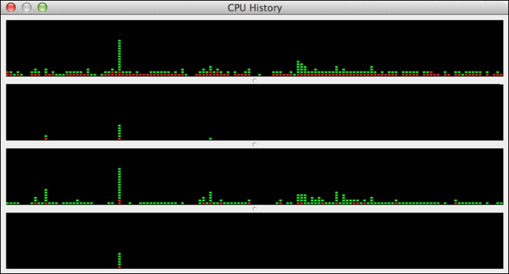
The green elements of the plotted bars indicate the proportion of CPU spent in user code, and the red elements indicate the proportion of time spent in system code. You can vary the frequency of graph update to a maximum of once a second. A similar multicore CPU history is available in Microsoft Windows. It is useful to have this type of view open when running code in parallel as you can immediately see when your code is utilizing multiple cores. You can also see what other activity is taking place on your machine that might impact your R code running in parallel.
The simplest mechanism to achieve parallelism in R is to use parallel's multicore variant of lapply() called (logically) mclapply().
Note
The mclapply() function is Unix-only
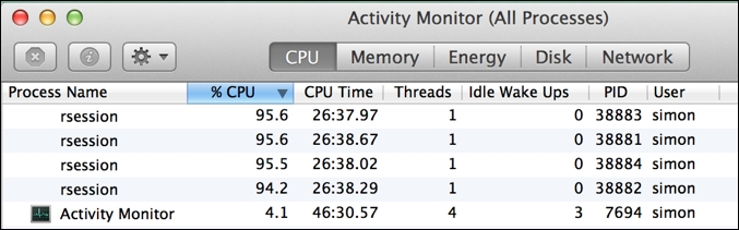
The mclapply() function is only available when you are running R on Mac OS X or Linux or other variants of Unix. It is implemented with the Unix fork() system call and therefore cannot be used on Microsoft Windows; rest assured, we will come to a Microsoft Windows compatible solution shortly. The Unix fork() system call operates by replicating the currently running process (including its entire memory state, open file descriptors, and other process resources, and importantly, from an R perspective, any currently loaded libraries) as a set of independent child processes that will each continue separate execution until they make the exit() system call, at which point the parent process will collect their exit state. Once all children terminate, the fork will be completed. All of this behavior is wrapped up inside the call to mclapply(). If you view your running processes in Activity Monitor on Mac OS X, you will see mc.cores number of spawned rsession processes with high CPU utilization when mclapply() is called.
Similar to lapply(), the first argument is the list of function inputs corresponding to independent tasks, and the second argument is the function to be executed for each task. An optional argument, mc.cores, allows us to specify how many cores we want to make use of—that is, the degree of parallelism we want to use. If when you ran detectCores() and the result was 1, then mclapply() will resort to just calling lapply() internally—that is, the computation will just run serially.
Let's initially run
mclapply() through a small subset of the triple tile board starting positions using the same set we tried previously with lapply() for comparison, as follows:
> tri <- generateTriples()
> tasks <- list(tri[[1]],tri[[21]],tri[[41]],tri[[61]])
> teval(mclapply(tasks,solver,mc.cores=detectCores()))
$Duration               ## Overall
   user  system elapsed
146.412   0.433  87.621
$Result[[1]]$Duration   ## Triple "011819"
   user  system elapsed
  2.182   0.010   2.274
$Result[[2]]$Duration   ## Triple "061517"
   user  system elapsed
 58.686   0.108  59.391
$Result[[3]]$Duration   ## Triple "091019"
   user  system elapsed
 85.353   0.147  86.198
$Result[[4]]$Duration   ## Triple "111215"
   user  system elapsed
 86.604   0.152  87.498
The preceding output is again trimmed and commented for brevity and clarity. What you should immediately notice is that the overall elapsed time for executing all of the tasks is no greater than the length of time it took to compute the longest running of the four tasks. Voila! We have managed to significantly reduce our running time from 178 seconds running in serial to just 87 seconds by making simultaneous use of all the four cores available. However, 87 seconds is only half of 178 seconds, and you may have expected that we would have seen a four-times speedup over running in serial. You may also notice that our individual runtime increased for each individual task compared to running in serial—for example, for tile-triple 111215 from 65 seconds to 87 seconds. Part of this difference is due to the overhead from the forking mechanism and the time it takes to spin up a new child process, apportion it tasks, collect its results, and tear it down. The good news is that this overhead can be amortized by having each parallel process compute a large number of tasks.
Another consideration is that my particular MacBook laptop uses an Intel Core i5 processor, which, in practice, is more the equivalent of 2 x 1.5 cores as it exploits hyperthreading across two full processor cores to increase performance and has certain limitations but is still treated by the operating system as four fully independent cores. If I run the preceding example on two of my laptop cores, then the overall runtime is just 107 seconds. Two times hyperthreading, therefore, gains me an extra 20% on performance, which although good, is still much less than the desired 50% performance improvement.
I'm sure at this point, if you haven't already done so, then you will have the urge to run the solver in parallel across all 90 of the starting tile-triples and find the solution to Aristotle's Number Puzzle, though you might want to take a long coffee break or have lunch while it runs….
The
mclapply() function has more capability than we have so far touched upon. The following table summarizes these extended capabilities and briefly discusses when they are most appropriately applied:
mclapply(X, FUN, ..., mc.preschedule=TRUE, mc.set.seed=TRUE,
         mc.silent=FALSE, mc.cores=getOption("mc.cores",2L),
         mc.cleanup=TRUE, mc.allow.recursive=TRUE)
returns: list of FUN results, where length(returns)=length(X)Tip
The print() function in parallel
In Rstudio, the output is not directed to the screen when running in parallel with mclapply(). If you wish to generate print messages or other console output, you should run your program directly from the command shell rather than from within RStudio. In general, the authors of mclapply() do not recommend running parallel R code from a GUI console editor because it can cause a number of complications, with multiple processes attempting to interact with the GUI. It is not suitable, for example, to attempt to plot to the GUI's graphics display when running in parallel. With our solver code, though, you should not experience any specific issue. It's also worth noting that having multiple processes writing messages to the same shared output stream can become very confusing as messages can potentially be interleaved and unreadable, depending on how the output stream buffers I/O. We will come back to the topic of parallel I/O in a later chapter.
The
mclapply() function is closely related to the more generic parallel package function parLapply(). The key difference is that we separately create a cluster of parallel R processes using makeCluster(), and parLapply() then utilizes this cluster when executing a function in parallel. There are two key advantages to this approach. Firstly, with makeCluster(), we can create different underlying implementations of a parallel processing pool, including a forked process cluster (FORK) similar to that used internally within mclapply(), a socket-based cluster (PSOCK) that will operate on Microsoft Windows as well as OS X and Linux, and a message-passing-based cluster (MPI), whichever is best suited to our circumstances. Secondly, the overhead of creating and configuring the cluster (we will visit the R configuration of the cluster in a later chapter) is amortized as it can be continually reused within our session.
The PSOCK and MPI types of cluster also enable R to utilize multiple machines within a network and perform true distributed computing (the machines may also be running different operating systems). However, for now, we will focus on the PSOCK cluster type and how this can be utilized within a single machine context. We will explore MPI in detail in Chapter 2, Introduction to MessagePassing, Chapter 3, Advanced Message Passing, Chapter 4, Developing SPRINT an MPI-based Package for Supercomputers.
Let's jump right in; run the following:
> cluster <- makeCluster(detectCores(),"PSOCK")

> tri <- generateTriples()
> tasks <- list(tri[[1]],tri[[21]],tri[[41]],tri[[61]])
> teval(parLapply(cluster,tasks,solver))
$Duration               ## Overall
   user  system elapsed
  0.119   0.148  83.820
$Result[[1]]$Duration   ## Triple "011819"
   user  system elapsed
  2.055   0.008   2.118
$Result[[2]]$Duration   ## Triple "061517"
   user  system elapsed
 55.603   0.156  56.749
$Result[[3]]$Duration   ## Triple "091019"
   user  system elapsed
 81.949   0.208  83.195
$Result[[4]]$Duration   ## Triple "111215"
   user  system elapsed
 82.591   0.196  83.788

> stopCluster(cluster)  ## Shutdown the cluster (reap processes)
What you may immediately notice from the timing results generated before is that the overall user time is recorded as negligible. This is because in the launching process, your main R session (referred to as the master) does not perform any of the computation, and all of the computation is carried out by the cluster. The master merely has to send out the tasks to the cluster and wait for the results to return.
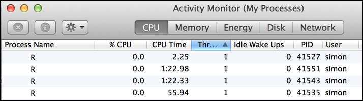
What's also particularly apparent when running a cluster in this mode is the imbalance in computation across the processes in the cluster (referred to as workers). As the following image demonstrates very clearly, each R worker process in the cluster computed a single task in variable time, and the PID 41527 process sat idle after just two seconds while the PID 41551 process was busy still computing its task for a further 1m 20s:
While increasing the number of tasks for the cluster to perform and assuming a random assignment of tasks to workers should increase efficiency, we still could end up with a less-than optimal overall utilization of resource. What we need is something more adaptive that hands out tasks dynamically to worker processes whenever they are next free to do more work. Luckily for us, there is a variation on parLapply() that does just this….
Note
Other parApply functions
There is a whole family of cluster functions to suit different types of workload, such as processing R matrices in parallel. These are summarized briefly here:
parSapply(): This is the parallel variant ofsapply()that simplifies the return type (if possible) to a choice of vector, matrix, or array.parCapply(),parRapply(): These are the parallel operations that respectively apply to the columns and rows of a matrix.parLapplyLB(),parSapplyLB(): These are the load-balancing versions of their similarly named cousins. Load balancing is discussed in the next section.clusterApply(),clusterApplyLB(): These are generic apply and load-balanced apply that are utilized by all theparApplyfunctions. These are discussed in the next section.clusterMap(): This is a parallel variant ofmapply()/map()enabling a function to be invoked with separate parameter values for each task, with an optional simplification of the return type (such assapply()).
More information is available by typing help(clusterApply) in R. Our focus in this chapter will remain on processing a list of tasks.
The
parLapplyLB() function is a load-balancing variant of parLapply(). Both these functions are essentially lightweight wrappers that internally make use of the directly callable parallel package functions clusterApplyLB() and clusterApply(), respectively. However, it is important to understand that the parLapply functions split the list of tasks into a number of equal-sized subsets matching the number of workers in the cluster before invoking the associated clusterApply function.
If you call
clusterApply() directly, it will simply process the list of tasks presented in blocks of cluster size—that is, the number of workers in the cluster. It does this in a sequential order, so assuming there are four workers, then task 1 will go to worker 1, task 2 to worker 2, task 3 to worker 3, and task 4 to worker 4 and then 5 will go to worker 1, task 6 to worker 2, and so on. However, it is worth noting that clusterApply() also waits between each block of tasks for all the tasks in this block to complete before moving on to the next block.
This has important performance implications, as we can note in the following code snippet. In this example, we will use a particular subset (16) of the 90 tile-triples to demonstrate the point:
> cluster <- makeCluster(4,"PSOCK")
> tri <- generateTriples()
> triples <- list(tri[[1]],tri[[20]],tri[[70]],tri[[85]],
                  tri[[2]],tri[[21]],tri[[71]],tri[[86]],
                  tri[[3]],tri[[22]],tri[[72]],tri[[87]],
                  tri[[4]],tri[[23]],tri[[73]],tri[[88]])
> teval(clusterApply(cluster,triples,solver))
$Duration
   user  system elapsed
  0.613   0.778 449.873
> stopCluster(cluster)
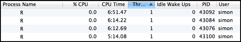
What the preceding results illustrate is that because of the variation in compute time per task, workers are left waiting for the longest task in a block to complete before they are all assigned their next task to compute. If you watch the process utilization during execution, you will see this behavior as the lightest loaded process, in particular, briefly bursts into life at the start of each of the four blocks. This scenario is particularly inefficient and can lead to significantly extended runtimes and, in the worst case, potentially no particular advantage running in parallel compared to running in serial. Notably, parLapply() avoids invoking this behavior because it first splits the available tasks into exactly cluster-sized lapply() metatasks, and clusterApply() only operates on a single block of tasks then. However, a poor balance of work across this initial split will still affect the parLapply function's overall performance.
By comparison, clusterApplyLB() distributes one task at a time per worker, and whenever a worker completes its task, it immediately hands out the next task to the first available worker. There is some extra overhead to manage this procedure due to increased communication and workers still potentially queuing to wait on their next task to be assigned if they collectively finish their previous task at the same point in time. It is only, therefore, appropriate where there is considerable variation in computation for each task, and most of the tasks take some nontrivial period of time to compute.
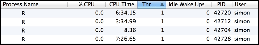
Using clusterApplyLB() in our running example leads to an improvement in overall runtime (around 10%), with significantly improved utilization across all worker processes, as follows:
> cluster <- makeCluster(4,"PSOCK")
> teval(clusterApplyLB(cluster,triples,solver))
$Duration
   user  system elapsed
  0.586   0.841 421.859
> stopCluster(cluster)
The final point to highlight here is that the a priori balancing of a distributed workload is the most efficient option when it is possible to do so. For our running example, executing the selected 16 triples in the order they are listed in with parLapply() results in the shortest overall runtime, beating clusterApplyLB() by 10 seconds and indicating that the load balancing equates to around a 3% overhead. The order of the selected triples happens to align perfectly with the parLapply function's packaging of tasks across the four-worker cluster. However, this is an artificially constructed scenario, and for the full tile-triple variable task workload, employing dynamic load balancing is the best option.
Up until now, we looked at how we can employ parallelism in the context of our own computer running R. However, our own machine can only take us so far in terms of its resources. To access the essentially unlimited compute, we need to look further afield, and to those of us mere mortals who don't have our own private data center available, we need to look to the cloud. The market leader in providing cloud services is Amazon with their AWS offering and of particular interest is their EMR service based on Hadoop that provides reliable and scalable parallel compute.
Luckily for us, there is a specific R package, segue, written by James "JD" Long and designed to simplify the whole experience of setting up an AWS EMR Hadoop cluster and utilizing it directly from an R session running on our own computer. The segue package is most applicable to run large-scale simulations or optimization problems—that is, problems that require large amounts of compute but only small amounts of data—and hence is suitable for our puzzle solver.
Before we can start to make use of segue, there are a couple of prerequisites we need to deal with: firstly, installing the segue package and its dependencies, and secondly, ensuring that we have an appropriately set-up AWS account.
Tip
Warning: credit card required!
As we work through the segue example, it is important to note that we will incur expenses. AWS is a paid service, and while there may be some free AWS service offerings that you are entitled to and the example we will run will only cost a few dollars, you need to be very aware of any ongoing billing charges you may be incurring for the various aspects of AWS that you use. It is critical that you are familiar with the AWS console and how to navigate your way around your account settings, your monthly billing statements, and, in particular, EMR, Elastic Compute Cloud (EC2), and Simple Storage
Service (S3) (these are elements as they will all be invoked when running the segue example in this chapter. For introductory information about these services, refer to the following links:
http://docs.aws.amazon.com/awsconsolehelpdocs/latest/gsg/getting-started.html
So, with our bank manager duly alerted, let's get started.
The segue package is not currently available as a CRAN package; you need to download it from the following location: https://code.google.com/p/segue/downloads/detail?name=segue_0.05.tar.gz&can=2&q=
The segue package depends on two other packages: rJava and caTools. If these are not already available within your R environment, you can install them directly from CRAN. In RStudio, this can simply be done from the Packages tab by clicking on the Install button. This will present you with a popup into which you can type the names rJava and caTools to install.
Once you download segue, you can install it in a similar manner in RStudio; the Install Packages popup has an option by which you can switch from Repository (CRAN, CRANextra) to Package Archive File and can then browse to the location of your downloaded segue package and install it. Simply loading the segue library in R will then load its dependencies as follows:
> library(segue)
Loading required package: rJava
Loading required package: caTools
Segue did not find your AWS credentials. Please run the setCredentials() function.
The segue package interacts with AWS via its secure API, and this, in turn, is only accessible through your own unique AWS credentials—that is, your AWS Access Key ID and Secret Access Key. This pair of keys must be supplied to segue through its setCredentials() function. In the next section, we will take a look at how to set up your AWS account in order to obtain your root API keys.
Our assumption at this point is that you have successfully signed up for an AWS account at http://aws.amazon.com, having provided your credit card details and so on and gone through the e-mail verification procedure. If so, then the next step is to obtain your AWS security credentials. When you are logged into the AWS console, click on your name (in the upper-right corner of the screen) and select Security Credentials from the drop-down menu.
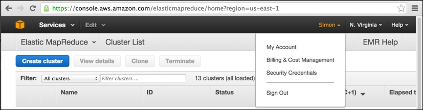
In the preceding screenshot, you can note that I have logged into the AWS console (accessible at the web URL https://console.aws.amazon.com) and have previously browsed to my EMR clusters (accessed via the Services drop-down menu to the upper-left) within the Amazon US-East-1 region in North Virginia.
This is the Amazon data center region used by segue to launch its EMR clusters. Having selected Security Credentials from your account name's drop-down menu, you will be taken to the following page:

On this page, simply expand the Access Keys tab (click on +) and then click on the revealed Create New Access Key button (note that this button will not be enabled if you already have two existing sets of security keys still active). This will present you with the following popup with new keys created, which you should immediately download and keep safe:

Let's have a look at a tip:
Tip
Warning: Keep your credentials secure at all times!
You must keep your AWS access keys secure at all times. If at any point you think that these keys may have become known to someone, you should immediately log in to your AWS account, access this page, and disable your keys. It is a simple process to create a new key pair, and in any case, Amazon's recommended security practice is to periodically reset your keys. It hopefully goes without saying that you should keep the R script where you make a call to the segue package setCredentials() particularly secure within your own computer.
The basic operation of segue follows a similar pattern and has similar names to the parallel package's cluster functions we looked at in the previous section, namely:
> setCredentials("<Access Key ID>","<Secret Access Key>")
> cluster <- createCluster(numInstances=<number of EC2 nodes>)
> results <- emrlapply(cluster, tasks, FUN,
taskTimeout=<10 mins default>)
> stopCluster(cluster) ## Remember to save your bank balance!
A key thing to note is that as soon as the cluster is created, Amazon will charge you in dollars until you successfully call stopCluster(), even if you never actually invoke the emrlapply() parallel compute function.
The createCluster() function has a large number of options (detailed in the following table), but our main focus is the numInstances option as this determines the degree of parallelism used in the underlying EMR Hadoop cluster—that is, the number of independent EC2 compute nodes employed in the cluster. However, as we are using Hadoop as the cloud cluster framework, one of the instances in the cluster must act as the dedicated master process responsible for assigning tasks to workers and marshaling the results of the parallel MapReduce operation. Therefore, if we want to deploy a 15-way parallelism, then we would need to create a cluster with 16 instances.
Another key thing to note with emrlapply() is that you can optionally specify a task timeout option (the default is 10 minutes). The Hadoop master process will consider any task that does not deliver a result (or generate a file I/O) within the timeout period as having failed, the task execution will then be cancelled (and will not be retried by another worker), and a null result will be generated for the task and returned eventually by emrlapply(). If you have individual tasks (such as simulation runs) that you know are likely to exceed the default timeout, then you should set the timeout option to an appropriate higher value (the units are minutes). Be aware though that you do want to avoid generating an infinitely running worker process that will rapidly chew through your credit balance.
The
createCluster() function has a large number of options to select resources for use and to configure the R environment running within AWS EMR Hadoop. The following table summarizes these configuration options. Take a look at the following code:
createCluster(numInstances=2,cranPackages=NULL,
  customPackages=NULL, filesOnNodes=NULL,
  rObjectsOnNodes=NULL, enableDebugging=FALSE,
  instancesPerNode=NULL, masterInstanceType="m1.large",
  slaveInstanceType="m1.large", location="us-east-1c",
  ec2KeyName=NULL, copy.image=FALSE, otherBootstrapActions=NULL,
  sourcePackagesToInstall=NULL, masterBidPrice=NULL,
  slaveBidPrice=NULL)
returns: reference object for the remote AWS EMR Hadoop cluster
In operation, segue has to perform a considerable amount of work to start up a remotely hosted EMR cluster. This includes requesting EC2 resources and utilizing S3 storage areas for the file transfer of the startup configuration and result collection. It's useful to look at the resources that are configured by segue using the AWS API through the AWS console that operates in the web browser. Using the AWS console can be critical to sorting out any problems that occur during the provisioning and running of the cluster. Ultimately, the AWS console is the last resort for releasing resources (and therefore limiting further expense) whenever segue processes go wrong, and occasionally, this does happen for many different reasons.
The following is the AWS console view of an EMR cluster that was created by segue. It just finished the emrlapply() parallel compute phase (you can see the step it just carried out , which took 34 minutes, in the center of the screen) and is now in the Waiting state, ready for more tasks to be submitted. You can note, to the lower-left, that it has one master and 15 core workers running as m1.large instances. You can also see that segue carried out two bootstrap actions on the cluster when it was created, installing the latest version of R and ensuring that all the R packages are up to date. Bootstrap actions obviously create extra overhead in readying the cluster for compute operations:
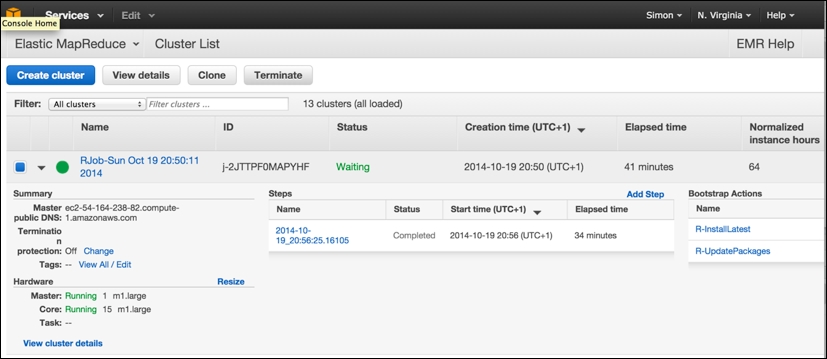
Note that it is from this screen that you can select an individual cluster and terminate it manually, freeing up the resources and preventing further charges, by clicking on the Terminate button.
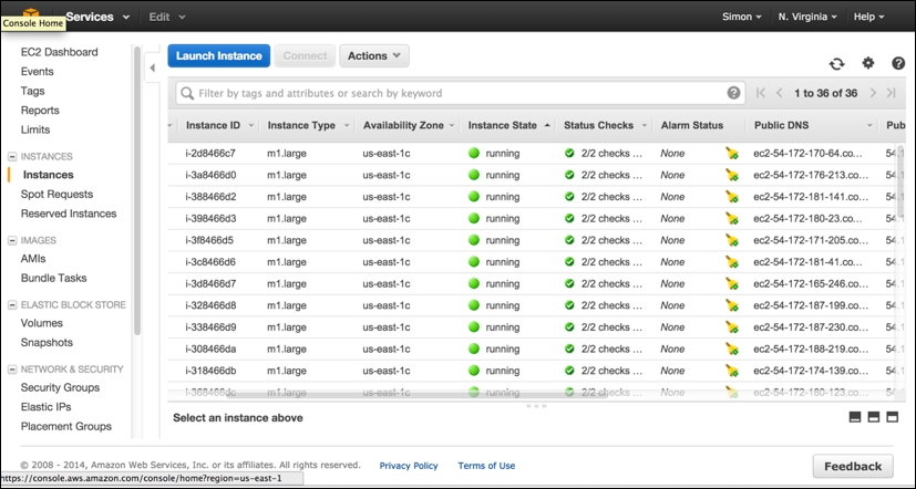
EMR resources are made up of EC2 instances, and the following view shows the equivalent view of "Hardware" in terms of the individual EC2 running instances. They are still running, clocking up AWS chargeable CPU hours, even though they are idling and waiting for more tasks to be assigned. Although EMR makes use of EC2 instances, you should never normally terminate an individual EC2 instance within the EMR cluster from this screen; you should only use the Terminate cluster operation from the main EMR Cluster List option from the preceding screen.
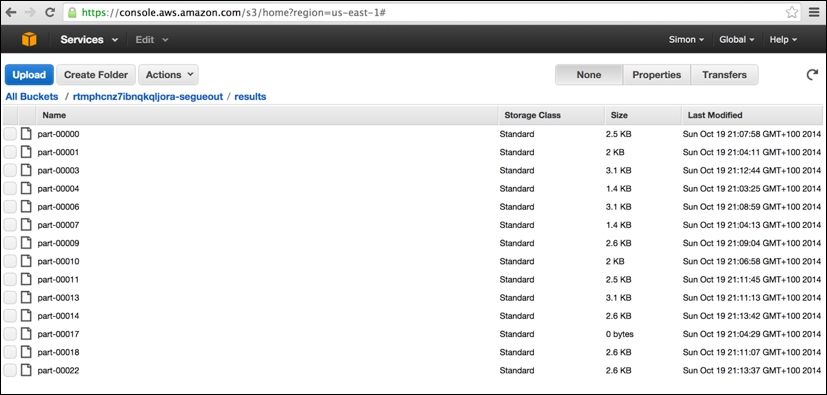
The final AWS console screen worth viewing is the S3 storage screen. The segue package creates three separate storage buckets (the name is prefixed with a unique random string), which, to all intents and purposes, can be thought of as three separate top-level directories in which various different types of files are held. These include a cluster-specific log directory (postfix: segue-logs), configuration directory (postfix: segue), and task results directory (postfix: segueout).
The following is a view of the results subdirectory within the segueout postfix folder associated with the cluster in the previous screens, showing the individual "part-XXXXX" result files being generated by the Hadoop worker nodes as they process the individual tasks:
At long last, we can now finally run our puzzle solver fully in parallel. Here, we chose to run the EMR cluster with 16 EC2 nodes, equating to one master node and 15 core worker nodes (all m1.large instances). It should be noted that there is significant overhead in both starting up the remote AWS EMR Hadoop cluster and in shutting it down again. Run the following code:
> setCredentials("<Access Key ID>","<Secret Access Key>")
>
> cluster <- createCluster(numInstances=16)
STARTING - 2014-10-19 19:25:48
## STARTING messages are repeated ~every 30 seconds until
## the cluster enters BOOTSTRAPPING phase.
STARTING - 2014-10-19 19:29:55
BOOTSTRAPPING - 2014-10-19 19:30:26
BOOTSTRAPPING - 2014-10-19 19:30:57
WAITING - 2014-10-19 19:31:28
Your Amazon EMR Hadoop Cluster is ready for action.
Remember to terminate your cluster with stopCluster().
Amazon is billing you!
## Note that the process of bringing the cluster up is complex
## and can take several minutes depending on size of cluster,
## amount of data/files/packages to be transferred/installed,
## and how busy the EC2/EMR services may be at time of request.

> results <- emrlapply(cluster, tasks, FUN, taskTimeout=10)
RUNNING - 2014-10-19 19:32:45
## RUNNING messages are repeated ~every 30 seconds until the
## cluster has completed all of the tasks.
RUNNING - 2014-10-19 20:06:46
WAITING - 2014-10-19 20:17:16

> stopCluster(cluster) ## Remember to save your bank balance!
## stopCluster does not generate any messages. If you are unable
## to run this successfully then you will need to shut the
## cluster down manually from within the AWS console (EMR).
Overall, the emrlapply() compute phase took around 34 minutes—not bad! However, the startup and shutdown phases took many minutes to run, making this aspect of overhead considerable. We could, of course, run more node instances (up to a maximum of 20 on AWS EMR currently), and we could use a more powerful instance type rather than just m1.large to speed up the compute phase further. However, such further experimentation I will leave to you, dear reader!
Tip
The AWS error in emrapply()
Very occasionally, the call to emrlapply() may fail with an error message of the following type:
Status Code: 404, AWS Service: Amazon S3, AWS Request ID: 5156824C0BE09D70, AWS Error Code: NoSuchBucket, AWS Error Message: The specified bucket does not exist…
This is a known problem with segue. The workaround is to disable your existing AWS credentials and generate a new pair of root security keys, manually terminate the AWS EMR cluster that was created by segue, restart your R session afresh, update your AWS keys in the call to setCredentials(), and then try again.
If we plot the respective elapsed time to compute the potential solution for each of the 90 starting tile-triples using R's built-in barplot() function, as can be noted in the following figure, then we will see some interesting features of the problem domain. Correct solutions found are indicated by the dark colored bars, and the rest are all fails.
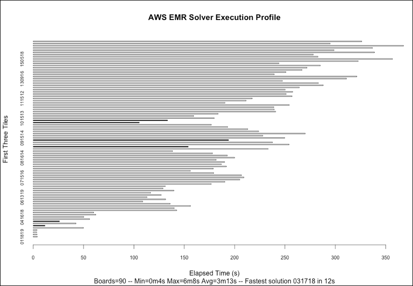
Firstly, we can note that we identified only six board-starting tile-triple configurations that result in a correct solution; I won't spoil the surprise by showing the solution here. Secondly, there is considerable variation in the time taken to explore the search space for each tile-triple with the extremes of 4 seconds and 6 minutes, with the fastest complete solution to the puzzle found in just 12 seconds. The computation is, therefore, very imbalanced, confirming what our earlier sample runs showed. There also appears to be a tendency for the time taken to increase the higher the value of the very first tile placed, something that warrants further investigation if, for example, we were keen to introduce heuristics to improve our solver's ability to choose the next best tile to place.
The cumulative computational time to solve all 90 board configurations was 4 hours and 50 minutes. In interpreting these results, we need to verify that the elapsed time is not adrift of user and system time combined. For the results obtained in this execution, there is a maximum of one percent difference in elapsed time compared to the user + system time. We would of course expect this as we are paying for dedicated resources in the AWS EMR Hadoop cluster spun up through segue.
In this chapter, you were introduced to three simple yet different techniques of utilizing parallelism in R, operating both FORK and PSOCK implemented clusters with the base R parallel package, which exploit the multicore processing capability of your own computer, and using larger-scale AWS EMR Hadoop clusters hosted remotely in the cloud directly from your computer through the segue package.
Along the way, you learned how to split a problem efficiently into independent parallelizable tasks and how imbalanced computation can be dealt with through dynamic load-balancing task management. You also saw how to effectively instrument, benchmark, and measure the runtime of your code in order to identify areas for both serial and parallel performance improvement. In fact, as an extra challenge, the current implementation of evaluateCell() can itself be improved upon and sped up….
You have also now solved Aristotle's Number Puzzle(!), and if this piqued your interest, then you can find out more about the magic hexagon at http://en.wikipedia.org/wiki/Magic_hexagon.
Who knows, you may even be able to apply your new parallel R skills to discover a new magic hexagon solution….
This chapter gave you a significant grounding in the simplest methods of parallelism using R. You should now be able to apply this knowledge directly to your own context and accelerate your own R code. In the remainder of this book, we will look at other forms of parallelism and frameworks that can be used to approach more data-intensive problems on a larger scale. You can either read the book linearly from here to the concluding one, Chapter 6, The Art of Parallel Programming, which summarizes the key learning for successful parallel programming, or you can drop into specific chapters for particular technologies, such as Chapter 2, Introduction to Message Passing, Chapter 3, Advanced Message Passing, and Chapter 4, Developing SPRINT an MPI-based R package for Supercomputers for explicit message-passing-based parallelism using MPI and Chapter 5, The Supercomputer in your Laptop for GPU-accelerated parallelism using OpenCL.
There is also a bonus chapter that will introduce you to Apache Spark, one of the newest and most popular frameworks implementing distributed parallel computation that supports complex analytics and is arguably the successor to the established, Hadoop-based Map/Reduce, which can also be applied to real-time data analysis.