Download code from GitHub
R Fundamentals for Machine Learning
You're probably used to hearing words such as big data, machine learning, and artificial intelligence in the news. It's amazing how many new applications of these terms appear every day. Recommender systems such as the ones used by Amazon, Netflix, search engines, stock market analysis, or even for speech recognition are only a few examples. Different new algorithms and new techniques emerge every year, and many of them are based on previous approaches or combine different existing algorithms. At the same time, there are more and more tutorials and courses focused on teaching them.
Many courses have a number of common limitations such as solving toy problems or focusing all of their attention on algorithms. These limitations could mean that you obtain an incorrect understanding of the data modeling approach. Thus, the modeling process entails important steps before, as business and data understanding, and data preparation. Without these previous steps, it isn't guaranteed that the model will be applied without flaws in the future. Furthermore, model development does not finish after finding an appropriate algorithm. The performance evaluation of the model, its interpretability, and the model's deployment are also very relevant and the culmination of the modeling process.
In this book, we will learn how to develop different predictive models. The applications or examples included in this book have been based on the financial sector, and will also try to create a theoretical framework that helps you understand the causes of the financial crisis, which had a dramatic impact on countries around the world.
All of the algorithms and techniques that are used in this book will be applied using the R language. Nowadays, R is one of the major languages for data science. There is an enormous debate about which language is better, R or Python. Both languages have many strengths and some weakness as well.
In my experience, R is more powerful for the analysis of financial data. I've found many R libraries that specialize in this field, but not so many in Python. Nevertheless, credit risk and financial information is very much related to the treatment of time series, which, at least in my opinion, performs better in Python. The use of recurrent or Long Short-Term Memory (LSTM) networks are better implemented in Python as well. However, R provides more powerful libraries for data visualization and interactive style. It is recommended that you use both R and Python interchangeably, depending on your project. Good resources on machine learning with Python are available at Packt, some of which are listed here for your convenience:
- Python Machine Learning – Second Edition, https://www.packtpub.com/big-data-and-business-intelligence/python-machine-learning-second-edition
- Hands-On Data Science and Python Machine Learning, https://www.packtpub.com/big-data-and-business-intelligence/hands-data-science-and-python-machine-learning
- Python Machine Learning By Example, https://www.packtpub.com/big-data-and-business-intelligence/python-machine-learning-example
In this chapter, let's revive your knowledge on machine learning and get you started with coding using R.
The following topics will be covered in this chapter:
- R and RStudio installation
- Some basics commands
- Objects, special cases, and basic operators in R
- Controlling code flow
- All about R packages
- Taking further steps
R and RStudio installation
Let's first start with installing R. It is totally free and can be downloaded from https://cloud.r-project.org/. Installing R is an easy task.
Let's look at the steps to install R on a Windows PC. For installing it on other operating systems, the steps are straightforward and are available at the same https://cloud.r-project.org/ link.
Let's start by installing R on a Windows system:
- Visit https://cloud.r-project.org/.
- Look for Download and Install R and select your operating system. We are installing for Windows, so select the Windows link.
- Go to Subdirectories and click on base.
- You will be redirected to a page that shows download R X.X.X for Windows. At the time of writing this book, Download R 3.5.2 for Windows is the version that you need to click on.
- Save and run the .exe file.
- You can now select the setup language to install R.
- A setup wizard will open and you can go on clicking Next until you reach Select Destination Location.
- Select your preferred location and click Next.
- Click the Next button several more times until R starts to install.
- After the installation is complete, R will notify you with the message Completing the R for Windows 3.5.2 Setup Wizard. You can now click on Finish.
- You can find the R shortcut on your desktop and double-click on it to start R.
- Like any other application, in case you can't find R on your desktop, you can go to the Start button, All Programs, and look for R and start it.
- You will get a screen similar to what's shown in the following screenshot:
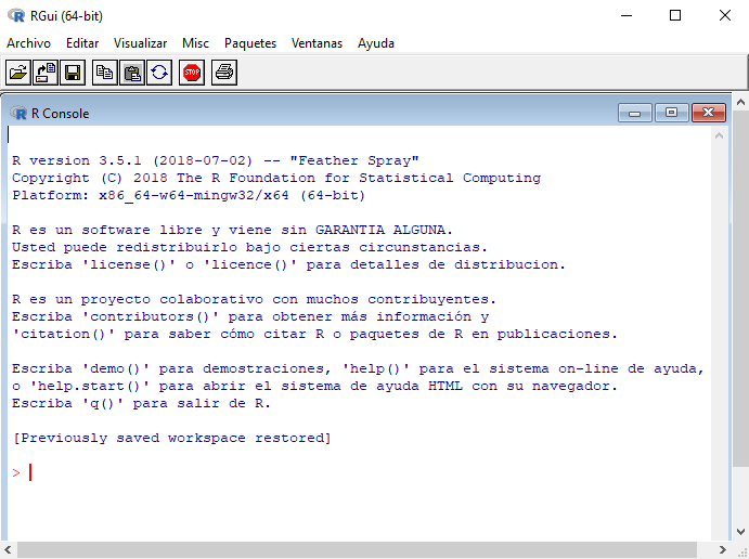
This is the R Command Prompt, waiting for input.
Things to know about R
Before moving on to typing in commands, you must know that R is a case-sensitive and interpreted language.
You can choose between manually entering commands and running a set of commands from the source file as per your will. R provides a lot of built-in functions that give most functionalities to the user. As a user, you can even create user-created functions.
You can even create and manipulate objects. You might know that objects are anything that can have an assigned value. An interactive session will require all objects to be present in the memory while the execution process is running, whereas the functions can be placed in the packages that have a reference in the current program and can be accessed as and when needed.
Using RStudio
Alongside using R, it is recommended to use RStudio. RStudio is an integrated development environment (IDE) that, like any other IDE, enhances your interaction with R.
RStudio provides you with a very well-organized interface that can clearly represent graphs, data tables, R code, and output simultaneously.
Moreover, to import and export files in different formats into R without having to write code, R offers an import wizard like feature.
Having seen the standard R GUI interface, you will see the similarities with RStudio, but the difference is that RStudio is very intuitive and user-friendly compared to the R GUI. You will have many options to choose from the menu, and you can even customize the GUI according to your requirements. RStudio for desktop is available at https://www.rstudio.com/products/rstudio/download/#download.
RStudio installation
The installation steps are very similar to the installation of R, so it isn't necessary to describe the detailed steps.
The first time you open RStudio, you will see three different windows. You can enable a fourth window by going to File, New File, and selecting R Script:

On the upper-left side window, scripts can be written and then saved and executed. The window that follows, on the left, represents the Console, where codes in R can directly be executed.
The upper-right window allows for the visualization of variables and objects that have been defined in the workspace. Furthermore, it is possible to see the history of commands that were previously executed. Finally, the bottom-right window displays the working directory.
Some basic commands
Here a list of useful commands to start with R and RStudio:
- help.start(): Starts the HTML version of R documentation
- help(command)/??command/help.search(command): Displays the help related to a specific command
- demo(): A user-friendly interface that runs some demonstrations of R scripts
- library(help=package): Lists functions and datasets in a package
- getwd(): Prints the directory that is currently active and working
- ls(): Lists the objects that are used in the current session
- setwd(mydirectory): Changes the working directory to mydirectory
- options(): Displays current settings in the options
- options(digits=5): You can print the specified digit as output
- history(): Displays previous commands until the limit of 25
- history(max.show=Inf): Displays all commands, irrespective of the limit
- savehistory(file=“myfile”): Saves the history (default file is a .Rhistory file)
- loadhistory(file=“myfile”): Recalls your command history
- save.image(): Saves the current workspace to the .RData file that's present in that particular working directory
- save(object list,file=“myfile.RData”): Saves objects into a specified file
- load(“myfile.RData”): Loads a specific object from a specified file
- q(): This will quit R for you with a prompt to save the current workspace
- library(package): Loads a library that's specific to a project
- install.package(package): Downloads and installs packages from CRAN-like repositories or even from local files
- rm(object1, object2…): Removes objects
To execute a command in RStudio, it should be written in the console, and then you must press Enter.
In RStudio, it is possible to create interactive documents by combining lines of code and plain text. R Notebooks will be helpful in interacting with R directly, and so we can have a publishing-quality document produced as output when we use it.
To create a new notebook in RStudio, go to File, New File, and R Notebook. The default notebook will open, as shown in the following screenshot:
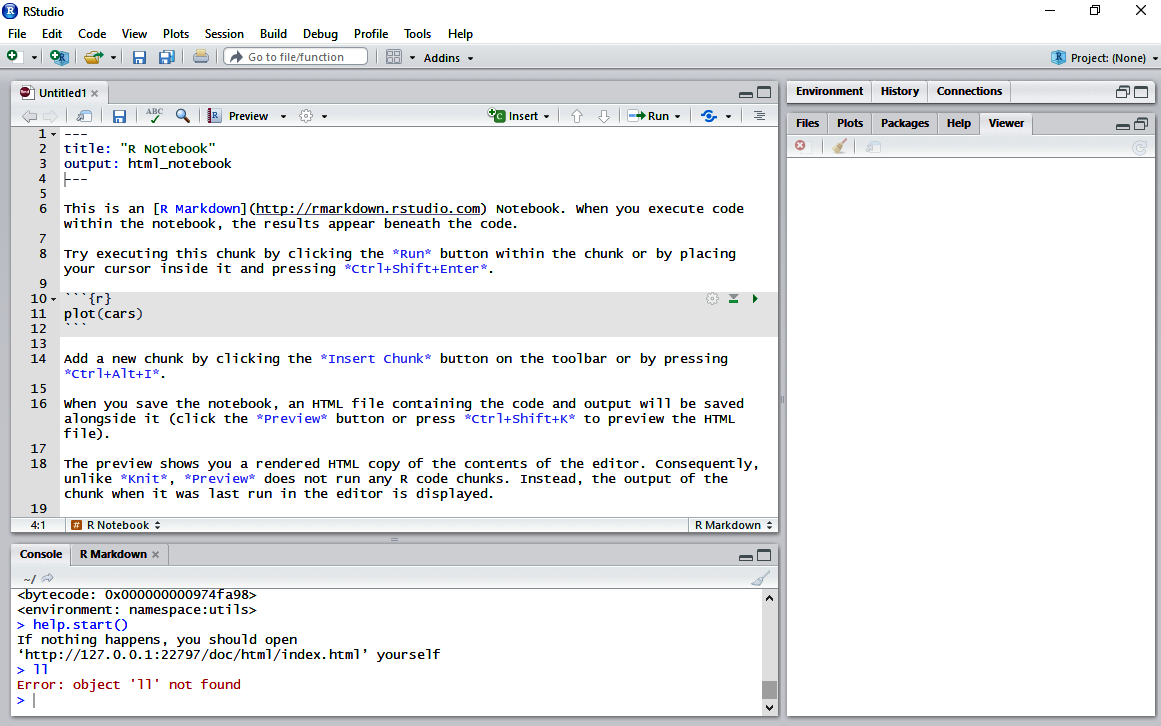
This notebook is a plain text file that has the .rmd extension. A file contains three types of content:
- An (optional) YAML header surrounded by --- lines
- R code chunks surrounded by ```r
- Text mixed with simple text formatting
R code chunks allow for the execution of code and display the results in the same notebook. To execute a chunk, click the run button within the chunk or place the cursor inside it and press Ctrl + Shift + Enter. If you wish to insert a chunk button on the toolbar, press Ctrl + Alt + I.
While saving the current notebook, a code and output file in HTML format will be generated and will be saved with the notebook. To see what the HTML file looks like, you can either click the Preview button or you can use the shortcut Ctrl + Shift + K. You can find and download all the code of this book as a R Notebook, where you can execute all the code without writing it directly.
Objects, special cases, and basic operators in R
By now, you will have figured out that R is an object-oriented language. All our variables, data, and functions will be stored in the active memory of the computer as objects. These objects can be modified using different operators or functions. An object in R has two attributes, namely, mode and length.
Mode includes the basic type of elements and has four options:
- Numeric: These are decimal numbers
- Character: Represents sequences of string values
- Complex: Combination of real and imaginary numbers, for example, x+ai
- Logical: Either true (1) or false (0)
Length means the number of elements in an object.
In most cases, we need not care whether or not the elements of a numerical object are integers, reals, or even complexes. Calculations will be carried out internally as numbers of double precision, real, or complex, depending on the case. To work with complex numbers, we must indicate explicitly the complex part.
In case an element or value is unavailable, we assign NA, a special value. Usually, operations with NA elements result in NA unless we are using some functions that can treat missing values in some way or omit them. Sometimes, calculations can lead to answers with a positive or negative infinite value (represented by R as Inf or -Inf, respectively). On the other hand, certain calculations lead to expressions that are not numbers represented by R as NaN (short for not a number).
Working with objects
You can create an object using the <- operator:
n<-10
n
## [1] 10
In the preceding code, an object called n is created. A value of 10 has been assigned to this object. The assignment can also be made using the assign() function, although this isn't very common.
Once the object has been created, it is possible to perform operations on it, like in any other programming language:
n+5
## [1] 15
These are some examples of basic operations.
Let's create our variables:
x<-4
y<-3
Now, we can carry out some basic operations:
- Sum of variables:
x + y
## [1] 7
- Subtraction of variables:
x - y
## [1] 1
- Multiplication of variables:
x * y
## [1] 12
- Division of variables:
x / y
## [1] 1.333333
- Power of variables:
x ** y
## [1] 64
Likewise in R, there are defined constants that are widely used, such as the following ones:
- The pi (
 ) number :
x * pi
## [1] 12.56637
- Exponential function:
exp(y)
## [1] 20.08554
There are also functions for working with numbers, such as the following:
- Sign (positive or negative of a number):
sign(y)
## [1] 1
- Finding the maximum value:
max(x,y)
## [1] 4
- Finding the minimum value:
min(x,y)
## [1] 3
- Factorial of a number:
factorial(y)
## [1] 6
- Square root function:
sqrt(y)
## [1] 1.732051
It is also possible to assign the result of previous operations to another object. For example, the sum of variables x and y is assigned to an object named z:
z <- x + y
z
## [1] 7
As shown previously, these functions apply if the variables are numbers, but there are also other operators to work with strings:
x > y
## [1] TRUE
x + y != 8
## [1] TRUE
The main logical operators are summarized in the following table:
| Operator | Description |
| < | Less than |
| <= | Less than or equal to |
| > | Greater than |
| >= | Greater than or equal to |
| == | Equal to |
| != | Not equal to |
| !x | Not x |
| x | y |
| x & y | x and y |
| isTRUE(x) | Test if x is TRUE |
Working with vectors
A vector is one of the basic data structures in R. It contains only similar elements, like strings and numbers, and it can have data types such as logical, double, integer, complex, character, or raw. Let's see how vectors work.
Let's create some vectors by using c():
a<-c(1,3,5,8)
a
## [1] 1 3 5 8
On mixing different objects with vector elements, there is a transformation of the elements so that they belong to the same class:
y <- c(1,3)
class(y)
## [1] "numeric"
When we apply commands and functions to a vector variable, they are also applied to every element in the vector:
y <- c(1,5,1)
y + 3
## [1] 4 8 4
You can use the : operator if you wish to create a vector of consecutive numbers:
c(1:10)
##  [1]  1  2  3  4  5  6  7  8  9 10
Do you need to create more complex vectors? Then use the seq() function. You can create vectors as complex as number of points in an interval or even to find out the step size that we might need in machine learning:
seq(1, 5, by=0.1)
##  [1] 1.0 1.1 1.2 1.3 1.4 1.5 1.6 1.7 1.8 1.9 2.0 2.1 2.2 2.3 2.4 2.5 2.6
## [18] 2.7 2.8 2.9 3.0 3.1 3.2 3.3 3.4 3.5 3.6 3.7 3.8 3.9 4.0 4.1 4.2 4.3
## [35] 4.4 4.5 4.6 4.7 4.8 4.9 5.0
seq(1, 5, length.out=22)
##  [1] 1.000000 1.190476 1.380952 1.571429 1.761905 1.952381 2.142857
##  [8] 2.333333 2.523810 2.714286 2.904762 3.095238 3.285714 3.476190
## [15] 3.666667 3.857143 4.047619 4.238095 4.428571 4.619048 4.809524
## [22] 5.000000
The rep() function is used to repeat the value of x, n number of times:
rep(3,20)
##  [1] 3 3 3 3 3 3 3 3 3 3 3 3 3 3 3 3 3 3 3 3
Vector indexing
Elements of a vector can be arranged in several haphazard ways, which can make it difficult to access them when needed. Hence, indexing makes it easier to access the elements.
You can have any type of index vectors, from logical, integer, and character.
Vector of integers starting from 1 can be used to specify elements in a vector, and it is also possible to use negative values.
Let's see some examples of indexing:
- Returns the nth element of x:
x <- c(9,8,1,5)
- Returns all x values except the nth element:
x[-3]
## [1] 9 8 5
- Returns values between a and b:
x[1:2]
## [1] 9 8
- Returns items that are greater than a and less than b:
x[x>0 & x<4]
## [1] 1
Moreover, you can even use a logical vector. In this case, either TRUE or FALSE will be returned if an element is present at that position:
x[c(TRUE, FALSE, FALSE, TRUE)]
## [1] 9 5
Functions on vectors
In addition to the functions and operators that we've seen for numerical values, there are some specific functions for vectors, such as the following:
- Sum of the elements present in a vector:
sum(x)
## [1] 23
- Product of elements in a vector:
prod(x)
## [1] 360
- Length of a vector:
length(x)
## [1] 4
- Modifying a vector using the <- operator:
x
## [1] 9 8 1 5
x[1]<-22
x
## [1] 22 8 1 5
Factor
A vector of strings of a character is known as a factor. It is used to represent categorical data, and may also include the different levels of the categorical variable. Factors are created with the factor command:
r<-c(1,4,7,9,8,1)
r<-factor(r)
r
## [1] 1 4 7 9 8 1
## Levels: 1 4 7 8 9
Factor levels
Levels are possible values that a variable can take. Suppose the original value of 1 is repeated; it will appear only once in the levels.
Factors can either be numeric or character variables, but levels of a factor can only be characters.
Let's run the level command:
levels(r)
## [1] "1" "4" "7" "8" "9"
As you can see, 1, 4, 7, 8, and 9 are the possible levels that the level r can have.
The exclude parameter allows you to exclude levels of a custom factor:
factor(r, exclude=4)
## [1] 1    <NA> 7    9    8    1
## Levels: 1 7 8 9
Finally, let's find out if our factor values are ordered or unordered:
a<- c(1,2,7,7,1,2,2,7,1,7)
a<- factor(a, levels=c(1,2,7), ordered=TRUE)
a
##  [1] 1 2 7 7 1 2 2 7 1 7
## Levels: 1 < 2 < 7
Strings
Any value that is written in single or double quotes will be considered a string:
c<-"This is our first string"
c
## [1] "This is our first string"
class(c)
## [1] "character"
String functions
Let's see how we can transform or convert strings using R.
The most relevant string examples are as follows:
- To know the number of characters in a string:
nchar(c)
## [1] 24
- To return the substring of x, originating at a particular character in x:
substring(c,4)
## [1] "s is our first string"
- To return the substring of x originating at one character located at n and ending at another character located at a place, m:
substring(c,1,4)
## [1] "This"
- To divide the string x into a list of sub chains using the delimiter as a separator:
strsplit(c, " ")
## [[1]]
## [1] "This"   "is"     "our"    "first"  "string"
- To check if the given pattern is in the string, and in that case returns true (or 1):
grep("our", c)
## [1] 1
grep("book", c)
## integer(0)
- To look for the first occurrence of a pattern in a string:
regexpr("our", c)
## [1] 9
## attr(,"match.length")
## [1] 3
## attr(,"index.type")
## [1] "chars"
## attr(,"useBytes")
## [1] TRUE
- To convert the string into lowercase:
tolower(c)
## [1] "this is our first string"
- To convert the string into capital letters:
toupper(c)
## [1] "THIS IS OUR FIRST STRING"
- To replace the first occurrence of the pattern by the given value with a string:
sub("our", "my", c)
## [1] "This is my first string"
- To replace the occurrences of the pattern with the given value with a string:
gsub("our", "my", c)
## [1] "This is my first string"
- To return the string as elements of the given array, separated by the given separator using paste(string,array, sep=“Separator”):
paste(c,"My book",sep=" : ")
## [1] "This is our first string : My book"
Matrices
You might know that a standard matrix has a two-dimensional, rectangular layout. Matrices in R are no different than a standard matrix.
Representing matrices
To represent a matrix of n elements with r rows and c columns, the matrix command is used:
m<-matrix(c(1,2,3,4,5,6), nrow=2, ncol=3)
m
##  [,1] [,2] [,3]
## [1,]    1    3    5
## [2,]    2    4    6
Creating matrices
A matrix can be created by rows instead of by columns, which is done by using the byrow parameter, as follows:
m<-matrix(c(1,2,3,4,5,6), nrow=2, ncol=3,byrow=TRUE)
m
##      [,1] [,2] [,3]
## [1,]    1    2    3
## [2,]    4    5    6
With the dimnames parameter, column names can be added to the matrix:
m<-matrix(c(1,2,3,4,5,6), nrow=2, ncol=3,byrow=TRUE,dimnames=list(c('Obs1', 'Obs2'), c('col1', 'Col2','Col3')))
m
##      col1 Col2 Col3
## Obs1    1    2    3
## Obs2    4    5    6
There are three more alternatives to creating matrices:
rbind(1:3,4:6,10:12)
##      [,1] [,2] [,3]
## [1,]    1    2    3
## [2,]    4    5    6
## [3,]   10   11   12
cbind(1:3,4:6,10:12)
##      [,1] [,2] [,3]
## [1,]    1    4   10
## [2,]    2    5   11
## [3,]    3    6   12
m<-array(c(1,2,3,4,5,6), dim=c(2,3))
m
##      [,1] [,2] [,3]
## [1,]    1    3    5
## [2,]    2    4    6
Accessing elements in a matrix
You can access the elements in a matrix in a similar way to how you accessed elements of a vector using indexing. However, the elements here would be the index number of rows and columns.
Here a some examples of accessing elements:
- If you want to access the element at a second column and first row:
m<-array(c(1,2,3,4,5,6), dim=c(2,3))
m
## [,1] [,2] [,3]
## [1,] 1 3 5
## [2,] 2 4 6
m[1,2]
## [1] 3
- Similarly, accessing the element at the second column and second row:
m[2,2]
## [1] 4
- Accessing the elements in only the second row:
m[2,]
## [1] 2 4 6
- Accessing only the first column:
m[,1]
## [1] 1 2
Matrix functions
Furthermore, there are specific functions for matrices:
- The following function extracts the diagonal as a vector:
m<-matrix(c(1,2,3,4,5,6,7,8,9), nrow=3, ncol=3)
m
##      [,1] [,2] [,3]
## [1,]    1    4    7
## [2,]    2    5    8
## [3,]    3    6    9
diag(m)
## [1] 1 5 9
- Returns the dimensions of a matrix:
dim(m)
## [1] 3 3
- Returns the sum of columns of a matrix:
colSums(m)
## [1]  6 15 24
- Returns the sum of rows of a matrix:
rowSums(m)
 ## [1] 12 15 18
- The transpose of a matrix can be obtained using the following code:
t(m)
##      [,1] [,2] [,3]
## [1,]    1    2    3
## [2,]    4    5    6
## [3,]    7    8    9
- Returns the determinant of a matrix:
det(m)
## [1] 0
- The auto-values and auto-vectors of a matrix are obtained using the following code:
eigen(m)
## eigen() decomposition
## $values
## [1]  1.611684e+01 -1.116844e+00 -5.700691e-16
##
## $vectors
##            [,1]       [,2]       [,3]
## [1,] -0.4645473 -0.8829060  0.4082483
## [2,] -0.5707955 -0.2395204 -0.8164966
## [3,] -0.6770438  0.4038651  0.4082483
Lists
If objects are arranged in an orderly manner, which makes them components, they are known as lists.
Creating lists
We can create a list using list() or by concatenating other lists:
x<- list(1:4,"book",TRUE, 1+4i)
x
## [[1]]
## [1] 1 2 3 4
##
## [[2]]
## [1] "book"
##
## [[3]]
## [1] TRUE
##
## [[4]]
## [1] 1+4i
Components will always be referred to by their referring numbers as they are ordered and numbered.
Accessing components and elements in a list
To access each component in a list, a double bracket should be used:
x[[1]]
## [1] 1 2 3 4
However, it is possible to access each element of a list as well:
x[[1]][2:4]
## [1] 2 3 4
Data frames
Data frames are special lists that can also store tabular values. However, there is a constraint on the length of elements in the lists: they all have to be of a similar length. You can consider every element in the list as columns, and their lengths can be considered as rows.
Just like lists, a data frame can have objects belonging to different classes in a column; this was not allowed in matrices.
Let's quickly create a data frame using the data.frame() function:
a <- c(1, 3, 5)
b <- c("red", "yellow", "blue")
c <- c(TRUE, FALSE, TRUE)
df <- data.frame(a, b, c)
df
##   a      b     c
##   1    red  TRUE
##   3 yellow FALSE
##   5   blue  TRUE
You can see the headers of a table as a, b, and c; they are the column names. Every line of the table represents a row, starting with the name of each row.
Accessing elements in data frames
It is possible to access each cell in the table.
To do this, you should specify the coordinates of the desired cell. Coordinates begin within the position of the row and end with the position of the column:
df[2,1]
## [1] 3
We can even use the row and column names instead of numeric values:
df[,"a"]
## [1] 1 3 5
Some packages contain datasets that can be loaded to the workspace, for example, the iris dataset:
data(iris)
Functions of data frames
Some functions can be used on data frames:
- To find out the number of columns in a data frame:
ncol(iris)
## [1] 5
- To obtain the number of rows:
nrow(iris)
## [1] 150
- To print the first 10 rows of data:
head(iris,10)
##    Sepal.Length Sepal.Width Petal.Length Petal.Width Species
## 1           5.1         3.5          1.4         0.2  setosa
## 2           4.9         3.0          1.4         0.2  setosa
## 3           4.7         3.2          1.3         0.2  setosa
## 4           4.6         3.1          1.5         0.2  setosa
## 5           5.0         3.6          1.4         0.2  setosa
## 6           5.4         3.9          1.7         0.4  setosa
## 7           4.6         3.4          1.4         0.3  setosa
## 8           5.0         3.4          1.5         0.2  setosa
## 9           4.4         2.9          1.4         0.2  setosa
## 10          4.9         3.1          1.5         0.1  setosa
- Print the last 5 rows of the iris dataset:
tail(iris,5)
##     Sepal.Length Sepal.Width Petal.Length Petal.Width   Species
## 146          6.7         3.0          5.2         2.3 virginica
## 147          6.3         2.5          5.0         1.9 virginica
## 148          6.5         3.0          5.2         2.0 virginica
## 149          6.2         3.4          5.4         2.3 virginica
## 150          5.9         3.0          5.1         1.8 virginica
- Finally, general information of the entire dataset is obtained using str():
str(iris)
## 'data.frame':    150 obs. of  5 variables:
##  $ Sepal.Length: num  5.1 4.9 4.7 4.6 5 5.4 4.6 5 4.4 4.9 ...
##  $ Sepal.Width : num  3.5 3 3.2 3.1 3.6 3.9 3.4 3.4 2.9 3.1 ...
##  $ Petal.Length: num  1.4 1.4 1.3 1.5 1.4 1.7 1.4 1.5 1.4 1.5 ...
##  $ Petal.Width : num  0.2 0.2 0.2 0.2 0.2 0.4 0.3 0.2 0.2 0.1 ...
##  $ Species     : Factor w/ 3 levels "setosa","versicolor",..: 1 1 1 1 1 1 1 1 1 1 ...
Although there are a lot of operations to work with data frames, such as merging, combining, or slicing, we won't go any deeper for now. We will be using data frames in further chapters, and shall cover more operations later.
Importing or exporting data
In R, there are several functions for reading and writing data from many sources and formats. Importing data into R is quite simple.
The most common files to import into R are Excel or text files. Nevertheless, in R, it is also possible to read files in SPSS, SYSTAT, or SAS formats, among others.
In the case of Stata and SYSTAT files, I would recommend the use of the foreign package.
Let's install and load the foreign package:
install.packages("foreign")
library(foreign)
We can use the Hmisc package for SPSS, and SAS for ease and functionality:
install.packages("Hmisc")
library(Hmisc)
Let's see some examples of importing data:
- Import a comma delimited text file. The first rows will have the variable names, and the comma is used as a separator:
mydata<-read.table("c:/mydata.csv", header=TRUE,sep=",", row.names="id")
- To read an Excel file, you can either simply export it to a comma delimited file and then import it or use the xlsx package. Make sure that the first row comprises column names that are nothing but variables.
- Let's read an Excel worksheet from a workbook, myexcel.xlsx:
library(xlsx)
mydata<-read.xlsx("c:/myexcel.xlsx", 1)
- Now, we will read a concrete Excel sheet in an Excel file:
mydata<-read.xlsx("c:/myexcel.xlsx", sheetName= "mysheet")
- Reading from the systat format:
library(foreign)
mydata<-read.systat("c:/mydata.dta")
- Reading from the SPSS format:
- First, the file should be saved from SPSS in a transport format:
getfile=’c:/mydata.sav’ exportoutfile=’c:/mydata.por’
-
- Then, the file can be imported into R with the Hmisc package:
library(Hmisc)
mydata<-spss.get("c:/mydata.por", use.value.labels=TRUE)
- To import a file from SAS, again, the dataset should be converted in SAS:
libname out xport ‘c:/mydata.xpt’; data out.mydata; set sasuser.mydata; run;
library(Hmisc)
mydata<-sasxport.get("c:/mydata.xpt")
- Reading from the Stata format:
library(foreign)
mydata<-read.dta("c:/mydata.dta")
Hence, we have seen how easy it is to read data from different file formats. Let's see how simple exporting data is.
There are analogous functions to export data from R to other formats. For SAS, SPSS, and Stata, the foreign package can be used. For Excel, you will need the xlsx package.
Here are a few exporting examples:
- We can export data to a tab delimited text file like this:
write.table(mydata, "c:/mydata.txt", sep="\t")
- We can export to an Excel spreadsheet like this:
library(xlsx)
write.xlsx(mydata, "c:/mydata.xlsx")
- We can export to SPSS like this:
library(foreign)
write.foreign(mydata, "c:/mydata.txt", "c:/mydata.sps",   package="SPSS")
- We can export to SAS like this:
library(foreign)
write.foreign(mydata, "c:/mydata.txt", "c:/mydata.sas",   package="SAS")
- We can export to Stata like this:
library(foreign)
write.dta(mydata, "c:/mydata.dta")
Working with functions
Functions are the core of R, and they are useful to structure and modularize code. We have already seen some functions in the preceding section. These functions can be considered built-in functions that are available on the basis of R or where we install some packages.
On the other hand, we can define and create our own functions based on different operations and computations we want to perform on the data. We will create functions in R using the function() directive, and these functions will be stored as objects in R.
Here is what the structure of a function in R looks like:
myfunction <- function(arg1, arg2, … )
{
statements
return(object)
}
The objects specified under a function as local to that function and the resulting objects can have any data type. We can even pass these functions as arguments for other functions.
Functions in R support nesting, which means that we can define a function within a function and the code will work just fine.
The resulting value of a function is known as the last expression evaluated on execution.
Once a function is defined, we can use that function using its name and passing the required arguments.
Let's create a function named squaredNum, which calculates the square value of a number:
squaredNum<-function(number)
 {
   a<-number^2
   return(a)
 }
Now, we can calculate the square of any number using the function that we just created:
squaredNum(425)
 ## [1] 180625
As we move on in this book, we will see how important such user-defined functions are.
Controlling code flow
R has a set of control structures that organize the flow of execution of a program, depending on the conditions of the environment. Here are the most important ones:
- If/else: This can test a condition and execute it accordingly
- for: Executes a loop that repeats for a certain number of times, as defined in the code
- while: This evaluates a condition and executes only until the condition is true
- repeat: Executes a loop an infinite number of times
- break: Used to interrupt the execution of a loop
- next: Used to jump through similar iterations to decrease the number of iterations and time taken to get the output from the loop
- return: Abandons a function
The structure of if else is as if (test_expression) { statement }.
Here, if the test_expression returns true, the statement will execute; otherwise, it won't.
An additional else condition can be added like if (test_expression) { statement1 } else { statement2 }.
In this case, the else condition is executed only if test_expression returns false.
Let's see how this works. We will evaluate an if expression like so:
x<-4
y<-3
if (x >3) {
 y <- 10
} else {
  y<- 0
}
Since x takes a value higher than 3, then the y value should be modified to take a value of 10:
print(y)
## [1] 10
If there are more than two if statements, the else expression is transformed into else if like this if ( test_expression1) { statement1 } else if ( test_expression2) { statement2 } else if ( test_expression3) { statement3 } else { statement4 }.
The for command takes an iterator variable and assigns its successive values of a sequence or vector. It is usually used to iterate on the elements of an object, such as vector lists.
An easy example is as follows, where the i variable takes different values from 1 to 10 and prints them. Then, the loop finishes:
for (i in 1:10){
 print(i)
}
## [1] 1
## [1] 2
## [1] 3
## [1] 4
## [1] 5
## [1] 6
## [1] 7
## [1] 8
## [1] 9
## [1] 10
Additionally, loops can be nested in the same code:
x<- matrix(1:6,2,3)

for (i in seq_len(nrow(x))){
  for (j in seq_len(ncol(x))){
     print(x[i,j])}
}
## [1] 1
## [1] 3
## [1] 5
## [1] 2
## [1] 4
## [1] 6
The while command is used to create loops until a specific condition is met. Let's look at an example:
x <- 1

 while (x >= 1 & x < 20){
  print(x)
  x = x+1
  }
## [1] 1
## [1] 2
## [1] 3
## [1] 4
## [1] 5
## [1] 6
## [1] 7
## [1] 8
## [1] 9
## [1] 10
## [1] 11
## [1] 12
## [1] 13
## [1] 14
## [1] 15
## [1] 16
## [1] 17
## [1] 18
## [1] 19
Here, values of x are printed, while x takes higher values than 1 and less than 20. While loops start by testing the value of a condition, if true, the body of the loop is executed. After it has been executed, it will test the condition again, and keep on testing it until the result is false.
The repeat and break commands are related. The repeat command starts an infinite loop, so the only way out of it is through the break instruction:
x <- 1
repeat{
  print(x)
  x = x+1
  if (x == 6){
     break
     }
  }
## [1] 1
## [1] 2
## [1] 3
## [1] 4
## [1] 5
We can use the break statement inside for and while loops to stop the iterations of the loop and control the flow.
Finally, the next command can be used to skip some iterations without getting them terminated. When the R parser reads next, it terminates the current iteration and moves on to another new iteration.
Let's look at an example of next, where 20 iterations are skipped:
for (i in 1:15){
      if (i <= 5){
      next
      } else { print(i)
} }
## [1] 6
## [1] 7
## [1] 8
## [1] 9
## [1] 10
## [1] 11
## [1] 12
## [1] 13
## [1] 14
## [1] 15
Before we start the next chapters of this book, it is recommended to practice these codes. Take your time and think about the code and how to use it. In the upcoming chapters, you will see a lot of code and new functions. Don't be concerned if you don't understand all of them. It is more important to have an understanding of the entire process to develop a predictive model and all the things you can do with R.
I have tried to make all of the code accessible, and it is possible to replicate all the tables and results provided in this book. Just enjoy understanding the process and reuse all the code you need in your own applications.
All about R packages
Packages in R are a collection of functions and datasets that are developed by the community.
Installing packages
Although R contains several functions in its basic installation, we will need to install additional packages to add new R functionalities. For example, with R it is possible to visualize data using the plot function. Nevertheless, we could install the ggplot2 package to obtain more pretty plots.
A package mainly includes R code (not always just R code), documentation with explanations about the package and functions inside it, examples, and even datasets.
Packages are placed on different repositories where you can install them.
Two of the most popular repositories for R packages are as follows:
- CRAN: The official repository, maintained by the R community around the world. All of the packages that are published on this repository should meet quality standards.
- GitHub: This repository is not specific for R packages, but many of the packages have open source projects located in them. Unlike CRAN, there is no review process when a package is published.
To install a package from CRAN, use the install.packages() command. For example, the ggplot2 package can be installed using the following command:
install.packages("ggplot2")
To install packages from repositories other than CRAN, I would recommend using the devtools package:
install.packages("devtools")
This package simplifies the process of installing packages from different repositories. With this package, some functions are available, depending on the repository you want to download a package from.
For example, use install_cran to download a package from CRAN or install_github() to download it from GitHub.
After the package has been downloaded and installed, we'll load it into our current R session using the library function. It is important to load packages so that we can use these new functions in our R session:
library(ggplot2)
The require function can be used to load a package. The only difference between require and library is that, in case the specific package is not found, library will show an error, but require will continue the execution of code without showing any error.
Necessary packages
To run all the code that's presented in this book, you need to install some of the packages we have mentioned. Specifically, you need to install the following packages (alphabetically ordered):
- Amelia: Package for missing data visualization and imputation.
- Boruta: Implements a feature selection algorithm for finding relevant variables.
- caret: This package (short for classification and regression training) implements several machine learning algorithms for building predictive models.
- caTools: Contains several basic utility functions, including predictive metrics or functions to split samples.
- choroplethr/choroplethrMaps: Creates maps in R.
- corrplot: Calculates correlation among variables and displays them graphically.
- DataExplorer: Includes different functions for data exploration process.
- dplyr: Package for data manipulation.
- fBasics: Includes techniques of explorative data analysis.
- funModeling: Functions for data cleaning, importance variable analysis, and model performance.
- ggfortify: Functions for data visualization tools for statistical analysis.
- ggplot2: System for declaratively creating graphics.
- glmnet: A package oriented toward Lasso and elastic-net regularized regression models.
- googleVis: R interface to Google Charts.
- h2o: A package that includes fast and scalable algorithms, including gradient boosting, random forest, and deep learning.
- h2oEnsemble: Provides functionality to create ensembles from the base learning algorithms that are accessible via the h2o package.
- Hmisc: Contains many functions that are useful for data analysis and also for importing files from different formats.
- kohonen: Facilitates the creation and visualization of self-organizing maps.
- lattice: A package to create powerful graphs.
- lubridate: Incorporates functions to work with dates in an easy way.
- MASS: Contains several statistical functions.
- plotrix: This has many plots, labeling, axis, and color scaling functions.
- plyr: This contains tools that can split, apply, and combine data.
- randomForest: Algorithms for random forests for classification and regression.
- rattle: This provides a GUI for different R packages that can aid in data mining.
- readr: Provides a fast and friendly way to read files from .csv, .tsv, or .fwf files.
- readtext: Functions to import and handle plain and formatted text files.
- recipes: Useful package for data manipulation and analysis.
- rpart: Implements classification and regression trees.
- rpart.plot: The easiest way to plot a tree that's created using the rpart package.
- Rtsne: Implementation of t-distributed Stochastic Neighbor Embedding (t-SNE).
- RWeka: RWeka has many algorithms for data mining and also tools that can pre-process and classify data. It provides an easy interface to perform operations like regression, clustering, association, and visualization.
- rworldmap: Enables mapping of country-level and gridded user datasets.
- scales: This provides methods that can automatically detect breaks, determine labels for axes, and legends. It does the work of mapping.
- smbinning: A set of functions to build scoring models.
- SnowballC: This can easily implement the very famous Porter's word stemming algorithm that collapses words into root nodes and compares the vocabulary.
- sqldf: Functions to manipulate R data frames using SQL.
- tibbletime: Useful functions to work with time series.
- tidyquant: A package focused on retrieving, manipulating, and scaling financial data analysis in the easiest way possible.
- tidyr: Includes functions for data frame manipulations.
- tidyverse: This is one package that contains packages for manipulating the data, exploring, and visualizing.
- tm: Package for text mining in R.
- VIM: Using this package, missing packages can be visualized.
- wbstats: This gives you access to data and statistics from the World Bank API.
- WDI: Search, extract, and format data from the World Bank's World Development Indicators (WDI).
- wordcloud: This package gives you the powerful functions that can help you in creating pretty word clouds. It can also help in visualizing the differences and similarities between two documents.
Once these packages have been installed, we can start working with all the code that's contained in the following chapters.
Taking further steps
We will be using the US bankruptcy problem statement to help you understand machine learning processes in depth and also to give you hands-on experience in dealing with and solving real-world problems. All the following chapters will describe each step in detail.
The objective of the following chapters is to describe all the steps and alternatives to develop a model based on machine learning techniques.
We will see several steps, starting from the extraction of the information and the generation of new variables up to the validation of the model. As we will see, in each step of the development, some alternatives or multiple steps are possible. In most of the cases, the best alternative will be the one that gives a better predictive model, but sometimes other alternatives will be chosen owing to some restrictions that are imposed by the future use of the model or the kind of problem we want to solve.
Background on the financial crisis
In this book, we will solve two different problems related to the financial crisis: the bankruptcy of the US banks and the assessment of the solvency of the European countries. Why have I chosen such a specific problem for this book? Well, the first reason is my concern about the financial crisis and my aim to try to avoid future crises. On the other hand, it is an interesting problem because a high amount of data is available, making it a very appropriate problem to understand machine learning techniques.
Most of the chapters in this book will cover the development of a predictive model to detect the failures of banks. To solve this problem, we will use a large dataset that collects some of the more typical problems you can find when dealing with different algorithms. For example, a high amount of observations and variables and an unbalanced sample means one of the categories in the classification model is much larger than the other.
Some of the steps we will see during the following chapters are as follows:
- Data collection
- Features generation
- Descriptive analysis
- Treatment of missing information
- Univariate analysis
- Multivariate analysis
- Model selection
The last chapter will focus on the development of models to detect economic imbalances in the European countries, while covering some basic text mining and clustering techniques.
Although this book is technical, one of the most important aspects of each big data and machine learning solution is understanding the problem that we need to solve.
By the end of this book, you will see that just knowing algorithms is not enough to develop models. There are many important steps that you will need to follow before jumping into running algorithms. If you pay attention to these preliminary steps, you are more likely to get good results.
In this sense, and because I'm passionate about economic theory, you can find a summary about the causes of the problems that we will solve in this book, from an economic point of view, in the repository where the code for this book is located. Specifically, the causes of the financial crisis and the contagion and transformation to a sovereign crisis are described.
Summary
In this opening chapter, we established the purpose of this book. Now that you are clear on the basics of R and its concepts, we will move on to develop two main predictive models. We will cover all the necessary steps: data collection, data analysis, and feature selection, and different algorithms will be described in a practical manner.
In the next chapter, we will start solving programming and collect the necessary data to start modeling development.