Machine Learning for Finance

This book is not only about investing or trading in the finance sector; it's much more as a direct result of the love story between computers and finance. Investment firms have customers, often insurance firms or pension funds, and these firms are financial services companies themselves and, in turn, also have customers, everyday people that have a pension or are insured.

Most bank customers are everyday people as well, and increasingly, the main way people are interacting with their bank, insurer, or pension is through an app on their mobile phone.

In the decades before today, retail banks relied on the fact that people would have to come into the branch, face-to-face, in order to withdraw cash or to make a transaction. While they were in the branch, their advisor could also sell them another product, such as a mortgage or insurance. Today's customers still want to buy mortgages and insurance, but they no longer have to do it in person at the branch. In today's world, banks tend to advise their clients online, whether it's through the app or their website.

This online aspect only works if the bank can understand its customers' needs from their data and provide tailor-made experiences online. Equally, from the customers, perspective, they now expect to be able to submit insurance claims from their phone and to get an instant response. In today's world, insurers need to be able to automatically assess claims and make decisions in order to fulfill their customers' demands.

This book is not about how to write trading algorithms in order to make a quick buck. It is about leveraging the art and craft of building machine learning-driven systems that are useful in the financial industry.

Building anything of value requires a lot of time and effort. Right now, the market for building valuable things, to make an analogy to economics, is highly inefficient. Applications of machine learning will transform the industry over the next few decades, and this book will provide you with a toolbox that allows you to be part of the change.

Many of the examples in this book use data outside the realm of "financial data." Stock market data is used at no time in this book, and this decision was made for three specific reasons.

Firstly, the examples that are shown demonstrate techniques that can usually easily be applied to other datasets. Therefore, datasets were chosen that demonstrate some common challenges that professionals, like yourselves, will face while also remaining computationally tractable.

Secondly, financial data is fundamentally time dependent. To make this book useful over a longer span of time, and to ensure that as machine learning becomes more prominent, this book remains a vital part of your toolkit, we have used some non-financial data so that the data discussed here will still be relevant.

Finally, using alternative and non-classical data aims to inspire you to think about what other data you could use in your processes. Could you use drone footage of plants to augment your grain price models? Could you use web browsing behavior to offer different financial products? Thinking outside of the box is a necessary skill to have if you want to make use of the data that is around you.

What do we mean by machine learning? Most computer programs today are handcrafted by humans. Software engineers carefully craft every rule that governs how software behaves and then translate it into computer code.

If you are reading this as an eBook, take a look at your screen right now. Everything that you see appears there because of some rule that a software engineer somewhere crafted. This approach has gotten us quite far, but that's not to say there are no limits to it. Sometimes, there might just be too many rules for humans to write. We might not be able to think of rules since they are too complex for even the smartest developers to come up with.

As a brief exercise, take a minute to come up with a list of rules that describe all dogs, but clearly distinguish dogs from all other animals. Fur? Well, cats have fur, too. What about a dog wearing a jacket? That is still a dog, just in a jacket. Researchers have spent years trying to craft these rules, but they've had very little success.

Humans don't seem to be able to perfectly tell why something is a dog, but they know a dog when they see a dog. As a species, we seem to detect specific, hard-to-describe patterns that, in aggregate, let us classify an animal as a dog. Machine learning attempts to do the same. Instead of handcrafting rules, we let a computer develop its own rules through pattern detection.

There are different ways this can work, and we're now going to look at three different types of learning: supervised, unsupervised, and reinforcement learning.

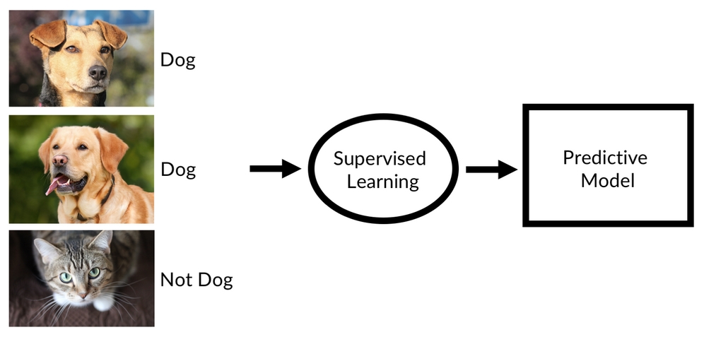
Let's go back to our dog classifier. There are in fact many such classifiers currently in use today. If you use Google images, for example, and search for "dog," it will use an image classifier to show you pictures of dogs. These classifiers are trained under a paradigm known as supervised learning.

Supervised learning

In supervised learning, we have a large number of training examples, such as images of animals, and labels that describe what the expected outcome for those training examples is. For example, the preceding figure would come with the label "dog," while an image of a cat would come with a label "not a dog."

If we have a high number of these labeled training examples, we can train a classifier on detecting the subtle statistical patterns that differentiate dogs from all other animals.

If a supervised learning classifier encounters something that's very different from the training data, it can often get confused and will just output nonsense.

While supervised learning has made great advances over the last few years, most of this book will focus on working with labeled examples. However, sometimes we may not have labels. In this case, we can still use machine learning to find hidden patterns in data.

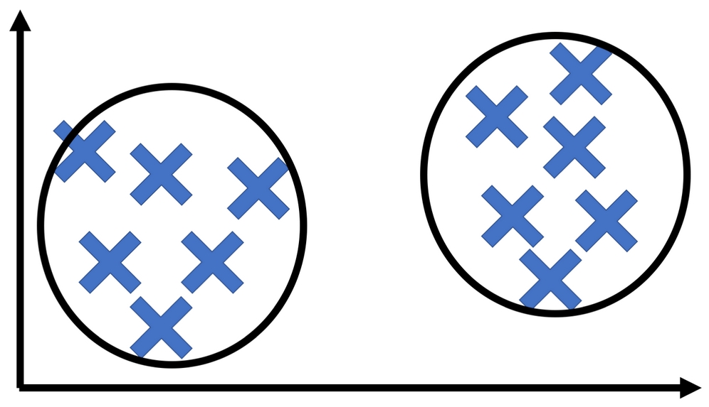
Clustering is a common form of unsupervised learning

Imagine a company that has a number of customers for its products. These customers can probably be grouped into different market segments, but what we don't know is what the different market segments are. We also cannot ask customers which market segment they belong to because they probably don't know. Which market segment of the shampoo market are you? Do you even know how shampoo firms segment their customers?

In this example, we would like an algorithm that looks at a lot of data from customers and groups them into segments. This is an example of unsupervised learning.

This area of machine learning is far less developed than supervised learning, but it still holds great potential.

In reinforcement learning, we train agents who take actions in an environment, such as a self-driving car on the road. While we do not have labels, that is, we cannot tell what the correct action is in any situation, we can assign rewards or punishments. For example, we could reward keeping a proper distance from the car in front.

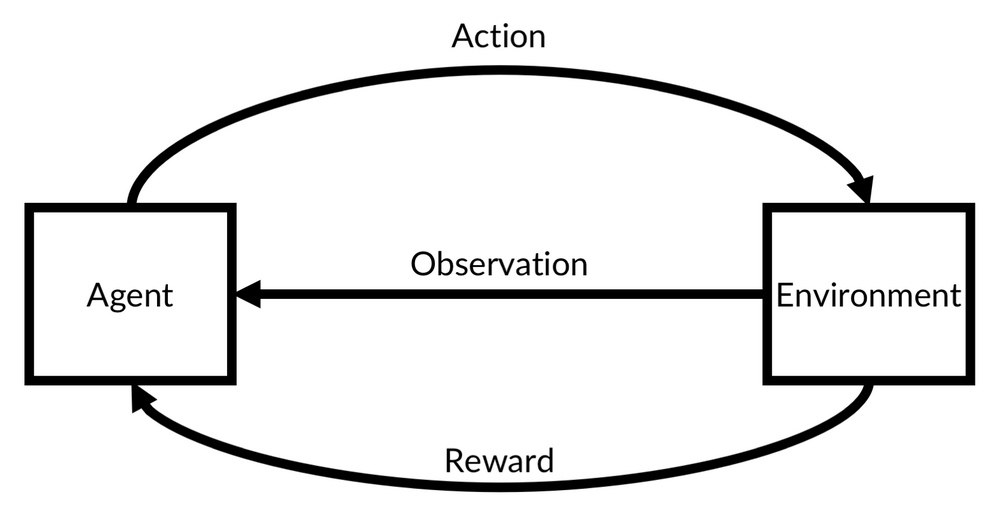
Reinforcement learning

A driving instructor does not tell the student to "push the brake halfway down while moving the steering wheel two degrees to the right," but rather they tell the student whether they are doing well or not, while the student figures out the exact amount of brakes to use.

Reinforcement learning has also made some remarkable progress in the past couple of years and is considered by many to be a promising avenue toward general artificial intelligence, that being computers that are as smart as humans.

Before we can start, you will need to set up your workspace. The examples in this book are all meant to run in a Jupyter notebook. Jupyter notebooks are an interactive development environment mostly used for data-science applications and are considered the go-to environment to build data-driven applications in.

You can run Jupyter notebooks either on your local machine, on a server in the cloud, or on a website such as Kaggle.

Deep learning is computer intensive, and the data used in the examples throughout this book are frequently over a gigabyte in size. It can be accelerated by the use of Graphics Processing Units (GPUs), which were invented for rendering video and games. If you have a GPU enabled computer, you can run the examples locally. If you do not have such a machine, it is recommended to use a service such as Kaggle kernels.

Learning deep learning used to be an expensive endeavor because GPUs are an expensive piece of hardware. While there are cheaper options available, a powerful GPU can cost up to $10,000 if you buy it and about $0.80 an hour to rent it in the cloud.

If you have many, long-running training jobs, it might be worth considering building a "deep learning" box, a desktop computer with a GPU. There are countless tutorials for this online and a decent box can be assembled for as little as a few hundred dollars all the way to $5,000.

The examples in this book can all be run on Kaggle for free, though. In fact, they have been developed using this site.

Kaggle is a popular data-science website owned by Google. It started out with competitions in which participants had to build machine learning models in order to make predictions. However, over the years, it has also had a popular forum, an online learning system and, most importantly for us, a hosted Jupyter service.

To use Kaggle, you can visit their website at https://www.kaggle.com/. In order to use the site, you will be required to create an account.

After you've created your account, you can find the Kernels page by clicking on Kernels located in the main menu, as seen in the following screenshot:

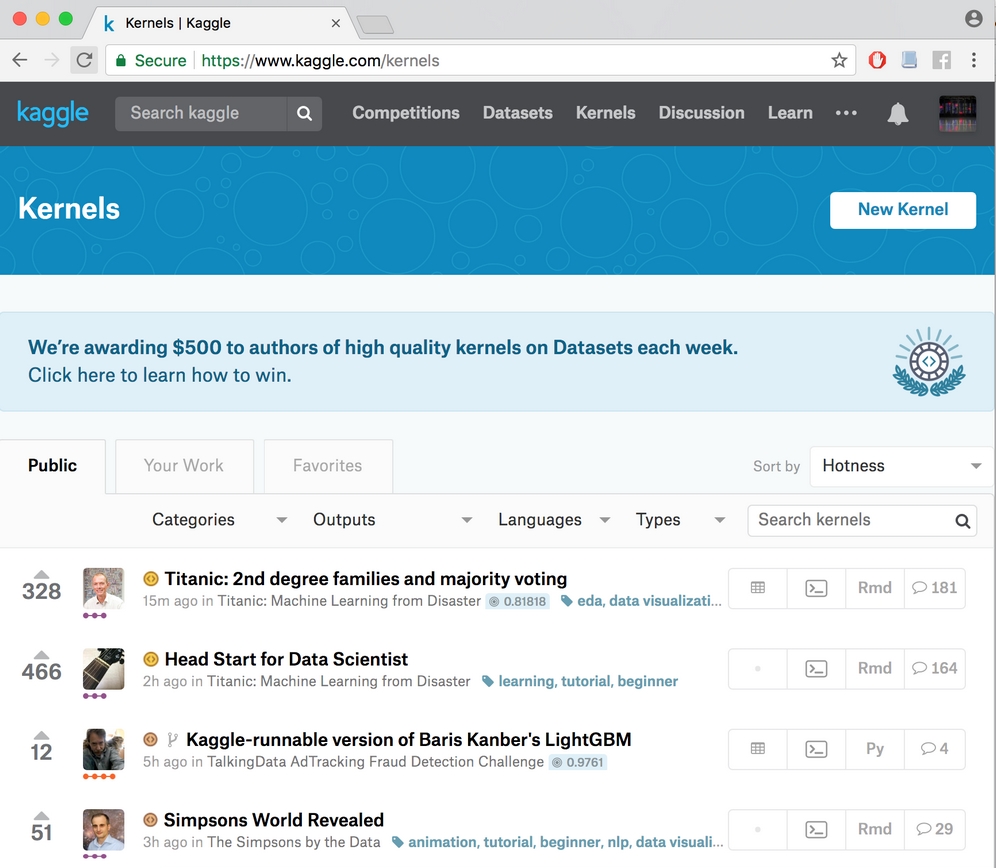
Public Kaggle kernels

In the preceding screenshot, you can see a number of kernels that other people have both written and published. Kernels can be private, but publishing kernels is a good way to show skills and share knowledge.

To start a new kernel, click New Kernel. In the dialog that follows, you want to select Notebook:

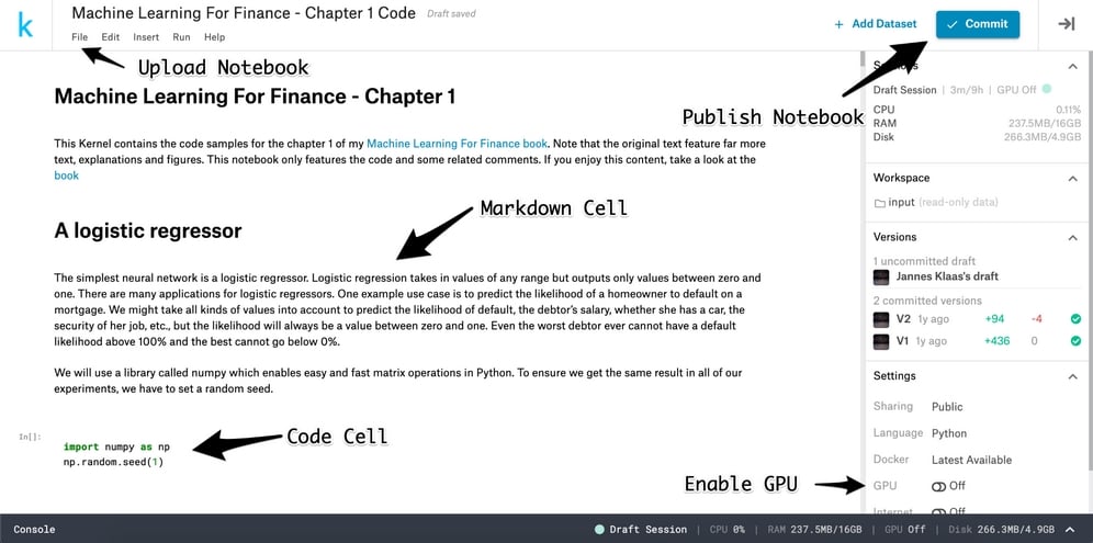
The kernel editor

You will get to the kernel editor, which looks like the preceding screenshot.

Note that Kaggle is actively iterating on the kernel design, and so a few elements might be in different positions, but the basic functionality is the same. The most important piece of a notebook is the code cells. Here you can enter the code and run it by clicking the run button on the bottom left, or alternatively by pressing Shift + Enter.

The variables you define in one cell become environment variables, so you can access them in another cell. Markdown cells allow you to write text in markdown format to add a description to what is going on in your code. You can upload and download notebooks with the little cloud buttons featured in the top-right corner.

To publish a notebook from the kernel editor, firstly you must click the Commit & Run button and then set the notebook to Public in the settings. To enable a GPU on your notebook, make sure to check the Enable GPU button located in the bottom right. It's important to remember that this will restart your notebook, so your environment variables will be lost.

Once you run the code, the run button turns into a stop button. If your code ever gets stuck, you can interrupt it by clicking that stop button. If you want to wipe all environment variables and begin anew, simply click the restart button located in the bottom-right corner.

With this system, you can connect a kernel to any dataset hosted on Kaggle, or alternatively you can just upload a new dataset on the fly. The notebooks belonging to this book already come with the data connection.

Kaggle kernels come with the most frequently used packages preinstalled, so for most of the time you do not have to worry about installing packages.

Sometimes this book does use custom packages not installed in Kaggle by default. In this case, you can add custom packages at the bottom of the Settings menu. Instructions for installing custom packages will be provided when they are used in this book.

Kaggle kernels are free to use and can save you a lot of time and money, so it's recommended to run the code samples on Kaggle. To copy a notebook, go to the link provided at the beginning of the code section of each chapter and then click Fork Notebook. Note that Kaggle kernels can run for up to six hours.

$ jupyter notebook

$ sudo pip install TensorFlow

$ sudo pip install Keras

Amazon Web Services (AWS) provides an easy-to-use, preconfigured way to run deep learning in the cloud.

Visit https://aws.amazon.com/machine-learning/amis/ for instructions on how to set up an Amazon Machine Image (AMI). While AMIs are paid, they can run longer than Kaggle kernels. So, for big projects, it might be worth using an AMI instead of a kernel.

To run the notebooks for this book on an AMI, first set up the AMI, then download the notebooks from GitHub, and then upload them to your AMI. You will have to download the data from Kaggle as well. See the Using data locally section for instructions.

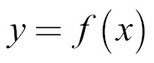
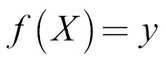
There are many views on how best to think about neural networks, but perhaps the most useful is to see them as function approximators. Functions in math relate some input, x, to some output, y. We can write it as the following formula:

A simple function could be like this:

In this case, we can give the function an input, x, and it would quadruple it:

You might have seen functions like this in school, but functions can do more; as an example, they can map an element from a set (the collection of values the function accepts) to another element of a set. These sets can be something other than simple numbers.

A function could, for example, also map an image to an identification of what is in the image:

This function would map an image of a cat to the label "cat," as we can see in the following diagram:

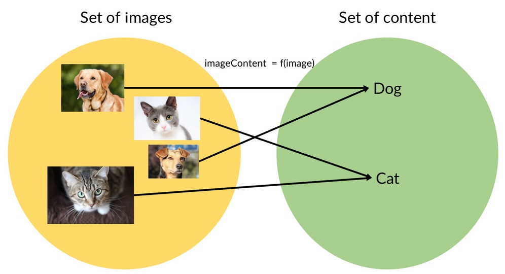
Mapping images to labels

We should note that for a computer, images are matrices full of numbers and any description of an image's content would also be stored as a matrix of numbers.

A neural network, if it is big enough, can approximate any function. It has been mathematically proven that an indefinitely large network could approximate every function. While we don't need to use an indefinitely large network, we are certainly using very large networks.

Modern deep learning architectures can have tens or even hundreds of layers and millions of parameters, so only storing the model already takes up a few gigabytes. This means that a neural network, if it's big enough, could also approximate our function, f, for mapping images to their content.

The condition that the neural network has to be "big enough" explains why deep (big) neural networks have taken off. The fact that "big enough" neural networks can approximate any function means that they are useful for a large number of tasks.

Over the course of this book, we will build powerful neural networks that are able to approximate extremely complex functions. We will be mapping text to named entities, images to their content, and even news articles to their summaries. But for now, we will work with a simple problem that can be solved with logistic regression, a popular technique used in both economics and finance.

We will be working with a simple problem. Given an input matrix, X, we want to output the first column of the matrix, X₁. In this example, we will be approaching the problem from a mathematical perspective in order to gain some intuition for what is going on.

Later on in this chapter, we will implement what we have described in Python. We already know that we need data to train a neural network, and so the data, seen here, will be our dataset for the exercise:

In the dataset, each row contains an input vector, X, and an output, y.

The data follows the formula:

The function we want to approximate is as follows:

In this case, writing down the function is relatively straightforward. However, keep in mind that in most cases it is not possible to write down the function, as functions expressed by deep neural networks can become very complex.

For this simple function, a shallow neural network with only one layer will be enough. Such shallow networks are also called logistic regressors.

As we just explained, the simplest neural network is a logistic regressor. A logistic regression takes in values of any range but only outputs values between zero and one.

There is a wide range of applications where logistic regressors are suitable. One such example is to predict the likelihood of a homeowner defaulting on a mortgage.

We might take all kinds of values into account when trying to predict the likelihood of someone defaulting on their payment, such as the debtor's salary, whether they have a car, the security of their job, and so on, but the likelihood will always be a value between zero and one. Even the worst debtor ever cannot have a default likelihood above 100%, and the best cannot go below 0%.

The following diagram shows a logistic regressor. X is our input vector; here it's shown as three components, X₁, X₂, and X₃.

W is a vector of three weights. You can imagine it as the thickness of each of the three lines. W determines how much each of the values of X goes into the next layer. b is the bias, and it can move the output of the layer up or down:

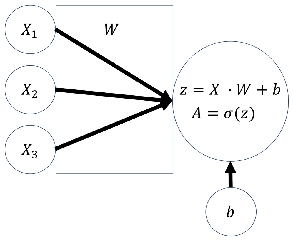
Logistic regressor

To compute the output of the regressor, we must first do a linear step. We compute the dot product of the input, X, and the weights, W. This is the same as multiplying each value of X with its weight and then taking the sum. To this number, we then add the bias, b. Afterward, we do a nonlinear step.

In the nonlinear step, we run the linear intermediate product, z, through an activation function; in this case, the sigmoid function. The sigmoid function squishes the input values to outputs between zero and one:

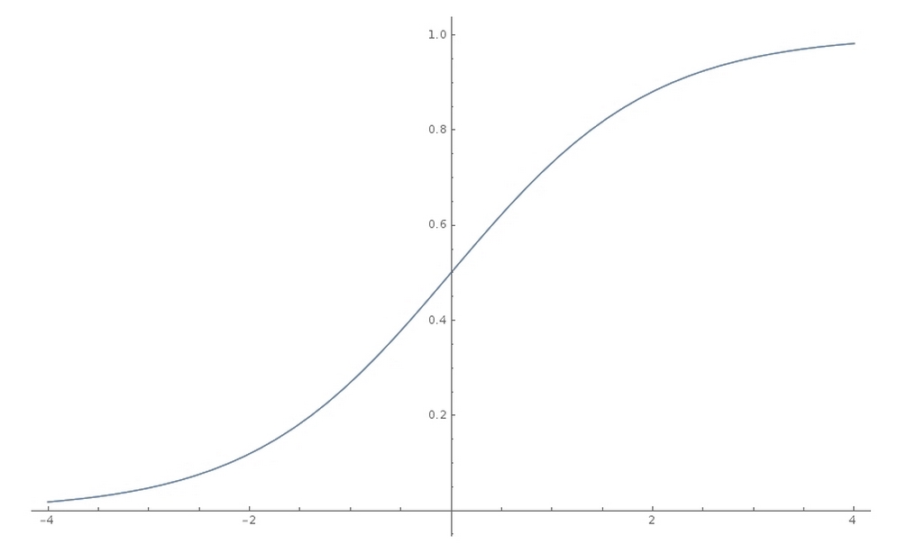
The Sigmoid function

import numpy as np
np.random.seed(1)

X = np.array([[0,1,0],
              [1,0,0],
              [1,1,1],
              [0,1,1]])

y = np.array([[0,1,1,0]]).T

def sigmoid(x):
    return 1/(1+np.exp(-x))

W = 2*np.random.random((3,1)) - 1
b = 0

z = X.dot(W) + b

A = sigmoid(z)

print(A)

out:
[[ 0.60841366]
 [ 0.45860596]
 [ 0.3262757 ]
 [ 0.36375058]]

We've already seen that we need to tweak the weights and biases, collectively called the parameters, of our model in order to arrive at a closer approximation of our desired function.

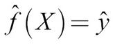
In other words, we need to look through the space of possible functions that can be represented by our model in order to find a function, , that matches our desired function, f, as closely as possible.

But how would we know how close we are? In fact, since we don't know f, we cannot directly know how close our hypothesis, , is to f. But what we can do is measure how well 's outputs match the output of f. The expected outputs of f given X are the labels, y. So, we can try to approximate f by finding a function, , whose outputs are also y given X.

We know that the following is true:

We also know that:

We can try to find f by optimizing using the following formula:

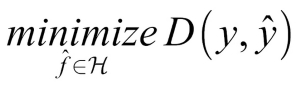
Within this formula, is the space of functions that can be represented by our model, also called the hypothesis space, while D is the distance function, which we use to evaluate how close and y are.

An example of optimizing model parameters comes from human resource management. Imagine you are trying to build a model that predicts the likelihood of a debtor defaulting on their loan, with the intention of using this to decide who should get a loan.

As training data, you can use loan decisions made by human bank managers over the years. However, this presents a problem as these managers might be biased. For instance, minorities, such as black people, have historically had a harder time getting a loan.

With that being said, if we used that training data, our function would also present that bias. You'd end up with a function mirroring or even amplifying human biases, rather than creating a function that is good at predicting who is a good debtor.

It is a commonly made mistake to believe that a neural network will find the intuitive function that we are looking for. It'll actually find the function that best fits the data with no regard for whether that is the desired function or not.

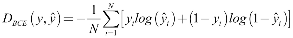
We saw earlier how we could optimize parameters by minimizing some distance function, D. This distance function, also called the loss function, is the performance measure by which we evaluate possible functions. In machine learning, a loss function measures how bad the model performs. A high loss function goes hand in hand with low accuracy, whereas if the function is low, then the model is doing well.

In this case, our issue is a binary classification problem. Because of that, we will be using the binary cross-entropy loss, as we can see in the following formula:

Let's go through this formula step by step:

In Python, this loss function is implemented as follows:

def bce_loss(y,y_hat):
  N = y.shape[0]
  loss = -1/N * (y*np.log(y_hat) + (1 - y)*np.log(1-y_hat))
  return loss

The output, A, of our logistic regressor is equal to , so we can calculate the binary cross-entropy loss as follows:

loss = bce_loss(y,A)
print(loss)

out: 
0.82232258208779863

As we can see, this is quite a high loss, so we should now look at seeing how we can improve our model. The goal here is to bring this loss to zero, or at least to get closer to zero.

You can think of losses with respect to different function hypotheses as a surface, sometimes also called the "loss surface." The loss surface is a lot like a mountain range, as we have high points on the mountain tops and low points in valleys.

Our goal is to find the absolute lowest point in the mountain range: the deepest valley, or the "global minimum." A global minimum is a point in the function hypothesis space at which the loss is at the lowest point.

A "local minimum," by contrast, is the point at which the loss is lower than in the immediately surrounding space. Local minima are problematic because while they might seem like a good function to use at face value, there are much better functions available. Keep this in mind as we now walk through gradient descent, a method for finding a minimum in our function space.

Gradient descent

Now that we know what we judge our candidate models, , by, how do we tweak the parameters to obtain better models? The most popular optimization algorithm for neural networks is called gradient descent. Within this method, we slowly move along the slope, the derivative, of the loss function.

Imagine you are in a mountain forest on a hike, and you're at a point where you've lost the track and are now in the woods trying to find the bottom of the valley. The problem here is that because there are so many trees, you cannot see the valley's bottom, only the ground under your feet.

Now ask yourself this: how would you find your way down? One sensible approach would be to follow the slope, and where the slope goes downwards, you go. This is the same approach that is taken by a gradient descent algorithm.

To bring it back to our focus, in this forest situation the loss function is the mountain, and to get to a low loss, the algorithm follows the slope, that is, the derivative, of the loss function. When we walk down the mountain, we are updating our location coordinates.

The algorithm updates the parameters of the neural network, as we are seeing in the following diagram:

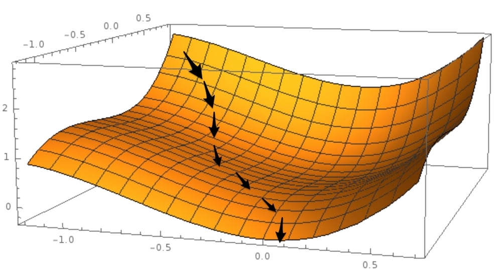
Gradient descent

Gradient descent requires that the loss function has a derivative with respect to the parameters that we want to optimize. This will work well for most supervised learning problems, but things become more difficult when we want to tackle problems for which there is no obvious derivative.

Gradient descent can also only optimize the parameters, weights, and biases of our model. What it cannot do is optimize how many layers our model has or which activation functions it should use, since there is no way to compute the gradient with respect to model topology.

These settings, which cannot be optimized by gradient descent, are called hyperparameters and are usually set by humans. You just saw how we gradually scale down the loss function, but how do we update the parameters? To this end, we're going to need another method called backpropagation.

Backpropagation

Backpropagation allows us to apply gradient descent updates to the parameters of a model. To update the parameters, we need to calculate the derivative of the loss function with respect to the weights and biases.

If you imagine the parameters of our models are like the geo-coordinates in our mountain forest analogy, calculating the loss derivative with respect to a parameter is like checking the mountain slope in the direction north to see whether you should go north or south.

The following diagram shows the forward and backward pass through a logistic regressor:

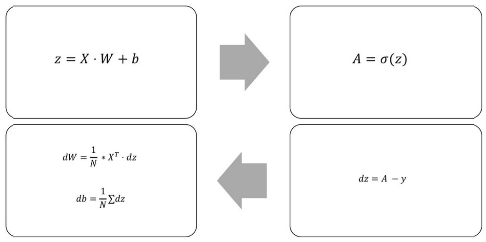
Forward and backward pass through a logistic regressor

To keep things simple, we refer to the derivative of the loss function to any variable as the d variable. For example, we'll write the derivative of the loss function with respect to the weights as dW.

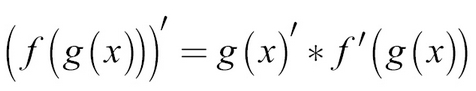
To calculate the gradient with respect to different parameters of our model, we can make use of the chain rule. You might remember the chain rule as the following:

This is also sometimes written as follows:

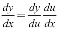
The chain rule basically says that if you want to take the derivative through a number of nested functions, you multiply the derivative of the inner function with the derivative of the outer function.

This is useful because neural networks, and our logistic regressor, are nested functions. The input goes through the linear step, a function of input, weights, and biases; and the output of the linear step, z, goes through the activation function.

So, when we compute the loss derivative with respect to weights and biases, we'll first compute the loss derivative with respect to the output of the linear step, z, and use it to compute dW. Within the code, it looks like this:

dz = (A - y)

dW = 1/N * np.dot(X.T,dz)

db = 1/N * np.sum(dz,axis=0,keepdims=True)

Parameter updates

Now we have the gradients, how do we improve our model? Going back to our mountain analogy, now that we know that the mountain goes up in the north and east directions, where do we go? To the south and west, of course!

Mathematically speaking, we go in the opposite direction to the gradient. If the gradient is positive with respect to a parameter, that is, the slope is upward, then we reduce the parameter. If it is negative, that is, downward sloping, we increase it. When our slope is steeper, we move our gradient more.

The update rule for a parameter, p, then goes like this:

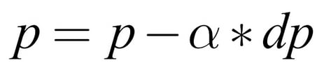
Here p is a model parameter (either in weight or a bias), dp is the loss derivative with respect to p, and is the learning rate.

The learning rate is something akin to the gas pedal within a car. It sets by how much we want to apply the gradient updates. It is one of those hyperparameters that we have to set manually, and something we will discuss in the next chapter.

Within the code, our parameter updates look like this:

alpha = 1
W -= alpha * dW
b -= alpha * db

Putting it all together

Well done! We've now looked at all the parts that are needed in order to train a neural network. Over the next few steps in this section, we will be training a one-layer neural network, which is also called a logistic regressor.

Firstly, we'll import numpy before we define the data. We can do this by running the following code:

import numpy as np
np.random.seed(1)

X = np.array([[0,1,0],
              [1,0,0],
              [1,1,1],
              [0,1,1]])

y = np.array([[0,1,1,0]]).T

The next step is for us to define the sigmoid activation function and loss function, which we can do with the following code:

def sigmoid(x):
    return 1/(1+np.exp(-x))

def bce_loss(y,y_hat):
    N = y.shape[0]
    loss = -1/N * np.sum((y*np.log(y_hat) + (1 - y)*np.log(1-y_hat)))
    return loss

We'll then randomly initialize our model, which we can achieve with the following code:

W = 2*np.random.random((3,1)) - 1
b = 0

As part of this process, we also need to set some hyperparameters. The first one is alpha, which we will just set to 1 here. Alpha is best understood as the step size. A large alpha means that while our model will train quickly, it might also overshoot the target. A small alpha, in comparison, allows gradient descent to tread more carefully and find small valleys it would otherwise shoot over.

The second one is the number of times we want to run the training process, also called the number of epochs we want to run. We can set the parameters with the following code:

alpha = 1
epochs = 20

Since it is used in the training loop, it's also useful to define the number of samples in our data. We'll also define an empty array in order to keep track of the model's losses over time. To achieve this, we simply run the following:

N = y.shape[0]
losses = []

Now we come to the main training loop:

for i in range(epochs):
    # Forward pass
    z = X.dot(W) + b 
    A = sigmoid(z)
    
    # Calculate loss
    loss = bce_loss(y,A)
    print('Epoch:',i,'Loss:',loss)
    losses.append(loss)
    
    # Calculate derivatives
    dz = (A - y)
    dW = 1/N * np.dot(X.T,dz)
    db = 1/N * np.sum(dz,axis=0,keepdims=True)    
    
    # Parameter updates
    W -= alpha * dW
    b -= alpha * db

As a result of running the previous code, we would get the following output:

out: 
Epoch: 0 Loss: 0.822322582088
Epoch: 1 Loss: 0.722897448125
Epoch: 2 Loss: 0.646837651208
Epoch: 3 Loss: 0.584116122241
Epoch: 4 Loss: 0.530908161024
Epoch: 5 Loss: 0.48523717872
Epoch: 6 Loss: 0.445747750118
Epoch: 7 Loss: 0.411391164148
Epoch: 8 Loss: 0.381326093762
Epoch: 9 Loss: 0.354869998127
Epoch: 10 Loss: 0.331466036109
Epoch: 11 Loss: 0.310657702141
Epoch: 12 Loss: 0.292068863232
Epoch: 13 Loss: 0.275387990352
Epoch: 14 Loss: 0.260355695915
Epoch: 15 Loss: 0.246754868981
Epoch: 16 Loss: 0.234402844624
Epoch: 17 Loss: 0.22314516463
Epoch: 18 Loss: 0.21285058467
Epoch: 19 Loss: 0.203407060401

You can see that over the course of the output, the loss steadily decreases, starting at 0.822322582088 and ending at 0.203407060401.

We can plot the loss to a graph in order to give us a better look at it. To do this, we can simply run the following code:

import matplotlib.pyplot as plt
plt.plot(losses)
plt.xlabel('epoch')
plt.ylabel('loss')
plt.show()

This will then output the following chart:

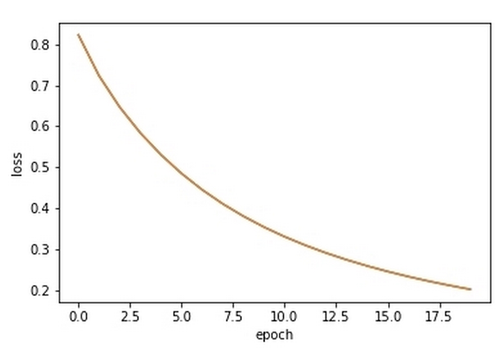
The output of the previous code, showing loss rate improving over time

We established earlier in this chapter that in order to approximate more complex functions, we need bigger and deeper networks. Creating a deeper network works by stacking layers on top of each other.

In this section, we will build a two-layer neural network like the one seen in the following diagram:

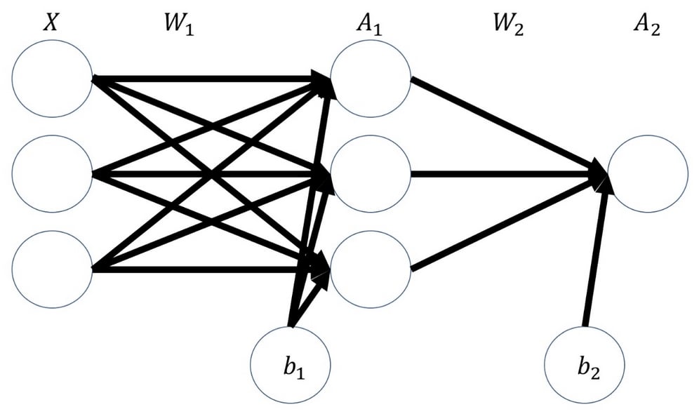
Sketch of a two-layer neural network

The input gets multiplied with the first set of weights, W₁, producing an intermediate product, z₁. This is then run through an activation function, which will produce the first layer's activations, A₁.

These activations then get multiplied with the second layer of weights, W₂, producing an intermediate product, z₂. This gets run through a second activation function, which produces the output, A₂, of our neural network:

z1 = X.dot(W1) + b1

a1 = np.tanh(z1)

z2 = a1.dot(W2) + b2

a2 = sigmoid(z2)

As you can see, the first activation function is not a sigmoid function but is actually a tanh function. Tanh is a popular activation function for hidden layers and works a lot like sigmoid, except that it squishes values in the range between -1 and 1 rather than 0 and 1:

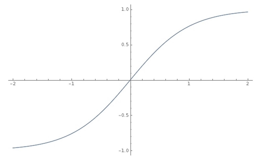
The tanh function

Backpropagation through our deeper network works by the chain rule, too. We go back through the network and multiply the derivatives:

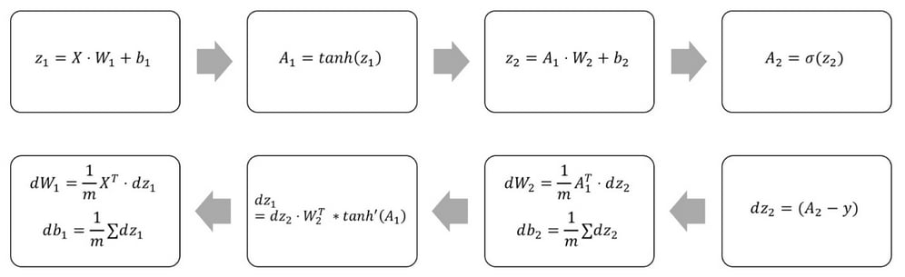
Forward and backward pass through a two-layer neural network

The preceding equations can be expressed as the following Python code:

# Calculate loss derivative with respect to the output
dz2 = bce_derivative(y=y,y_hat=a2)

# Calculate loss derivative with respect to second layer weights
dW2 = (a1.T).dot(dz2)

# Calculate loss derivative with respect to second layer bias
db2 = np.sum(dz2, axis=0, keepdims=True)

# Calculate loss derivative with respect to first layer
dz1 = dz2.dot(W2.T) * tanh_derivative(a1)

# Calculate loss derivative with respect to first layer weights
dW1 = np.dot(X.T, dz1)

# Calculate loss derivative with respect to first layer bias
db1 = np.sum(dz1, axis=0)

Note that while the size of the inputs and outputs are determined by your problem, you can freely choose the size of your hidden layer. The hidden layer is another hyperparameter you can tweak. The bigger the hidden layer size, the more complex the function you can approximate. However, the flip side of this is that the model might overfit. That is, it may develop a complex function that fits the noise but not the true relationship in the data.

Take a look at the following chart. What we see here is the two moons dataset that could be clearly separated, but right now there is a lot of noise, which makes the separation hard to see even for humans. You can find the full code for the two-layer neural network as well as for the generation of these samples in the Chapter 1 GitHub repo:

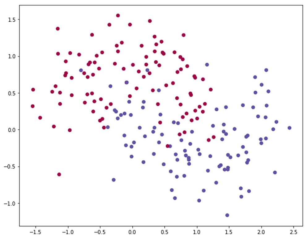
The two moons dataset

The following diagram shows a visualization of the decision boundary, that is, the line at which the model separates the two classes, using a hidden layer size of 1:

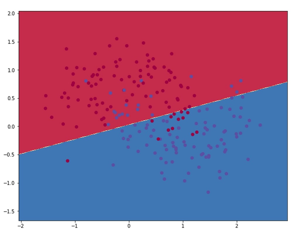
Decision boundary for hidden layer size 1

As you can see, the network does not capture the true relationship of the data. This is because it's too simplistic. In the following diagram, you will see the decision boundary for a network with a hidden layer size of 500:

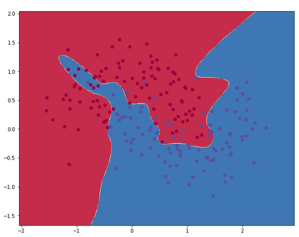
Decision boundary for hidden layer size 500

This model clearly fits the noise, but not the moons. In this case, the right hidden layer size is about 3.

Finding the right size and the right number of hidden layers is a crucial part of designing effective learning models. Building models with NumPy is a bit clumsy and can be very easy to get wrong. Luckily, there is a much faster and easier tool for building neural networks, called Keras.

Keras is a high-level neural network API that can run on top of TensorFlow, a library for dataflow programming. What this means is that it can run the operations needed for a neural network in a highly optimized way. Therefore, it's much faster and easier to use than TensorFlow. Because Keras acts as an interface to TensorFlow, it makes it easier to build even more complex neural networks. Throughout the rest of the book, we will be working with the Keras library in order to build our neural networks.

from keras.layers import Dense, Activation

from keras.models import Sequential

model = Sequential()

model.add(Dense(3,input_dim=2))

model.add(Activation('tanh'))

model.add(Dense(1))
model.add(Activation('sigmoid'))

model.summary()

out: 
Layer (type)                 Output Shape              Param #   
=================================================================
dense_3 (Dense)              (None, 3)                 9         
_________________________________________________________________
activation_3 (Activation)    (None, 3)                 0         
_________________________________________________________________
dense_4 (Dense)              (None, 1)                 4         
_________________________________________________________________
activation_4 (Activation)    (None, 1)                 0         
=================================================================
Total params: 13
Trainable params: 13
Non-trainable params: 0

model.compile(optimizer='sgd',
              loss='binary_crossentropy',
              metrics=['acc'])

history = model.fit(X,y,epochs=900)

Epoch 1/900
200/200 [==============================] - 0s 543us/step - 
loss: 0.6840 - acc: 0.5900
Epoch 2/900
200/200 [==============================] - 0s 60us/step - 
loss: 0.6757 - acc: 0.5950
...

Epoch 899/900
200/200 [==============================] - 0s 90us/step - 
loss: 0.2900 - acc: 0.8800
Epoch 900/900
200/200 [==============================] - 0s 87us/step - 
loss: 0.2901 - acc: 0.8800

from tensorflow.keras.layers import Dense, Activation

Tensors are arrays of numbers that transform based on specific rules. The simplest kind of tensor is a single number. This is also called a scalar. Scalars are sometimes referred to as rank-zero tensors.

The next tensor is a vector, also known as a rank-one tensor. The next The next ones up the order are matrices, called rank-two tensors; cube matrices, called rank-three tensors; and so on. You can see the rankings in the following table:

This book mostly uses the word tensor for rank-three or higher tensors.

TensorFlow and every other deep learning library perform calculations along a computational graph. In a computational graph, operations, such as matrix multiplication or an activation function, are nodes in a network. Tensors get passed along the edges of the graph between the different operations.

A forward pass through our simple neural network has the following graph:

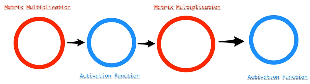
A simple computational graph

The advantage of structuring computations as a graph is that it's easier to run nodes in parallel. Through parallel computation, we do not need one very fast machine; we can also achieve fast computation with many slow computers that split up the tasks.

This is the reason why GPUs are so useful for deep learning. GPUs have many small cores, as opposed to CPUs, which only have a few fast cores. A modern CPU might only have four cores, whereas a modern GPU can have hundreds or even thousands of cores.

The entire graph of just a very simple model can look quite complex, but you can see the components of the dense layer. There is a matrix multiplication (matmul), adding bias and a ReLU activation function:

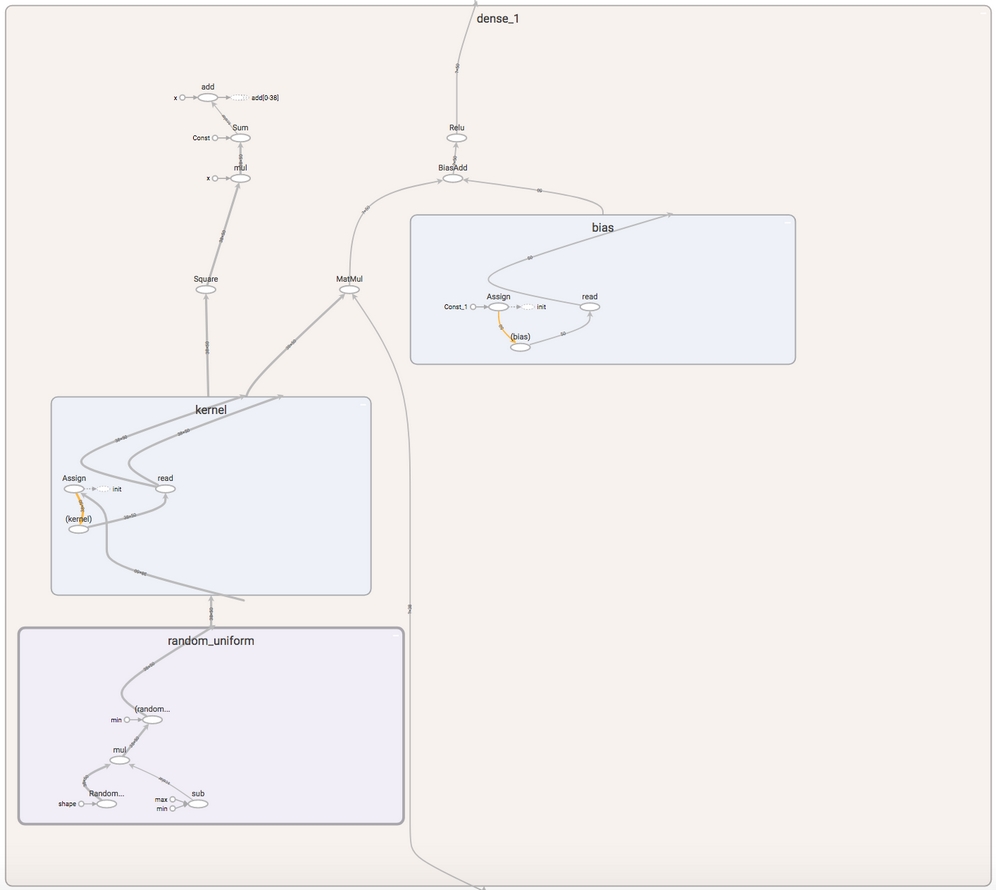
The computational graph of a single layer in TensorFlow. Screenshot from TensorBoard.

Another advantage of using computational graphs such as this is that TensorFlow and other libraries can quickly and automatically calculate derivatives along this graph. As we have explored throughout this chapter, calculating derivatives is key for training neural networks.

Now that we have finished the first chapter in this exciting journey, I've got a challenge for you! You'll find some exercises that you can do that are all themed around what we've covered in this chapter!

So, why not try to do the following:

And that's it! We've learned how neural networks work. Throughout the rest of this book, we'll look at how to build more complex neural networks that can approximate more complex functions.

As it turns out, there are a few tweaks to make to the basic structure for it to work well on specific tasks, such as image recognition. The basic ideas introduced in this chapter, however, stay the same:

The key takeaway from this chapter is that while we are looking for function f, we can try and find it by optimizing a function to perform like f on a dataset. A subtle but important distinction is that we do not know whether works like f at all. An often-cited example is a military project that tried to use deep learning to spot tanks within images. The model trained well on the dataset, but once the Pentagon wanted to try out their new tank spotting device, it failed miserably.

In the tank example, it took the Pentagon a while to figure out that in the dataset they used to develop the model, all the pictures of the tanks were taken on a cloudy day and pictures without a tank where taken on a sunny day. Instead of learning to spot tanks, the model had learned to spot grey skies instead.

This is just one example of how your model might work very differently to how you think, or even plan for it to do. Flawed data might seriously throw your model off track, sometimes without you even noticing. However, for every failure, there are plenty of success stories in deep learning. It is one of the high-impact technologies that will reshape the face of finance.

In the next chapter, we will get our hands dirty by jumping in and working with a common type of data in finance, structured tabular data. More specifically, we will tackle the problem of fraud, a problem that many financial institutions sadly have to deal with and for which modern machine learning is a handy tool. We will learn about preparing data and making predictions using Keras, scikit-learn, and XGBoost.