Learning SciPy for Numerical and Scientific Computing

The ideal programming environment for computational mathematics is one that enjoys the following characteristics: 

Among the best-known environments for numerical computations used by the scientific community, we have the powerful MATLAB® and Scilab® systems (although both of them are commercial, expensive, and do not allow any tampering with the code). Maple® and Mathematica® are more geared towards symbolic computation, although they can match many of the numerical computations from MATLAB®. As the previous two, these are also commercial, expensive, and closed to modifications. A decent alternative to MATLAB®, based on similar mathematical engine, is the GNU Octave system. Most of the MATLAB® code is easily portable in Octave. It also has the advantage of being open source. Unfortunately, the underlying programming environment is not very user friendly. It is also restricted to numerical computations.

The one environment that combines the best of all worlds is indeed the combination of Python with the NumPy and SciPy libraries. The first property that attracts the user to Python is, without a doubt, its code readability. The syntax is extremely clear and expressive. It has the advantage of supporting code written in different paradigms – object oriented, functional, or old school imperative. It allows the compilation of code for running standalone executable programs, but it can also be used interactively, or as a scripting language. This is a great advantage if the user needs to develop tools for symbolic computation. Python has been used in this sense as the basis of a firm competitor to Maple® and Mathematica®: the open-source mathematics software Sage (System for Algebra and Geometry Experimentation).

NumPy is an open-source extension to Python that adds support for multidimensional arrays of large sizes. This support allows the desired acquisition, storage, and complex manipulation of data mentioned previously. NumPy alone is a great tool to solve many numerical computations.

On top of NumPy, we have yet another open-source library, SciPy. This library contains algorithms and mathematical tools to manipulate NumPy objects, with very definite scientific and engineering objectives.

The combination of Python, NumPy, and SciPy (which henceforth should be coined "SciPy" for brevity) has been the environment of choice of many applied mathematicians for years; we work on a daily basis with both the pure mathematicians and with the hard-core engineers. One of the challenges of this trade is to bring to a single workstation the scientific production of professionals with different visions, techniques, tools, and software. SciPy is the perfect solution for coordinating everything together in a smooth, reliable, and coherent way.

Any day of the week, we are required to produce scripts in which, for example, there are combinations of experiments written and performed in SciPy itself, C/C++, Fortran, or MATLAB®. We often receive extremely large amounts of data from some signal acquisition devices. From all this heterogeneous material, we employ Python to retrieve the data, manipulate and, once finished with the analysis, produce high-quality documentation with professional-looking diagrams and visualization aids. SciPy allows performing all these tasks with ease.

This is partly because many dedicated software tools easily extend the core features of SciPy. For example, although any graphing and plotting is usually done with the Python libraries of matplotlib, there are also other packages, such as Biggles (biggles.sourceforge.net), Chaco (pypi.python.org/pypi/chaco), HippoDraw (github.com/plasmodic/hippodraw), MayaVi for 3D rendering (mayavi.sourceforge.net), or the Python Imaging Library or PIL (pythonware.com/products/pil).

Interfacing with non-Python packages is also possible. For example, the interaction of SciPy with the R statistical package can be done with RPy (rpy.sourceforge.net/rpy2.html). This allows for much more robust data analysis.

At the time when this book was written, the latest versions of Python are 2.7.3 and 3.2.3. They are both stable production releases, although the Python 2 versions are more convenient if the user needs to communicate with third-party applications. No new releases are done for Python 2, and that is why Python 3 is considered "the present and the future of Python". For the purposes of SciPy applications, we do recommend to stay with the 2.7.3 version. The language can be downloaded from the official Python site (www.python.org/download) and installed on all major systems such as Windows, Mac OS X, Linux, and Unix. It has also been ported to other platforms, including Palm OS, iOS, PlayStation, PSP, Psion, and so on. The following screenshot shows two popular options for coding in Python on an iPad – PythonMath and Sage Math. While the first application allows only the use of simple math libraries, the second permits the user to load and use both NumPy and SciPy remotely.

PythonMath and Sage Math bring Python coding to iOS devices. Sage Math allows importing NumPy and SciPy.

We shall not go into detail about the installation of Python on your system, since we already assume familiarity with this language. In case of doubt, we advise browsing the excellent book Expert Python Programming: Best practices for designing, coding, and distributing your Python software, Tarek Ziadé, Packt Publishing, where detailed explanations are given for installing any of the different implementations on different systems. It is usually a good idea to follow the directions given on the official Python website, as well. We will also assume familiarity with carrying out interactive sessions in Python, as well as writing standalone scripts.

The latest libraries for both NumPy and SciPy can be downloaded from the official SciPy site, scipy.org/Download. They both require a Python Version 2.4 or newer, so we should be in good shape at this point. We may choose to do the download from sourceforge (sourceforge.net/projects/scipy), or from Git repositories (for instance, the superpack from fonnesbeck.github.com/ScipySuperpack). It is also possible in some systems to use pre-packaged executable bundles that simplify the process. We will show here how to download and install in the most common cases.

For instance, in Mac OS X, if macports is installed, the process could not be easier. Open a terminal as superuser and, at the prompt (%), issue the following command:

% port search scipy

This presents a list of all ports that either install SciPy or use SciPy as a requirement. On that list, the one we require for Python 2.7 is the py27-scipy port. We install it (again as a superuser) by issuing the following command at prompt:

% port install py27-scipy

A few minutes later, the libraries are properly installed and ready to use. Note how macports also installs all needed requirements for us (including the NumPy libraries) without any extra effort from our part.

Under any other Unix/Linux system, if either no ports are available or if the user prefers to install from the packages downloaded from either sourceforge or Git, it is enough to perform the following steps:

Under Microsoft Windows, we recommend you install from the binary installers provided by the Enthought Python Distribution. Download and double-click!

The procedure for the installation of the SciPy libraries is exactly the same, that is, downloading and building before installing under Unix/Linux, or downloading and double-clicking under Microsoft Windows. Note that different implementations of Python might have different requirements before installing NumPy and SciPy.

SciPy is organized as a family of modules. We like to think of each module as a different field of mathematics. And as such, each has its own particular techniques and tools. The following is an exhaustive list of the different modules in SciPy:

The names of the modules are mostly self explanatory. For instance, the field of statistics deals with the study of the collection, organization, analysis, interpretation, and presentation of data. The objects with which statisticians deal for their research are usually represented as arrays of multiple dimensions. The result of certain operations on these arrays then offers information about the objects they represent (for example, the mean and standard deviation of a dataset). A well-known set of applications is based upon these operations; confidence intervals for the mean, hypothesis testing, or data mining, for instance. When facing any research problem that needs any tool of this branch of mathematics, we access the corresponding functions from the scipy.stats module.

Let us use some of its functions to solve a simple problem.

The following table shows the IQ test scores of 31 individuals:

A stem plot of the distribution of these 31 scores shows that there are no major departures from normality, and thus we assume the distribution of the scores to be close to normal. Estimate the mean IQ score for this population, using a 99 percent confidence interval.

We start by loading the data into memory, as follows:

>>> scores=numpy.array([114, 100, 104, 89, 102, 91, 114, 114, 103, 105, 108, 130, 120, 132, 111, 128, 118, 119, 86, 72, 111, 103, 74, 112, 107, 103, 98, 96, 112, 112, 93])

At this point, if we type scores followed by a dot [.], and press the Tab key, the system offers us all possible methods inherited by the data from the NumPy library, as it is customary in Python. Technically, we could compute at this point the required mean, xmean, and corresponding confidence interval according to the formula, xmean ± zcrit * sigma / sqrt(n), where sigma and n are respectively the standard deviation and size of the data, and zcrit is the critical value corresponding to the confidence. In this case, we could look up a table on any statistics book to obtain a crude approximation to its value, zcrit = 2.576. The remaining values may be computed in our session and properly combined, as follows:

>>>xmean = numpy.mean(scores)
>>> sigma = numpy.std(scores)
>>> n = numpy.size(scores)
>>>xmean, xmean - 2.576*sigma /numpy.sqrt(n), \
... xmean + 2.756*sigma / numpy.sqrt(n)
(105.83870967741936, 99.343223715529746, 112.78807276397517)

We have thus computed the estimated mean IQ score (with value 105.83870967741936) and the interval of confidence (from about 99.34 to approximately 112.79). We have done so using purely NumPy-based operations, while following a known formula. But instead of making all these computations by hand, and looking for critical values on tables, we could directly ask SciPy for assistance.

Note how the scipy.stats module needs to be loaded before we use any of its functions, or request any help on them:

>>> from scipy import stats
>>> result=scipy.stats.bayes_mvs(scores)

The variable result contains the solution of our problem, and some more information. Note first that result is a tuple with three entries, as the help documentation suggests the following:

>>> help(scipy.stats.bayes_mvs)

This gives us the following output:

The solution to our problem is then the first entry of the tuple result. To show the contents of this entry, we request it as usual:

>>> result[0]
(105.83870967741936, (98.789863768428674, 112.88755558641004))

Note how this output gives us the same average, but a slightly different confidence interval. This is, of course, more accurate than the one we computed in the previous steps.

There is a wealth of information online, either from the official pages of SciPy (although its reference guides are somehow incomplete, as it is still a work in progress), or from many other contributors that present tutorials in forums, personal pages. There are other sources; many authors publish examples of their work with great detail online.

It is also possible to obtain help from within an interactive Python session, as we saw in the previous example. The code for the algorithms of the NumPy and SciPy libraries are written with docstrings, and this makes trivial requesting help for usage and recommendations, with the usual Python help system. For example, if in doubt of the usage of the bayes_mvs routine, the user can issue the following command at the command line:

>>>help(scipy.stats.bayes_mvs)

After executing this command, the system provides with the necessary information. Equivalently, both NumPy and SciPy come bundled with their own help system, info. For instance, look at the following command:

>>>numpy.info('random')

This will offer on screen a summary of all information parsed from the contents of all docstrings from the NumPy library associated with the given keyword (note it must be quoted). The user may navigate the output scrolling up and down, without possibility of further interaction.

This is convenient, provided we do already know the function we want to use, if we are unsure of its usage. But, what should we do if we don't know about the existence of this procedure, and suspect that it may exist? The usual Python way is to invoke the dir() command on a module, which offers a list of strings containing all possible names within. Interactive Python sessions make it easier to search for such information, with the possibility of navigating and performing further searches inside the output of help sessions. For instance, type in the following command at prompt:

>>>help(scipy.stats)

The results are shown as follows:

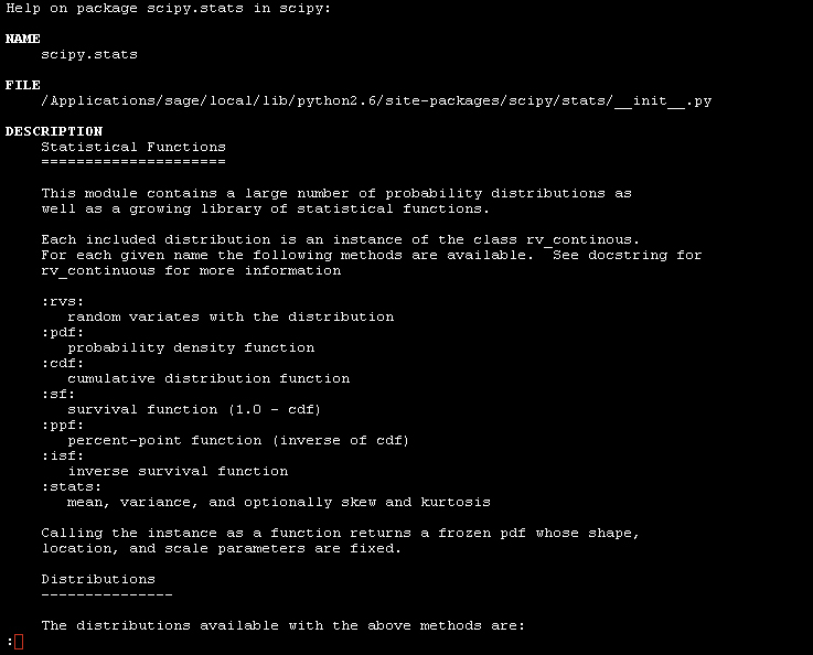
Note the colon (:) at the end of the screen—this is an old-school prompt. The system is in stand-by mode, expecting the user to issue a command (in the form of a single key). This also indicates that there are a few more pages of help following the given text. If we intend to read the rest of the help file, we may press Space bar to visit the next page. In this way we can visit the following manual pages on this topic. It is also possible to navigate the manual pages scrolling one line of text at a time, by using the up and down arrow keys. When we are ready to quit the help session, we simply press Q.

It is also possible to search the help contents for a given string. In that case, at the prompt, we press the (/) slash key. The prompt changes from a colon into a slash, and we proceed to input the keyword we would like to search for.

For example, is there a SciPy function that computes the Pearson kurtosis of a given dataset? At the slash prompt, we type in kurtosis and press enter. The help system takes us to the first occurrence of that string. To access successive occurrences of the string kurtosis, we press the N key (for next) until we find what we require. At that stage, we proceed to quit this help session (by pressing Q), and request more information on the function itself.

>>> help(scipy.stats.kurtosis)

The result is shown in the following screenshot:

At this point we would like to introduce you to another resource, which we will be using to generate graphs for the examples – the matplotlib libraries. It may be downloaded from its official web page, matplotlib.org, and installed following the usual Python motions. There is a good online documentation in the official web page, and we encourage the reader to dig deeper than the few commands that we will use in this book. For instance, the excellent monograph Matplotlib for Python Developers, Sandro Tosi, Packt Publishing, provides all we shall need and more. Other plotting libraries are available (commercial or otherwise), which aim to very different and specific applications. The degree of sophistication and ease of use of matplotlib makes it one of the best options for generation of graphics in scientific computing.

Once installed, it may be imported as usual, with import matplotlib. Among all its modules, we will focus on pyplot, which provides a comfortable interface with the plotting libraries. For example, if we desire to plot at this point a cycle of the sine function, we could execute the following code snippet:

import numpy
import matplotlib.pyplot
x=numpy.linspace(0,numpy.pi,32)
fig=matplotlib.pyplot.figure()
fig.plot(x, numpy.sin(x))
fig.savefig('sine.png')

We obtain the following plot:

Let us explain each command from the previous session. The first two commands are used to import numpy and matplotlib.pyplot as usual. We define an array x of 32 uniformly spaced floating point values from 0 to π, and define y to be the array containing the sine of the values from x. The command figure creates space in memory to store the subsequent plots, and puts in place an object of the form matplotlib.figure.Figure. The command plot(x, numpy.sin(x)) creates an object of the form matplotlib.lines.Line2D, containing data with the plot of x against numpy.sin(x), together with a set of axes attached to it, labeled according to the ranges of the variables. This object is stored in the previous Figure object. The last command in the session, savefig, saves the Figure object to whatever valid image format we desire (in this case, a Portable Network Graphics [PNG] image). If instead of saving to a file we desire to show on screen the result of the plot, we issue the fig.show() command. From now on, in any code that deals with matplotlib commands, we will leave the option of showing/saving open.

There are, of course, commands that control the style of axes, aspect ratio between axes, labeling, colors, the possibility of managing several figures at the same time (subplots), and many more options to display all sort of data. We will be discovering these as we progress with examples through the book.

In this chapter we have learned the benefits of using the combination of Python, NumPy, SciPy, and matplotlib as a programming environment for any scientific endeavor that requires mathematics; in particular, anything related to numerical computations. We have explored the environment, learned how to download and install the required libraries, used them for some quick computations, and figured out a few good ways to search for help.

In the next chapter we will guide you through basic object creation in SciPy, including the best methods to manipulate data, or obtain information from it.