Learning R for Geospatial Analysis

The R software can be downloaded from the R Project website at http://www.r-project.org/. The following screenshot shows the main page of this website:

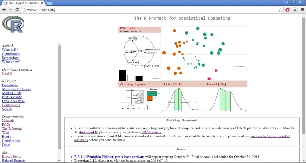
Perform the following steps to download R from the R Project website:

After downloading the file, follow the installation instructions. Note that if you are using a 64-bit version of Windows, you will be asked to select whether to install a 32-bit version, 64-bit version, or both. It is recommended that you use the 64-bit version in this case since it allows a single process to take advantage of more than 4 GB of RAM (this is helpful, for example, when loading a large raster file into memory).

Start R by navigating to Start | All Programs | R and choose the appropriate shortcut from there (such as R x64 3.1.0 when running the 3.1.0 64-bit version of R).

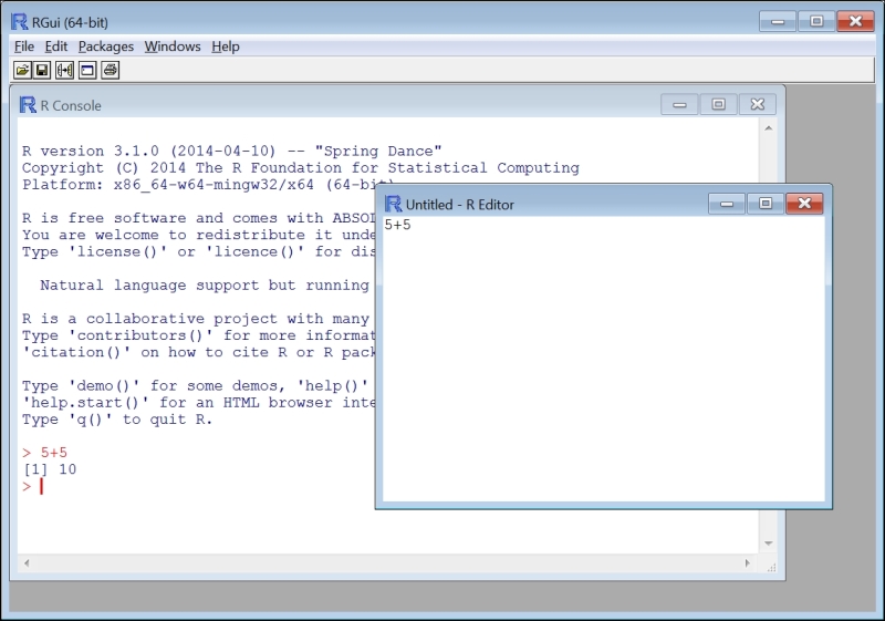
The main screen of the R Graphical User Interface (RGui) looks like the following screenshot:

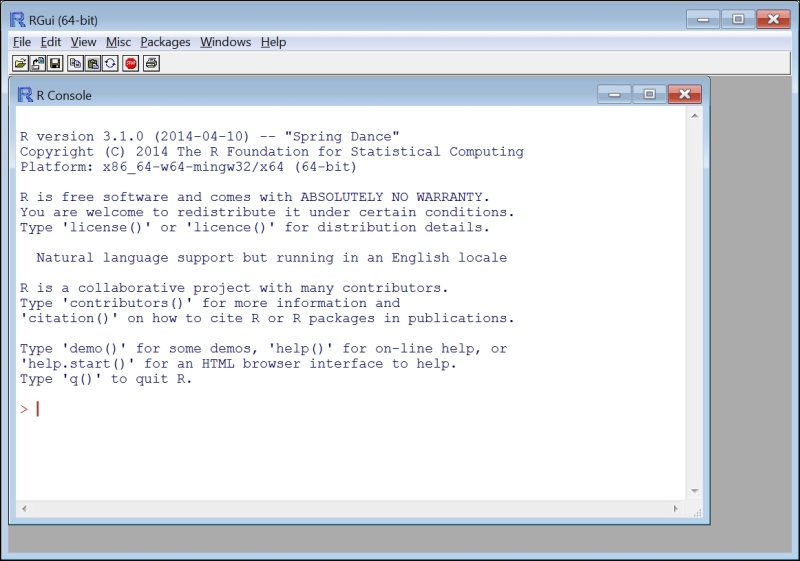
The window you see when starting the program, R Console, is the command line. The > symbol followed by a flashing cursor indicates that the system is waiting for instructions from the user. When the user types an expression into the command line and presses Enter, that expression is interpreted from the R language into the language that the computer processor understands, and the respective operation that expression entails is performed. As you may have noted, very few point-and-click menu options are found within the R environment as almost all operations are only accessible through code.

First, we will try simple calculations. For example, type the expression 5+5. The result 10 will appear on the next line followed by the > symbol, indicating that all instructions have been executed and the system is waiting for new ones:

> 5+5
[1] 10

What has just happened is that the expression 5+5 was interpreted and the respective instruction (add 5 and 5) was sent to the processor. The processor found the result (which is 10), which was then returned and printed in the command-line window. As we will see later, the result was saved neither in the RAM nor in the long-term computer memory, such as the hard disk. The meaning of the [1] part is that the result is a vector, with the first member being the number 10. Vectors will be covered in the next chapter.

Note that an R expression can be several lines long. For example, if we type 5* and press Enter, the symbol + appears on the next line, indicating that R is waiting for the remaining part of the expression (5 multiplied by ...):

> 5*
+ 2
[1] 10

If you change your mind and do not wish to complete the expression, you can press Esc to cancel the + mode and return to the command line. Pressing Esc can also be used to terminate the current process that is being executed. (We didn't get a chance to try that out yet since simple operations such as 5+5 are executed very quickly.)

Throughout this book, code sections display both the expressions that the user enters (following the > symbol) and the resulting output. Reading both the inputs and the outputs will make it easier to follow the code examples. If you wish to execute the code examples in R and to investigate what happens when modifying them (which is highly recommended), only the input expressions should be entered into the R interpreter (these are the expressions followed by the >, or + if the expression spans several lines, symbols). Therefore, copying and pasting the entire content of code sections directly from the book into the interpreter will result in errors, since R will try to execute the output lines. The input, in fact, will not be correctly interpreted either since input expressions include > and + symbols that are not part of the code. To make things easier, all code sections from this book are provided on the book's website as plain R code files.

Typing the expression 5+5 into the command line was easy enough. However, if we perform more complicated operations, we'll have to edit and save our code for later use. There are three main approaches to edit R code:

Using R's built-in editor is the simplest way to edit R code. In this case, you don't need to use any software other than R. To open the code editor, simply navigate to File | New script from R's menu. A blank text window will open. You can type code in this window and execute it by clicking on Ctrl + R, either after selecting the code section that you want to execute (the selected section will be sent to the interpreter) or by placing the cursor on the line that you want to execute (that line will be sent to the interpreter).

The following screenshot shows the way RGui appears with both a command-line window and a code editor window:

You can save the R code that you have written to a file at any time (File | Save as...) in order to be able to work on it another day. An R code file is a plain text file, usually with the suffix .R. To open an existing R code file, simply select it after navigating to the File | Open script... menu.

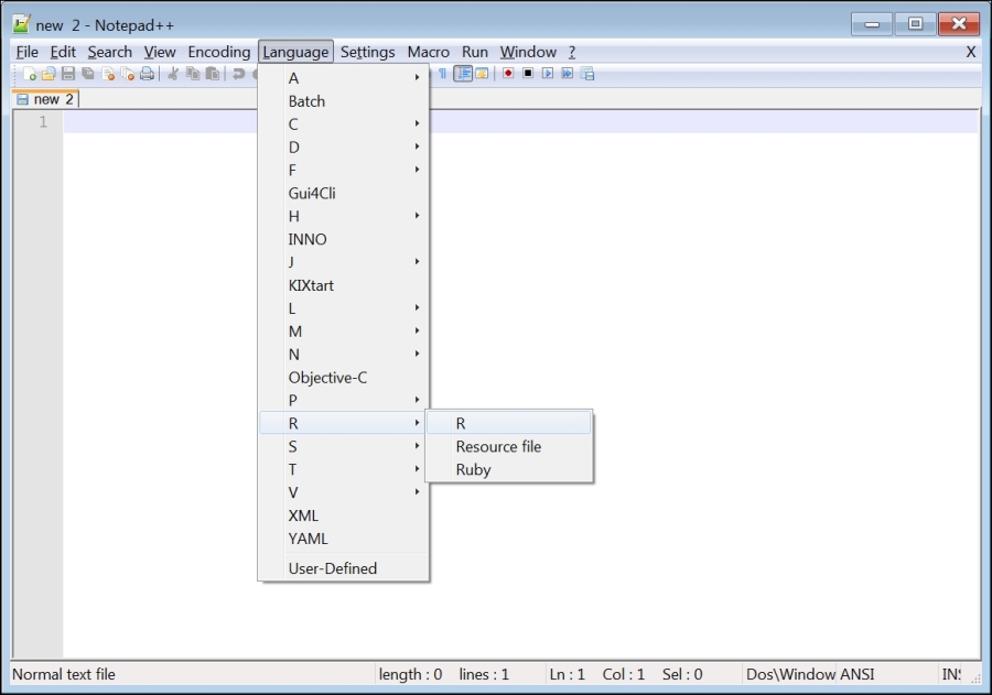
It is sometimes easier to use other text editors since they provide more options than R's basic text editor. For example, one can edit R code in the all-purpose Notepad++ text editor, which is available for free at http://notepad-plus-plus.org/. Notepad++ can be customized to edit code written in different programming languages (including R). By selecting the appropriate language, the specific function names and operators of that language will be highlighted in different colors for easier interpretation by the user.

The following screenshot shows Notepad++ with the menus used to select the R programming language:

A code section can be transferred to the R interpreter simply by copying it from the text editor and then pasting into the R command line. To automatically pass code into the R interpreter (such as by clicking Ctrl + R), it might be necessary to install an add-on component such as the NppToR software for Notepad++ (which is freely available at http://sourceforge.net/projects/npptor/), or use a text editor such as Tinn-R (which is freely available at http://sourceforge.net/projects/tinn-r/) that has this capability built in.

The most sophisticated way of editing R code is to use an IDE, where an advanced text editor and the R interpreter portions are combined within a single window (much like in RGui itself), in addition to many other advanced functions that may be of help in programming and are not found in RGui. These can include automatic code completion, listings of libraries and functions, automatic syntax highlighting (to read code and output more easily), debugging tools, and much more.

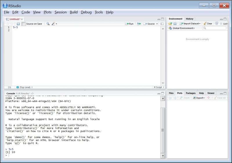
RStudio is an IDE designed specifically for R, and it is the recommended way of editing R code. You will quickly discover that even without using any of the advanced options, code editing in RStudio is more convenient than the previously mentioned alternatives. RStudio can be freely downloaded from www.rstudio.com.

When you open RStudio, you will see the R command-line window and several additional utility panes that can display the code editor, help files, graphic output, and so on, during the course of working in R. To open a new R code file, navigate to File | New File | R Script. A code editing window, such as the one shown in the following screenshot, will appear:

In RStudio, code can be sent from the editor window into the command-line window in the same way as in RGui, that is, by pressing Ctrl + R either on a code section or on a single line of code. You can quickly switch to the code editor or to the command-line pane by clicking on it with the mouse or by pressing Ctrl + 1 or Ctrl + 2, respectively. You can also have several R code files open in different tabs within the code editor pane.

More details can be found on the RStudio website (www.rstudio.com) or in other resources such as Mark P.J. van der Loo and Edwin de Jonge's book Learning RStudio for R Statistical Computing, Packt Publishing (2012).

The standard arithmetic operators in R are as follows:

The following examples demonstrate the usage of these operators:

> 5+3
[1] 8
> 4-5
[1] -1
> 1*10
[1] 10
> 1/10
[1] 0.1
> 2^3
[1] 8

Parentheses can be used to construct more elaborate expressions, as follows:

> 2*(3+1)
[1] 8
> 5^(1+1)
[1] 25

It is better to use parentheses even when it is not required to make the code clearer.

Another very useful symbol is #. All code to the right of this symbol is not interpreted. Let's take a look at the following example:

> 1*2 # *3
[1] 2

The # symbol is helpful for adding comments within the code to explain what each code segment does, for other people (or oneself, at a later time of reference) to understand it:

> 5+5 # Adding 5 and 5
[1] 10

Note that R ignores spaces between the components of an expression:

> 1+  1
[1] 2

Conditions are expressions that have a yes/no answer (the statement can be either true or false). When interpreting a conditional expression, R returns a logical value, either TRUE for a true expression or FALSE for a false expression. A third option, NA, which stands for Not Available, is used when there is not enough information to determine whether the expression is true or false (NA values will be discussed in the next chapter).

The logical operators in R are summarized as follows:

For example, we can use condition operators to compare between two numbers as follows:

> 1<2
[1] TRUE
> 1>2
[1] FALSE
> 2>2
[1] FALSE
> 2>=2
[1] TRUE
> 2!=2
[1] FALSE

The and (&) and or (|) operators can be used to construct more complex expressions as follows:

> (1<10) & (10<100)
[1] TRUE
> (1<10) & (10>100)
[1] FALSE
> (1<10) | (10<100)
[1] TRUE
> (1<10) | (10>100)
[1] TRUE

As you can see in the preceding examples, when the expressions at both the sides of the & operator are true, TRUE is returned; otherwise, FALSE is returned (refer to the first two expressions). When at least one of the expressions at either side of the | operator is true, TRUE is returned; otherwise, FALSE is returned (refer to the last two expressions).

Two other useful conditional operators (== and !=) are used for testing equality and inequality, respectively. These operators are opposites from one another since a pair of objects can be either equal or non-equal to each other.

> 1 == 1
[1] TRUE
> 1 == 2
[1] FALSE
> 1 != 1
[1] FALSE
> 1 != 2
[1] TRUE

As you can see in the preceding examples, when using the == operator, TRUE is returned if the compared objects are equal; otherwise FALSE is returned (refer to expressions 1 and 2). With != it is the other way around (refer to expressions 3 and 4).

The last operator that we are going to cover is the not operator (!). This operator reverses the resulting logical value, from TRUE to FALSE or from FALSE to TRUE. This is used in cases when it is more convenient to ask whether a condition is not satisfied. Let's take a look at the following example:

> 1 == 1
[1] TRUE
> !(1 == 1)
[1] FALSE
> (1 == 1) & (2 == 2)
[1] TRUE
> (1 == 1) & !(2 == 2)
[1] FALSE

In mathematics, a function is a relation between a set of inputs and a set of outputs with the property that each input is related to exactly one output. For example, the function y=2*x relates every input x with the output y, which is equal to x multiplied by 2. The function concept in R (and in programming in general) is very similar:

The most common (and the most useful) expressions in R are function calls. In fact, we have been using function calls all along, since the arithmetic operators are functions as well, which becomes apparent when using a different notation:

> 3*3
[1] 9
> "*"(3,3)
[1] 9

A function is essentially a predefined set of instructions. There are plenty of built-in functions in R (functions that are automatically loaded into memory when starting R). Later, you will also learn how to use functions that are not automatically loaded, and how to define your own functions.

As you might have guessed from the previous example, a function call is composed of the function name, followed by the function's arguments within parentheses and separated by commas. For example, the function sqrt returns the square root of its argument:

> sqrt(16)
[1] 4

> Sqrt(16)
Error: could not find function "Sqrt"

Error messages are printed when for some reason it is impossible to execute the expression that we have sent to the interpreter. For example, this can happen when one of the objects we refer to does not exist (refer to the preceding information box). Another example is trying to pass an inappropriate argument to a function. In R, character values are delimited by quotes. Trying to call a mathematical function on a character understandably produces an error:

> "oranges" + "apples"
Error in "oranges" + "apples" : non-numeric argument to binary op$

Warning messages are returned when an expression can be interpreted but the system suspects that the respective employed method is inappropriate. For example, the square root of a negative number does not yield a number within the real number system. A Not a Number (NaN) value is returned in such a case, along with a warning:

> sqrt(-2)
[1] NaN
Warning message:
In sqrt(-2) : NaNs produced

R has a set of predefined symbols to represent special constant values, most of which we already mentioned:

A help page on every function in R can be reached by using the ? operator (or the help function). For example, the following expression opens the help page for the sqrt function:

> ?sqrt

The same result is achieved by typing help(sqrt).

The structure of all help files on functions is similar, usually including a short description of what the function does, the list of its arguments, usage details, a description of the returned object, references, and examples. The help pages can seem intimidating at first, but with time they become clearer and more helpful for reminding oneself of the functions' usage details.

Another important source of information on R is the Internet. Entering a question or a task that we would like to perform (such as Googling r read raster file) into a web search engine usually yields a surprising amount of information from forums, blogs, and articles. Using these resources is inevitable when investigating new ways to utilize R.

R is an object-oriented language; accordingly, everything in R is an object. Objects belong to classes, with each class characterized by certain properties. The class to which an object belongs to determines the object's properties and the actions we can do with that object. To use an analogy, a gray Mitsubishi Super-Lancer model 1996 object belongs to the class car. It has specific attributes (such as color, model, and manufacturer) for each of the data fields a car object has. It satisfies all criteria that the car class entails; thus, the actions that are applicable to cars (such as igniting the engine and accelerating or using the breaks) are also meaningful with that particular object. In much the same way, a multi-band raster object in R will obligatorily have certain properties (such as the number of rows and columns, and resolution) and applicable actions (such as creating a subset of only the first band or calculating an overlay based on all bands).

All objects that are stored in memory can be accessed using their names, which begin with a character (without quotes; some functions, such as all arithmetic and logical operators can be called using their respective symbol within quotes, such as in "*" as we saw earlier). For example, sqrt is the name of the square root function object; the class to which this object belongs is function. When starting R, a predefined set of objects is loaded into memory, for example, the sqrt function and logical constant values TRUE and FALSE. Another example of a preloaded object is the number :

> pi
[1] 3.141593

The class function returns the class name of the object that it receives as an argument:

> class(TRUE)
[1] "logical"
> class(1)
[1] "numeric"
> class(pi)
[1] "numeric"
> class("a")
[1] "character"
> class(sqrt)
[1] "function"

From the point of view of a typical R user, all objects we handle in R can be divided into two groups: data structures (which hold data) and functions (which are used to perform operations on the data).

The basic components of all data structures are constant values, usually numeric, character, or logical (the last code section shows examples of all three). The simplest data structure in R is a vector, which is covered in Chapter 2, Working with Vectors and Time Series. Later, we'll see how more complex data structures are essentially collections of the simpler data structures. For example, a raster object in R may include two numeric vectors (holding the raster values and its dimensions) and a character vector (holding the Coordinate Reference System (CRS) information). The object-oriented nature of the language makes things easier both for the people who define the data structure classes (since they can build upon predefined simpler classes, rather than starting from the beginning) and for the users (since they can utilize their previous knowledge of the simpler data structure components to quickly understand more complex ones).

Objects of the second type—functions—are typically used to perform operations on data structures. A function may have its influence limited to the R environment, or it may invoke side effects affecting the environment outside of R. All functions we have used until now affect only the R environment; a function to save a raster file, for example, has an external effect—it influences the data content of the hard drive.

Finally, let's take a look at a complete code section that performs a simple spatial analysis operation:

> library(raster)
> r = raster("C:\\Data\\rainfall.tif")
> r[120, 120] = 1000
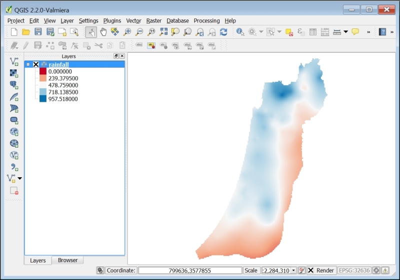
> writeRaster(r, "C:\\Data\\rainfall2.tif")

The task that this code performs is to read a raster file, rainfall.tif, from the disk (look at the following screenshot to see its visualization in QGIS), change one of its values (the one at row 120 line 120, into 1000) and write the resulting raster to a different file.

Do not worry if you do not understand all the lines of code given in the beginning of this section. They will become clear by the time you finish reading Chapter 4, Working with Rasters. Briefly, the first line of code tells R to load the set of functions that are used to work with rasters (called the raster package), such as the raster and writeRaster functions that we use here to read and write raster files. In the second line, we read the requested file and load it into memory. In the third line of code, we assign the value 1000 to the specified pixel of that raster. The fourth line of code writes the new (modified) raster to the disk.

The task indeed sounds simple, but when we use desktop GIS software, it may not be easy to perform through the menus and dialog box system (where direct access to raster values may be unavailable). For example, we may have to create a new point feature over the pixel that we want to change (120,120) in raster A, convert it to a raster B (with the value of 1 at the (120,120) pixel and 0 in all other pixels), and then use an overlay tool to say that we want the pixel in raster A that overlays the value of 1 in raster B to have the value of 1000, while all other pixels retain their original values. Finally, we might need to use an additional toolbox to export the new raster. However, what if we need to perform this operation on several files or repeatedly on a given file as new information comes in?

Generally speaking, when we use programming rather than menu-based interfaces, the steps we have to take may seem less intuitive (writing code rather than scrolling, clicking with the mouse, and filling out dialog boxes). However, we have much more power with giving the computer specific instructions. The beauty of using programming for data analysis, and using R for geospatial analysis in particular, is not only that we gain greater efficiency through automation, but also that we get closer to the data and discover a wide range of new possibilities to analyze it, some of which may not even come to mind when we use a predefined set of tools or menus.