Download code from GitHub
In this chapter, we present recipes covering the following topics:
- Installation issues:
- How to install Julia in different environments
- How to compile your own Julia binaries
- How to use Julia in the cloud in Amazon Web Services (AWS) using Cloud9
- Basic usage of Julia:
- The various ways you can the start-up of Julia
- How to set up Julia to work with multiple cores
- How to perform the standard steps comprising a daily workflow using the Julia command line (the Julia language shell also referred to as the Julia REPL)
- How to display computational results in Julia
- How to manage packages
- More advanced configurations of Julia usage:
- How to launch Julia in Jupyter Notebook
- How to use Julia with JupyterLab
- How to connect to Jupyter Notebook in Terminal-only cloud environments
A key condition for successfully working with any programming language is the careful configuration of the development environment. Julia, being an open source language, offers integration with several popular tools. This means that developers have a number of alternatives at hand when setting up the complete Julia toolbox.
The first decision to be made is the choice of Julia distribution. Available options include binary and source code forms. For non-typical hardware configurations, or when one wishes to use all the latest compiler features, Julia source code can be downloaded. Another decision concerns which compiler to use in order to build Julia (GCC or Intel) and whether to link Julia against Intel's mathematical libraries.
The second decision lies in the choice of IDE. Julia can be integrated with various editors, with Atom plus the Juno plugin being the most popular choice. Yet another option is to use a browser-based Julia IDE—Jupyter Notebook, JupyterLab, or Cloud9.
In this chapter, we discuss all the preceding options and show how to set up the complete Julia programmer's environment, along with the most important technical tips and recommendations.
The goal of this recipe is to present how to install and configure the Julia environment with the development toolbox. We show basic installation instructions for Linux and Windows.
In this recipe, we present how to install and configure Julia on Windows and Linux.
All Linux examples in this book have been tested on Linux Ubuntu 18.04.1 LTS and Windows 10. All Linux Ubuntu commands have been run as the user ubuntu. Please note that users of other Linux distributions will need to update their scripts (for example, Linux distributions from the Red Hat family use yum instead of apt).
For Windows examples in this book, we use Windows 10 Professional.
Note
In the GitHub repository for this recipe you will find the commands.txt file that contains the presented sequence of shell commands.
For most users, the recommended way to start with Julia is to use a binary version.
In this section, we present the following options:
- Installing Julia on Linux Ubuntu
- Installing Julia on Windows
Installing the binary release is the easiest way to proceed with Julia on Linux. Here, we show how to install Julia on Ubuntu, although the steps will be very similar for other Linux distributions.
Before the installation and use of Julia, we recommend installing a standard set of build tools for the Linux platform. Although this is not required for running Julia itself, several Julia package installers assume that the standard build tools set is present on the operating system. Hence, run the following commands in bash:
$ sudo apt update
$ sudo apt -y install build-essential
In order to install Julia, simply download the binary archive from julialang.org, uncompress it, and finally create a symbolic link named Julia. These steps are shown in the following three bash commands (we assume that these commands are run in the /home/ubuntu folder):
$ wget https://julialang-s3.julialang.org/bin/linux/x64/1.0/julia-1.0.1-linux-x86_64.tar.gz
$ tar xvfz julia-1.0.1-linux-x86_64.tar.gz
$ sudo ln -s /home/ubuntu/julia-1.0.1/bin/julia /usr/local/bin/julia
Please note that the last command creates a symbolic link to the Julia binaries. After this installation, it is sufficient to run the julia command in the OS shell to start working with Julia.
Please note that on the Julia web page (https://julialang.org/downloads/), a newer version of the installer could be available. You can update the preceding script accordingly by simply updating the filename. Additionally, nightly build Julia versions are available on the preceding website. These versions are only recommended for testing new language features.
The most convenient way to install Julia on Windows is by using the binary version installer available from the JuliaLang website.
The following steps are required to install Julia on a Windows system:
- Download the
Windows Self-Extracting Archive (.exe)fromhttps://julialang.org/downloads/. It is recommended to select the64-bitversion. - Run the downloaded
*.exefile to unpack Julia. We recommend extracting Julia into a directory path that does not contain any spaces, for example,C:\Julia-1.0.1. - After a successful installation, a Julia shortcut will be added to your start menu—at this point, you can select the shortcut to see whether Julia loads correctly.
- Add
julia.exeto your system path, as follows:- Open Windows Explorer, right-click on the
This PCcomputer icon, and selectProperties. - Click
Advanced system settingsand go toEnvironmentVariables.... - Select the
Pathvariable and clickEdit.... - To the variable value,add
C:\Julia-1.0.1\bin(in this instruction, we assume that Julia has been installed toC:\Julia-1.0.1). Please note that, depending on your Windows version, there is either onePathvalue per line or a semicolon;is used to separate values in thePathlist. - Click
OKto confirm. Now, Julia can be run anywhere from the console.
- Open Windows Explorer, right-click on the
When adding julia.exe to your system path, please note that there are two variable groups on this screen, User variablesandSystem variables. We recommend using User variables. Please note that adding julia.exe to the system Path makes it possible for other tools, such as Juno, toautomatically locate Julia (Juno also allows for manual Julia path configuration—this can be found in the option marked Packages | Julia client | Settings).
Note
For the most convenient workflow, we recommend installing the ConEmu terminal emulator for Windows users. The steps to install ConEmu on your Windows system are as follows:
- Go to theConEmu website (http://conemu.github.io/)and click the
Downloadlink. SelectDownload ConEmu Stable Installer. - Once you download the
*.exefile, run it to install ConEmu. Select the 64-bit version in the installer; other settings can keep their default values. - Once ConEmu is installed, a new link in the start menu and on the desktop will be created.
- During the first application run, ConEmu asks about color settings—just stay with the defaults. Run ConEmu, type
julia, and press Enter, and you should see a Julia prompt.
Those users who want to try Julia without the installation process should try JuliaBox.
JuliaBox is a ready-made pre-installed Julia environment accessible from the web browser. It is available at https://juliabox.com/. You can use this version to play with a preconfigured and installed version of the Julia environment. Julia is available in a web browser via the Jupyter Notebook environment. The website is free to use, though it does require registration. JuliaBox comes with a set of pre-configured popular Julia libraries and is therefore ready for immediate use. This is an ideal solution for people wanting to try out the language or for using Julia inside a classroom.
Excellent documentation on how to install Julia on various systems can be found on the JuliaLang website: https://julialang.org/downloads/platform.html.
Integrated Desktop Environments (IDEs) are integrated tools that provide a complete environment for software development and testing. IDEs provide visual support for the development process, including syntax highlighting, interactive code editing, and visual debugging.
Before installing an IDE, you should have Julia installed (either from binaries or source), following the instructions given in previous recipes.
The three most popular Julia IDEs are Juno, Microsoft Visual Studio Code, and Sublime Text. In subsequent sections, we discuss the installation process for each particular IDE.
Juno is the recommended IDE for Julia development.The Juno IDE is available athttp://junolab.org/. However, Juno runs as a plugin to Atom (https://atom.io/). Hence, in order to install Juno, you need to take the following steps:
- Make sure that you have installed Julia and added it to the command path (following the instructions given in previous sections).
- Download and install Atom, available athttps://atom.io/.
- Once the installation is complete, Atom will start automatically.
- PressCtrl + , (Ctrl key + comma key) to open the Atom settings screen.
- Select the
Installtab. - In the
Search packagesfield, typeuber-junoand pressEnter. - You will see the
uber-junopackage developed by JunoLab—clickInstallto install the package. - In order to test your installation, click the
Show consoletab on the left.
Please note that when being run for the first time from Atom, Julia takes longer to start. This happens because Juno is installed along with several other packages that are being compiled before their first use.
Note that at the time of publishing this book the Microsoft Visual Studio Code does not yet support Julia 1.0. However, since we believe that this support will be available very soon, we provide the instructions below.
The Microsoft Visual Studio Code editor can be obtained fromhttps://code.visualstudio.com/.Simply download the installer executable and install using the default settings. After launching Visual Studio Code, perform the following steps:
Click
Extensionstab (or press Ctrl + Shift + X).In the search box, type
julia. You will seeJulia Language Supporton the list. Click the greenInstallbutton to start the installation.Click
File|New Fileto create a new, empty file.Click
File|Save As...to save the newly created file. In theSave As...typeJulia(please note that the file type list might not be sorted alphabetically and Julia type might be at the bottom of the list).Open the Terminal tab and issue the
juliacommand.
After following these steps, you will have a Julia file open in the editor and an active Julia Terminal. PressingCtrl + Enter will now send the currently highlighted code line to the Terminal to execute it.
Another option for the IDE is utilizing the functionality of Sublime Text:
- Next, the simplest thing to add is a custom build system for Julia (
Tools|Build System|New Build System):
{
    "cmd": ["ConEmu64", "/cmd", "julia -i", "$file"],
    "selector": "source.julia"
}- Now, you can execute an opened Julia script by pressingCtrl + B in the console in interactive mode (
-iswitch).
The preceding example assumes thatConEmu64andjuliaare defined in the search path.
The only inconvenience of this method is that if there is an error in the Julia script, the console will be immediately terminated (a cleaner way to test your scripts is to keep your Terminal with Julia open) and use theinclude command, as explained in the recipe Useful options for interaction with Julia in this chapter.
For integration with other editors and IDEs, take a look at the https://github.com/JuliaEditorSupport project.
On some computational environments, no desktop is available and so users may want to use Julia in a text-only mode.
Before installing Julia support for text editors, you should have Julia preinstalled (either from binaries or source), in accordance with the instructions given in previous recipes.
The three most popular text editors used by Julia developers include Nano, Vim, and Emacs. Here, we provide some hints on how to configure Julia with these popular text-mode editors. All the following examples have been tested with Ubuntu 18.0.4.1 LTS.
Nano is a popular Linux text editor for beginners. By default, nano does not provide syntax highlighting for Julia. However, this can easily be remedied by adding appropriate lines to the .nanorc configuration file, which should be located in the user's home directory. The following commands will update the .nanorc file with the appropriate syntax coloring for Julia. Firstly, download syntax highlighting for Julia (https://stackoverflow.com/questions/35188420/syntax-highlighting-support-for-julia-in-nano):
$ wget -P ~/ https://raw.githubusercontent.com/Naereen/nanorc/master/julia.nanorcSecondly, add highlighting to the nano configuration file, using the bash command, as follows:
$ echo include \"~/julia.nanorc\" >> ~/.nanorcIn order to configure Julia for Vim, you need to use the files available at the git://github.com/JuliaEditorSupport/julia-vim.git project. All you need to do for this is to copy them to the Vim configuration folder. On a Linux platform, this can be achieved by running the following commands:
git clone git://github.com/JuliaEditorSupport/julia-vim.git
mkdir -p ~/.vim
cp -R julia-vim/* ~/.vim
Once julia-vim is installed, one interesting feature is the support for LaTeX-style special characters. Try running vim file.jl and type \alpha, then press the Tab key. You will observe the text changing to the corresponding α character.
Further information and other useful options can be found on the julia-vim project website at git://github.com/JuliaEditorSupport/julia-vim.git.
Since Emacs is not present by default in Ubuntu, the following instruction assumes that it has been installed by the sudo apt install emacs25 command. In order to configure Emacs support for Julia, you need to activate the julia-mode mode. This can be achieved with the following bash commands:
wget -P ~/julia-emacs/ https://raw.githubusercontent.com/JuliaEditorSupport/julia-emacs/master/julia-mode.el
echo "(add-to-list'load-path \"~/julia-emacs\")" >> ~/.emacs
echo "(require'julia-mode)" >> ~/.emacs
For integration with other editors and IDEs, take a look at the Julia Editor Support project, which is available at https://github.com/JuliaEditorSupport.
Building Julia allows you to test the latest developments and includes bug fixes. Moreover, when Julia is compiled, it is optimized for the hardware that the compilation is performed on. Consequently, building Julia from source code is the recommended option for those production environments where performance is strongly affected by platform-specific features. These instructions will also be valuable for those Julia users who would like to check out and experiment with the latest source versions from the Julia Git repository.
In the following examples, we show how to install and build a stable version of Julia 1.0.1.
All the following examples have been tested on Ubuntu 18.04.1 LTS.
Here is a list of steps to be followed:
- Open the console and install all the prerequisites. Please refer to the following script (run each shell command shown as follows):
$ sudo apt update
$ sudo apt install --yes build-essential python-minimal gfortran m4 cmake pkg-config libssl-dev
- Download the source code (run each shell command shown as follows; we assume that the commands are run in your
homefolder):
$ git clone git://github.com/JuliaLang/julia.git
$ cd julia
$ git checkout v1.0.1
In this section, we describe how to build Julia in three particular variations:
The libraries from Intel (MKL and LIBM) provide an implementation for a number of mathematical operations optimized for Intel's processor architecture. In particular, the Intel MKL library contains optimized routines for BLAS, LAPACK, ScaLAPACK, sparse solvers, fast Fourier transforms, and vector math (for more details see https://software.intel.com/en-us/mkl). On the other hand, the Intel LIBM library provides highly optimized scalar math functions that serve as direct replacements for the standard C calls—this includes optimized versions of standard math library functions, such as exp, log, sin, and cos). More information on Intel LIBM can be found at https://software.intel.com/en-us/articles/implement-the-libm-math-library.
Before running each of the recipes, please make sure that you are inside the folder where you ran the checkout command for Julia (see the Getting ready section).
Once you have followed the steps in the Getting ready section and Julia has been checked out from the Git repository, perform the following steps:
$ make-j$((`nproc`-1))1>build_log.txt 2>build_error.txtThe build logs will be available in the build_log.txt and build_error.txt files.
- Once the Julia environment has been built, you can run the
./juliacommand and useversioninfo()to check your installation:
julia> versioninfo()
Julia Version 1.0.1
Commit 0d713926f8* (2018-09-29 19:05 UTC)
Platform Info:
  OS: Linux (x86_64-linux-gnu)
  CPU: Intel(R) Xeon(R) Platinum 8124M CPU @ 3.00GHz
  WORD_SIZE: 64
  LIBM: libopenlibm
  LLVM: libLLVM-6.0.0 (ORCJIT, skylake)
Once you have followed the steps in the Getting ready section and Julia has been checked out from the Git repository, perform the following the steps:
- The MKL library is freely available from Intel. In order to get access to Intel MKL, you need to submit a form on Intel's website at https://software.intel.com/en-us/mkl.
- Once the form has been completed, you receive an MKL download link (please note that the actual filenames may be different in the library version you obtain).
- Execute the following commands to install MKL:
$ cd ~
# Get link from MKL website
$ wget http://registrationcenter-download.intel.com/[go to Intel MKL web site to get link]/l_mkl_2019.0.117.tgz
$ tar zxvf l_mkl_2019.0.117.tgz
$ cdl_mkl_2019.0.117
$ sudobash install.sh
- Once the Intel MKL library is installed, you can build Julia (run each shell command as shown):
cd ~/julia echo"USEICC = 0" >> Make.user echo"USEIFC = 0" >> Make.user echo"USE_INTEL_MKL = 1" >> Make.user echo"USE_INTEL_LIBM = 0" >> Make.user source /opt/intel/bin/compilervars.sh intel64 make-j$((`nproc`-1))1>build_log.txt 2>build_error.txt
The build logs will be available in the build_log.txt and build_error.txt files.
- Once Julia is successfully built, run the
./juliacommand to start it. - Use
versioninfo()to check the status of Julia. Information about the MKL status is available from theENV["MKL_INTERFACE_LAYER"]system variable. Take a look at a sample screen, as follows:
julia> versioninfo()
Julia Version 1.0.1
Commit 0d713926f8* (2018-09-29 19:05 UTC)
Platform Info:
  OS: Linux (x86_64-linux-gnu)
  CPU: Intel(R) Xeon(R) Platinum 8124M CPU @ 3.00GHz
  WORD_SIZE: 64
  LIBM: libopenlibm
  LLVM: libLLVM-6.0.0 (ORCJIT, skylake)

julia> ENV["MKL_INTERFACE_LAYER"]
"ILP64"
Note
Please note that if you build Julia with MKL, whenever you start a new Linux session you need to tell Julia where the Intel compilers are so that it can properly find and use the MKL libraries. This is done by executing the following bash command:
$source /opt/intel/bin/compilervars.sh intel64 The preceding command needs to be executed each time prior to launching the julia process in a new environment.
Once you have followed the steps in the Getting ready section and Julia has been checked out from the Git repository, perform the following steps:
- Acquire an Intel Parallel Studio XE (https://software.intel.com/en-us/c-compilers/ipsxe) license, which entitles you to use theIntel C++ compilers (https://software.intel.com/en-us/c-compilers) along with the Intel Math Library(Intel LIBM, available at https://software.intel.com/en-us/node/522653).
- Once you acquire the license, together with a download link from Intel, download and install the software by running the shell commands given as follows (please note that the actual filenames may be different in the library version you obtain):
$ cd ~
# Get the link from Intel C++ compilers website
$ wget http://[go to Intel to get link]/parallel_studio_xe_2018_update3_professional_edition.tgz
$ tar zxvf parallel_studio_xe_2018_update3_professional_edition.tgz
$ cd parallel_studio_xe_2018_update3_professional_edition
$ sudobash install.sh
- Select the MKL among the installation options in Intel Parallel Studio XE.
- Build Julia (run each shell command as shown):
cd ~/julia echo"USEICC = 0" >> Make.user echo"USEIFC = 0" >> Make.user echo"USE_INTEL_MKL = 1" >> Make.user echo"USE_INTEL_LIBM = 1" >> Make.user source /opt/intel/bin/compilervars.sh intel64 make-j$((`nproc`-1))1>build_log.txt 2>build_error.txt
The build logs will be available in thebuild_log.txt and build_error.txt files.
- Once Julia has been compiled, you can start it with the
./juliacommand and use theversioninfo()command—theLIBMparameter should point tolibimf.
Note
Please note that if you build Julia with MKL/LIBM, when you start a new Linux session, you need to tell Julia where Intel compilers are so it can properly find and use MKL/LIBM libraries:$source /opt/intel/bin/compilervars.sh intel64
The preceding command needs to be executed each time before launching the julia process in a new environment (hence, one might want to add that command to the ~/.profile start-up file).
For the highest performance, it is recommended to compile Julia with the Linux Intel MKL (Intel MKL is available at https://software.intel.com/en-us/mkl) drivers, which are available for free from Intel. The numerical performance can also be enhanced by using the Intel Math Library (Intel LIBM is available at https://software.intel.com/en-us/node/522653). However, LIBM can only be obtained with the Intel C++ compilers (see https://software.intel.com/en-us/c-compilers), which are free for academic and open source use but paid otherwise. Therefore, some users might be interested in building Julia with MKL, but without LIBM.
Please note that in all the scenarios outlined, we use GNU compilers rather than Intel compilers—even when using Intel's MKL and LIBM libraries. If you want to use Intel's compilers, you need to set the appropriate options in the Make.user file (that is, change USEICC = 0 and USEIFC = 0 to USEICC = 1 and USEIFC = 1). However, Intel compilers are currently not supported by Julia compiler scripts (see https://github.com/JuliaLang/julia/issues/23407).
Once Julia is installed on your system, it can be run by giving the full path to the Julia executable (for example,~/julia/julia). This is not always convenient—many users simply want to typejuliato get Julia running:
$ sudoln-s /home/ubuntu/julia/usr/bin/julia /usr/local/bin/juliaThe preceding path assumes that you installed Julia as theubuntuuser in your home folder. If you have installed Julia to a different location, please update the path accordingly.
If you want to build Julia in a supercomputing environment (for example, Cray), please follow the online tutorial written by one of the authors of this book, available at https://github.com/pszufe/Building_Julia_On_Cray_and_Clusters.
Cloud9 is an integrated programming environment that can be run inside a web browser. We will demonstrate how to configure this environment for programming with Julia. The web page of Cloud9 can be reached at https://aws.amazon.com/cloud9/.
In order to use Cloud9, you must have an active Amazon Web Services (AWS) account and log in to the AWS management console.
Cloud9 can create a new EC2 instance running Amazon Linux or can connect to any existing Linux server that allows SSH connections and has Node.js installed.In order to start working with Julia on Cloud9, complete the following steps:
- Prepare a Linux machine with Julia installed (you can follow the instructions in the previous sections).
- Install Node.js. In Ubuntu 18.04.1 LTS, for example, the only step needed is to run
sudo apt install nodejs. - Make sure that your server is accepting external SSH connections. For an AWS EC2 instance, you need to configure the instance security group to accept SSH connections from
0.0.0.0/0—in order to do this, click on the EC2 instance in the AWS console, selectSecurity Groups|Inbound|Edit,and add a new rule that accepts all traffic.
Once you have prepared a server with Julia and Node.js, you can take the following steps to use Cloud9:
- In the AWS console, go to the Cloud9 service and create a new environment.
- Select the
Connect and run in remote server (SSH)option. - For the username, type
ubuntuif you use Ubuntu Linux, orec2-userif you are running Amazon Linux, CentOS, or Red Hat (please note that this recipe has been tested with Ubuntu). - Provide the hostname (public DNS) of your EC2 instance.
- Configure SSH authorization.
- In the
Environment settingsscreen, selectCopy key to clipboardto copy the key. - Open an SSH connection to your remote server in a Terminal window.
- Execute the
nano ~/.ssh/authorized_keyscommand to edit the file. - Create an empty line and paste the public key content that you have just copied.
- PressCtrl + Xand confirm the changes withYto exit.
- Now, you are ready to click the
Next stepbutton in the Cloud9 console. Cloud9 will connect to your server and automatically install all the required software. After a few minutes, you will see your Cloud9 IDE. By default, Cloud9 does not support running programs in Julia. - Go to the
Runmenu and selectRun with|New runner. Type the following contents:
 {
"cmd" : ["julia", "$file", "$args"],
"info" : "Started $project_path$file_name",
"selector" : "source.jl"
}- Save the file as
JuliaRunner.run. - Now, pressing the
Runbutton will run your Julia*.jlfile.
The Cloud9 environment runs in your web browser. The browser opens a REST connection back to Cloud9's server, which in turn opens an SSH connection to your Linux instance (see the following diagram). This functionality will, in fact, run with any Linux server that accepts incoming connections from Cloud9 (more details on configuring other Linux servers with Cloud9 can be found at https://docs.aws.amazon.com/cloud9/latest/user-guide/ssh-settings.html):

Please note that this means that the EC2 instance supporting Cloud9 should allow incoming connections from the AWS Cloud9 infrastructure. In production environments, we recommend limiting traffic to the EC2 instance (viaSecurityGroup) to the IP ranges defined for Cloud9. Detailed instructions can be found in Cloud9's documentation: https://docs.aws.amazon.com/cloud9/latest/user-guide/ip-ranges.html.
The Cloud9 environment is being continuously updated by AWS; new features are being added frequently. For the latest documentation, we recommend looking at AWS Cloud9's user guide, available athttps://docs.aws.amazon.com/cloud9/latest/user-guide/. In particular, it is worth looking athttps://docs.aws.amazon.com/cloud9/latest/user-guide/get-started.html.
Julia has multiple parameters that can be used to tune its behavior during startup. In this recipe, we explain three ways in which you can change them:
- Using command line options
- Using scripts run at startup
- Using environment variables
Also, we discuss several important and non-obvious use cases.
Before we begin, make sure that you have the Julia executable in your search path, as explained in the Installing Julia from binaries recipe. Also, create a hello.jlfile in your working directory, containing the following line:
println("Hello " * join(ARGS, ", "))We will later run this file on Julia startup.
Note
In the GitHub repository for this recipe, you will find the commands.txt file that contains the presented sequence of shell and Julia commands, the hello.jl file described above and the startup.jl file that is discussed in the recipe.
Now, open your favorite terminal to execute commands.
In this recipe, we will show various options for controlling how the julia process is started: running scripts on startup, running a single command, and configuring a startup script for Julia installation. They are discussed in the consecutive subsections.
We want to run the hello.jl file on Julia startup while passing some switches and arguments to it.
In order to execute it, write the command following $ in your OS shell and press Enter:
$ julia -i hello.jl Al Bo Cyd
Hello Al, Bo, Cyd
   _       _ _(_)_    | Documentation: https://docs.julialang.org
  (_)     | (_) (_)   |
   _ _   _| |_  __ _  |  Type "?" for help, "]?" for Pkg help.
  | | | | | | |/ _` | |
  | | |_| | | | (_| | |  Version 1.0.2 (2018-11-08)
 _/ |\__'_|_|_|\__'_| |  Official https://julialang.org/ release
|__/                  |
julia>
Notice that we remain in the Julia command line after the script finishes its execution because we have passed through the -i switch. The Al, Bo, and Cyd arguments got passed as the ARGS variable to the printing command contained in the hello.jl file.
Now, press Ctrl + D or write exit() and press Enter to exit Julia and go back to the shell prompt.
If we just want to run a single command, we can use the -e switch.
Write the command following $ in your shell:
$ julia -e "println(factorial(10))"
3628800
$
In this example code, we have calculated 10! and printed the result to standard output. Notice that Julia exited immediately back to the shell because we did not pass the -i switch.
If there are commands that you repeatedly pass to Julia after startup, you can automate this process by creating a startup file.
First, put the following statements in the ~/.julia/config/startup.jl file, using your favorite editor:
using Random
ENV["JULIA_EDITOR"] = "vim"
println("Setup successful")
Now, start Julia from the OS shell:
$ julia --banner=no
Setup successful
julia> RandomDevice()
RandomDevice(UInt128[0x000000000000000000000000153e4040])

julia>
We can see that the startup script was automatically executed as it has printed a greeting message and we have access to the RandomDevice constructor that is defined in the Random module. Without the specifier using Random, trying to execute the RandomDevice() expression in the Julia command line would throw an UndefVarError exception. Additionally, we used the --banner=no switch to suppress printing the Julia banner on startup.
There are four methods you can use to parameterize the booting of Julia:
- By setting startup switches
- By passing a startup file
- By defining the
~/.julia/config/startup.jlfile - By setting environment variables
The general structure of running Julia from the command line is this:
$ julia [switches] -- [programfile] [args...]The simplest way to control Julia startup is to pass switches to it. You can get the full list of switches by running the following in the console:
$ julia --helpIn the previous examples, we have used three switches: -i, -e, and--banner=no.
The first of these switches (-i) keeps Julia in interactive mode after executing the commands. If we did not use the -i switch then Julia would terminate immediately after finishing the passed commands.
You can pass Julia a file to execute directly or a command to run following the-eswitch. The latter option is useful if you want to execute a short expression. However, if we want to start some commands repeatedly every time Julia starts, we can save them in the ~/.julia/config/startup.jl file. It will be run every time Julia starts unless you set the --startup-file=no command line switch.
In the preceding path, ~ is your home directory. Under Linux, this should simply work. Under Windows, you can check its location by running homedir() in the Julia command line (typically, it will be theC:\Users\[username]directory).
What are some useful things to put into ~/.julia/config/startup.jl?
In the recipe, we put the using Random statement in ~/.julia/config/startup.jl to load the Random package by default, since we routinely need it in our daily work. The second command, ENV["JULIA_EDITOR"]="vim", specifies a default editor used by Julia. Use of the editor in Julia is explained in the Useful options for interaction with Julia recipe.
The full list of environment variables that are scanned by Julia is described at https://docs.julialang.org/en/v1.0/manual/environment-variables/. They can all be set in the shell and then are read by Julia. In Julia, environment variables can be accessed and changed via the ENV dictionary.
- The use of an external editor in Julia is described in the Useful options for interaction with Julia recipe.
- An explanation of how to work with packages is given in the Managing packages recipe.
- A more advanced topic is passing commands on startup to multiple processes. It is described in the Setting up Julia to use multiple cores recipe.
Current computers have multiple cores installed. In this recipe, we explain how to start Julia so that we can utilize them. There are two basic ways you can use multiple cores: via multithreading and multiprocessing (visit https://www.backblaze.com/blog/whats-the-diff-programs-processes-and-threads/ and https://en.wikipedia.org/wiki/Thread_(computing)#Threads_vs._processes, where you can find a basic explanation of the differences between these two approaches). The major difference is that processes have separate state information, whereas multiple threads within a process share process state as well as memory and other resources. Both options are discussed in this recipe.
In order to test how multiprocessing works, prepare two simple files that display a text message in the console. When running parallelization tests, we will see messages generated by those scripts appear asynchronously.
Create a hello.jl file in your working directory, containing the following code:
println("Hello " * join(ARGS, ", "))
And create hello2.jl with the following code:
println("Hello " * join(ARGS, ", "))
sleep(1)
Note
In the GitHub repository for this recipe, you will find the commands.txt file that contains the presented sequence of shell and Julia commands and the hello.jl and hello2.jl files described above.
Now, open your favorite terminal to execute the commands.
We will first explain how to start Julia using multiple processes. In the second part of the recipe, we will set up Julia to use multiple threads.
In order to start several Julia processes, perform the following steps:
- Specify the number of required worker processes using the
-poption on Julia startup. - Then, check the number of workers in Julia by using the
nworkers()function from theDistributedpackage. - Run the command following
$in your OS shell, then import theDistributedpackage and writenworkers()while in Julia, and then useexit()to go back to the shell:
$ julia --banner=no -p 2

julia> using Distributed

julia> nworkers()
2

julia> exit()

$
If you want to execute some script on every worker on startup, you can do it using the -L option.
- Run the
hello.jlandhello2.jlscripts (the steps to start Julia and exit it are the same as in the preceding steps):
$ julia --banner=no -p auto -L hello.jl
Hello !
 From worker 4: Hello !
 From worker 5: Hello !
julia> From worker 2: Hello !
 From worker 3: Hello !
julia> exit()

$ julia --banner=no -p auto -L hello2.jl
Hello !
 From worker 4: Hello !
 From worker 5: Hello !
 From worker 2: Hello !
 From worker 3: Hello !
julia> exit()

$
We can see that when the -L option is passed, then Julia stays in command line after executing the script (as opposed to running a script normally, where we have to pass the -i option to remain in REPL). The difference in behavior between hello.jl and hello2.jl is explained in the How it works... section.
Julia can be run in a multithreaded mode. This mode is achieved via the JULIA_NUM_THREADS system environment parameter. One should perform the following steps:
- To start Julia with the number of threads equal to the number of cores in your machine, you have to set the environment variable
JULIA_NUM_THREADSfirst - Check how many threads Julia is using with the
Threads.nthreads()function
Running the preceding steps is handled differently on Linux and Windows.
Here is a list of steps to be followed:
- If you are using
bashon Linux, run the following commands:
$ export JULIA_NUM_THREADS=`nproc`
$ julia -e "println(Threads.nthreads())"
4
$
- If you are using
cmdon Windows, run the following commands:
C:\> set JULIA_NUM_THREADS=%NUMBER_OF_PROCESSORS%
C:\> julia -e "println(Threads.nthreads())"
 4
C:\>
Observe that we have not used the -i option in either case, so the process terminated immediately.
A switch, -p {N|auto}, tells Julia to spin up N additional worker processes on startup. The auto option in the -p switch starts as many workers as you have cores on your machine, so julia -p auto is equivalent to:
julia -p `nproc`on Linuxjulia -p %NUMBER_OF_PROCESSORS%on Windows
It is important to understand that when you start N workers, where N is greater than 1, then Julia will spin up N+1 processes. You can check it using the nprocs() function—one master process and N worker processes. If N is equal to 1, then only one process is started.
We can see here that hello.jl was executed on the master process and on all of the worker processes. Additionally, observe that the execution was asynchronous. In this case, workers 4 and 5 printed their message before the Julia prompt was printed by the master process, but workers 2 and 3 executed their print method after it. By adding a sleep(1) statement in hello2.jl, we make the master process wait for one second, which is sufficient time for all workers to run their println command.
As you have seen, in order to start Julia with multiple threads, you have to set the environment variable JULIA_NUM_THREADS. It is used by Julia to determine how many threads it should use. This value—in order to have any effect—must be set before Julia is started. This means that you can access it via the ENV["JULIA_NUM_THREADS"] option but changing it when Julia is running will not add or remove threads. Therefore, before running Julia you have to type the following in a terminal session:
export JULIA_NUM_THREADS=[number of threads]on Linux or if you usebashon Windowsset JULIA_NUM_THREADS=[number of threads]on Windows if you use the standard shell
You can also add processes after Julia has started using the addprocs function. We are running the following code on Windows with two drives,C: and D:, present. Julia is started in the D:\directory:
D:\> julia --banner=no -p 2 -L hello2.jl
Hello
 From worker 3: Hello
 From worker 2: Hello
julia> pwd()
"D:\\"

julia> using Distributed

julia> pmap(i -> (i, myid(), pwd()), 1:nworkers())
2-element Array{Tuple{Int64,Int64,String},1}:
 (1, 2, "D:\\")
 (2, 3, "D:\\")

julia> cd("C:\\")

julia> pwd()
"C:\\"

julia> addprocs(2)
2-element Array{Int64,1}:
 4
 5

julia> pmap(i -> (i,myid(),pwd()), 1:nworkers())
4-element Array{Tuple{Int64,Int64,String},1}:
 (1, 3, "D:\\")
 (2, 2, "D:\\")
 (3, 5, "C:\\")
 (4, 4, "C:\\")
In particular, we see that each worker has its own working directory, which is initially set to the working directory of the master Julia process when it is started. Also, addprocs does not execute the script that was specified by the -L switch on Julia startup.
Additionally, we can see the simple use of the pmap and myid functions. The first one is a parallelized version of the map function. The second returns the identification number of a process that it is run on.
As we explained earlier, it is not possible to add threads to a running Julia process. The number of threads has to be specified before Julia is started.
Deciding between using multiple processes and multiple threads is not a simple decision. A rule of thumb is to use threads if there is a need for data sharing and frequent communication between tasks running in parallel.
More details about how to work with multiple processes and multiple threads are explained in the Multithreading in Julia and Distributed computing with Julia recipes in Chapter 10, Distributed Computing.
Julia has powerful functionalities built into its console that make your daily workflow more efficient. In this recipe, we will investigate some useful options in an interactive session.
Create anexample.jlfile containing this:
println("An example was run!")We will run this script in this recipe.
Note
In the GitHub repository for this recipe you will find the commands.txt file that contains the presented sequence of shell and Julia commands and the example.jl file described above.
Now open your favorite terminal to execute the commands.
We will learn how to work interactively with Julia by going through the following steps:
- Start the Julia command line.
- Execute two commands in the Julia command line:
julia> x = 10 # just a test command
10

julia> @edit sin(1.0)
After running these commands, an editor with the location of a code section containing the sin function opens. We explained earlier how to choose the editor that Julia uses in the How to customize Julia on startup recipe.
- Close the editor to get back to Julia.
- Now press Ctrl + L. You will notice that the screen was redrawn and the output from previous commands was cleared.
Now, let us check if example.jl is in our current working directory.
- Press ; key and the prompt in Julia should change to this:
shell>- Type
lsif you are on Linux ordirin Windows, to execute the shell command. You should get a list of files in your current working directory and after this command, Julia comes back to a standard prompt. When you are sure you have theexample.jlfile in your working directory, we can continue.
- Start by typing
incin the Julia console:
julia> inc
- Press Tab. Julia will autocomplete it to
include, a built-in function in Julia:
julia> include- Next, continue by entering the text
("exain the Julia console:
julia> include("exa- Press Tab again to get the following:
julia> include("example.jl"- Finally, type
)and hit Enter. Runningincludewill execute the commands given in theexample.jlfile. At this point, you would probably like to understand what function theincludecommand performs.
- Press ? in Julia REPL to switch to
helpmode. The prompt will change to the following:
help?>- Start writing the command you want to check by pressing
in:
help?> in- Next, press Tab twice to get the following:
help?> in
in include_string indexin indmax init_worker interrupt inv invoke
include ind2chr indexpids indmin insert! intersect invdigamma invperm
include_dependency ind2sub indices info instances intersect! invmod
help?> in
This time we see that there are multiple commands matching the in pattern and Julia lists them all (this is the reason that the Tab key had to be pressed twice).
- Press
cand press Tab—now there is only one feasible completion that is filled. - Press Enter to get the following:
help?> include
search: include include_string include_dependency

  include(path::AbstractString)

  Evaluate the contents of the input source file in the global scope of the
  containing module. Every module (except those defined with baremodule) has its
  own 1-argument definition of include, which evaluates the file in that module.
  Returns the result of the last evaluated expression of the input file. During
  including, a task-local include path is set to the directory containing the file.
  Nested calls to include will search relative to that path. This function is
  typically used to load source interactively, or to combine files in packages that
  are broken into multiple source files.

  Use Base.include to evaluate a file into another module.
And we understand exactly what include does. Now, what if we wanted to run the x = 10 command again (this is mostly useful for longer and complex commands in practice)?
(reverse-i-search)`x =': x = 10- Press Enter to have the command you found inserted into the Julia prompt:
julia> x = 10- Press Enter to execute the command. Alternatively, we could use arrow up/down or page up/down to traverse the command history.
- Finally, to terminate Julia, you can either press Ctrl + D or run the
exit()function.
Julia REPL offers you several modes, of which the most commonly used are these:
- Julian: For the execution of Julia code (this is the default).
- Help: Started by pressing the ? key. As you proceed, you will find instructions on how to use this mode.
- Shell: Started by pressing the ; key
.In this mode, you can quickly execute a shell command without leaving Julia. - Package manager: Started by pressing the ] key. In this mode, you can manage packages installed in your system.
- Backward search mode, which you can enter using Ctrl + R.
You can find more details about options for interacting with Julia in all those modes at https://docs.julialang.org/en/v1.0/stdlib/REPL/.
As you can observe, Julia is smart enough to perform tab completion in a context-sensitive manner—it understands if you are entering a command or a filename. Command history search is also very useful in interactive work.
In the How to customize Julia on startup recipe, we explained how to set up the editor. In this recipe, we saw how you can use the @edit macro to open the location of the definition of the sin function in your chosen editor. Julia recognizes the following editors: Vim, Emacs, gedit, textmate, mate, kate, Sublime Text, atom, Notepad++, and Visual Studio Code. Importantly, @edit recognizes the types of arguments you pass to a function and will show an appropriate method if your chosen editor supports line search on startup (otherwise, an appropriate file will be opened and the line number of the function at hand will be printed in the Julia command line).
Apart from the @edit macro, you can use the @less macro or the edit and less functions to see the source code of the function you wish to use (please consult the Julia help guide to understand the detailed differences between them).
If we only want to know the location of a method definition without displaying it, we can use the @which macro:
julia> @which sin(1.0)
sin(x::T) where T<:Union{Float32, Float64} in Base.Math at special/trig.jl:30In this recipe, we discuss how to control when Julia displays the results of computations. It is an important part of the standard behavior of Julia code that people often find unclear in their first encounter with the Julia ecosystem. In particular, there are differences in how Julia programs display computation results when running in the console and in script modes, which we explain in this recipe.
Make sure you have the PyPlot package installed by entering using PyPlot in the Julia command line. If it is not installed (an error message will be printed), then run the following command to add it:
julia> using Pkg; Pkg.add("PyPlot")More details about package management are described in the Managing packages recipe in this chapter.
Then, create the display.jl file in your working directory:
using PyPlot, Random

function f()
    Random.seed!(1)
    r = rand(50)
    @show sum(r)
    display(transpose(r))
    print(transpose(r))
    plot(r)
end

f()
Note
In the GitHub repository for this recipe, you will find the commands.txt file that contains the presented sequence of shell and Julia commands, the display.jl file described above and the display2.jl file described in the recipe.
Now open your favorite terminal to execute the commands.
In the following steps, we will explain how the output of Julia depends on the context in which a command is invoked:
- Start the Julia command line and run
display.jlin interactive mode:
julia> include("display.jl")
sum(r) = 23.134209483707394
1×50 LinearAlgebra.Transpose{Float64,Array{Float64,1}}:
0.236033 0.346517 0.312707 0.00790928 0.488613 0.210968 0.951916 … 0.417039 0.144566 0.622403 0.872334 0.524975 0.241591 0.884837
[0.236033 0.346517 0.312707 0.00790928 0.488613 0.210968 0.951916 0.999905 0.251662 0.986666 0.555751 0.437108 0.424718 0.773223 0.28119 0.209472 0.251379 0.0203749 0.287702 0.859512 0.0769509 0.640396 0.873544 0.278582 0.751313 0.644883 0.0778264 0.848185 0.0856352 0.553206 0.46335 0.185821 0.111981 0.976312 0.0516146 0.53803 0.455692 0.279395 0.178246 0.548983 0.370971 0.894166 0.648054 0.417039 0.144566 0.622403 0.872334 0.524975 0.241591 0.884837]
1-element Array{PyCall.PyObject,1}:
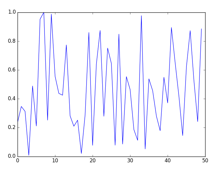
PyObject <matplotlib.lines.Line2D object at 0x0000000026314198>Apart from the printed value presented earlier, a plot window will open as shown in the following figure:
- Now, exit Julia and run the script in non-interactive mode from the OS shell:
$ julia display.jl
 sum(r) = 23.134209483707394
 1×50 LinearAlgebra.Transpose{Float64,Array{Float64,1}}:
 0.236033 0.346517 0.312707 0.00790928 0.488613 0.210968 0.951916 0.999905 0.251662 0.986666 0.555751 0.437108 0.424718 0.773223 0.28119 0.209472 0.251379 0.0203749 0.287702 0.859512 0.0769509 0.640396 0.873544 0.278582 0.751313 0.644883 0.0778264 0.848185 0.0856352
 0.553206 0.46335 0.185821 0.111981 0.976312 0.0516146 0.53803 0.455692 0.279395 0.178246 0.548983 0.370971 0.894166 0.648054 0.417039 0.144566 0.622403 0.872334 0.524975 0.241591 0.884837[0.236033 0.346517 0.312707 0.00790928 0.488613 0.210968 0.951916 0.999905 0.251662 0.986666 0.555751 0.437108 0.424718 0.773223 0.28119 0.209472 0.251379 0.0203749 0.287702 0.859512 0.0769509 0.640396 0.873544 0.278582 0.751313 0.644883 0.0778264 0.848185 0.0856352 0.553206 0.46335 0.185821 0.111981 0.976312 0.0516146 0.53803 0.455692 0.279395 0.178246 0.548983 0.370971 0.894166 0.648054 0.417039 0.144566 0.622403 0.872334 0.524975 0.241591 0.884837]
In this case, nothing is plotted. Additionally, observe that the display function, in this case, produced a different output than in interactive mode and no newline was inserted after the result (so the output of the print function is visually merged).
- Now, add
show()afterplot(r)in thedisplay.jlfile and name itdisplay2.jl:
using PyPlot, Random

function f()
    Random.seed!(1)
    r = rand(50)
    @show sum(r)
    display(transpose(r))
    print(transpose(r))
    plot(r)
    show()
end

f()
- Run the updated file as a script:
$ julia display2.jlThis time the plot is shown and Julia is suspended until the plot dialog is closed.
In Julia, the display function is aware of the context in which it is called. This means that depending on what context is passed to this function, you may obtain a different result. For instance, an image passed to the display in the Julia console usually opens a new window with a plot, but in Jupyter Notebook it might embed it in a notebook. Similarly, many objects in the Julia console are displayed as plain text but in Jupyter Notebook they are converted to a nicely formatted HTML. In short, display(x) typically uses the richest supported multimedia output for x in a given context, with plain text stdout output as a fallback.
In particular, the display function is used by default in the Julia console when a command is executed, for example:
julia> transpose(1:100)
1×100 LinearAlgebra.Transpose{Int64,UnitRange{Int64}}:
 1 2 3 4 5 6 7 8 9 10 11 … 93 94 95 96 97 98 99 100
In this case, the output is adjusted to the size of the Terminal. However, as we saw in the previous example if display is run in a script in non-interactive mode, no adjustment of the output to the size of the device is performed.
An additional issue that is commonly required in practice is suppressing the display of an expression value in the Julia console. This is easily achieved by adding ; at the end of the command, for example:
julia> rand(100, 100);

julia>
And nothing is printed (otherwise, the screen would be flooded by a large matrix).
Finally, in the script in this recipe, we were able to examine the use of the @show macro, which is useful for debugging, as it prints the expression along with its value.
At the end of this recipe, we observed that the PyPlot package can alter its behavior based on whether it is run in interactive mode or not. Each custom package might have similar specific conditions for handling output to a variety of devices. Being aware of this, it is best to consult the documentation relating to a given package to understand the defaults.
If you are developing your own code that needs to be sensitive to the Julia mode (REPL or script) in which it is invoked, there is a handy isinteractive function. This function allows you to dynamically check the Julia interpreter mode at runtime.
An in-depth explanation of how display management in Julia works is given at https://docs.julialang.org/en/v1.0/manual/types/#man-custom-pretty-printing-1.
In the Defining your own types - linked list recipe in Chapter 6, Metaprogramming and Advanced Typing, we explain how to specify custom printing for user-defined types.
Julia has a built-in package manager that allows you to fully control the combination of packages that your project can use.
In this recipe, we explain the fundamentals of how to manage packages in a default (global) project. In the Managing project dependencies recipe in Chapter 8, Julia Workflow, we discuss how you can customize which packages you use in your local project repositories.
In this recipe, we will use the Julia command line. Make sure that your computer is connected to the internet.
Note
In the GitHub repository for this recipe, you will find the commands.txt file that contains the presented sequence of shell and Julia commands.
Now open your favorite terminal to execute the commands.
Here is a list of steps to be followed:
- Go to the Julia command line:
julia>- Press ] to switch to the package manager mode:
(v1.0) pkg>- We can check the initial status of packages using the
statuscommand:
(v1.0) pkg> status
    Status `~/.julia/environments/v1.0/Project.toml`
We can see that we currently have a clean environment with no additional packages installed.
- To add the
BenchmarkToolspackage, use theaddcommand:
(v1.0) pkg> add BenchmarkTools
   Cloning default registries into /home/ubuntu/.julia/registries
   Cloning registry General from "https://github.com/JuliaRegistries/General.git"
  Updating registry at `~/.julia/registries/General`
  Updating git-repo `https://github.com/JuliaRegistries/General.git`
 Resolving package versions...
 Installed BenchmarkTools ─ v0.4.1
 Installed JSON ─────────── v0.19.0
  Updating `~/.julia/environments/v1.0/Project.toml`
  [6e4b80f9] + BenchmarkTools v0.4.1
  Updating `~/.julia/environments/v1.0/Manifest.toml`
  [6e4b80f9] + BenchmarkTools v0.4.1
  [682c06a0] + JSON v0.19.0
  [2a0f44e3] + Base64
  [ade2ca70] + Dates
  [8ba89e20] + Distributed
  [b77e0a4c] + InteractiveUtils
  [76f85450] + LibGit2
  [8f399da3] + Libdl
  [37e2e46d] + LinearAlgebra
  [56ddb016] + Logging
  [d6f4376e] + Markdown
  [a63ad114] + Mmap
  [44cfe95a] + Pkg
  [de0858da] + Printf
  [3fa0cd96] + REPL
  [9a3f8284] + Random
  [ea8e919c] + SHA
  [9e88b42a] + Serialization
  [6462fe0b] + Sockets
  [2f01184e] + SparseArrays
  [10745b16] + Statistics
  [8dfed614] + Test
  [cf7118a7] + UUIDs
[4ec0a83e] + Unicode- Now, use the
statuscommand to see the versions of your installed packages:
(v1.0) pkg> status
    Status `~/.julia/environments/v1.0/Project.toml`
  [6e4b80f9] BenchmarkTools v0.4.1
Notice that only the BenchmarkTools package is visible, although more packages have been installed by Julia. They reside in the package repository but are not visible to the user unless explicitly installed. Those packages are dependencies of the BenchmarkTools package (directly or via recursive dependency).
- After installing a package, we precompile the installed packages:
(v1.0) pkg> precompile
Precompiling project...
Precompiling BenchmarkTools
[ Info: Precompiling BenchmarkTools [6e4b80f9-dd63-53aa-95a3-0cdb28fa8baf]- Exit the package manager mode by pressing the Backspace key:
(v1.0) pkg>

julia>
- Now, we can check that the package can be loaded and used:
julia> using BenchmarkTools

julia> @btime rand()
  4.487 ns (0 allocations: 0 bytes)
0.07253910317708079
- Finally, install the
BSONpackage versionv0.2.0(this is not the latest version of this package, as as of writing of the book the currently released version isv0.2.1). Switch to the PackageManager mode by pressing]and then type:
(v1.0) pkg> add BSON@v0.2.0
[output is omitted]
Now you have version 0.2.0 of the BSON package installed
- Often you want to keep the version of some package fixed to avoid its update by the Julia Package Manager, when its new version is released. You can achieve it with the
pincommand as follows
(v1.0) pkg> pin BSON
[output is omitted]- If you decide that you want to allow the Julia Package Manager to update some package that was pinned you can do it using the
freecommand:
(v1.0) pkg> free BSON
[output is omitted]
The process of installing a specified version of some package (step 9 of the recipe) and pinning it (step 10) might be useful for you when you will need to install the exact versions of the packages that we use in this book, as in the future new releases of the packages might introduce breaking changes. The full list of packages used in this book along with their required versions is given in the To get the most out of this book section in the Preface of this book.
For each environment, Julia keeps information about the required packages and their versions in the Project.tomlandManifest.tomlfiles. For the global default environment, they are placed in the ~/.julia/environments/v1.0/folder. The first file contains a list of installed packages along with their UUIDs (see https://en.wikipedia.org/wiki/Universally_unique_identifier or https://www.itu.int/ITU-T/studygroups/com17/oid.html). The second file describes detailed dependencies of the project with exact versions of the packages used.
In this recipe, we have only made use of the basic commands of the package manager. In most cases, this is all a regular user needs to know. There are many more commands available, which you can find using the help command in package manager mode. Some of the potentially useful commands are as follows:
add: installs the indicated packagerm: removes the indicated packageup: updates the indicated package to a different versiondevelop: Clones the full package repository locally for development (useful in circumstances such as when wanting to use the latestmasterversion of the package)up: Updates packages in the manifest (be warned that updating packages in your project might lead to incompatibilities with old code, so use this with caution)build: Runs the build script for packages (useful as sometimes installing packages fails to correctly build them, for example, due to external dependencies that have to be configured)pin: Pins the version of packages (ensures that a given package version is not changed by using other commands)free: Undoes apin,develop, or stops tracking a repository
All the commands we have described are also available programmatically using functions from the Pkg.jl package. For instance, running Pkg.add("BenchmarkTools") would install the package the same way as writing add BenchmarkTools in package manager mode in the Julia console. In order to use those functions, you have to load the Pkg package using using Pkg first.
In addition, it is important to know that many packages are preinstalled with Julia and thus do not require installation and can be directly loaded with the using command. Here is a selection of some of the more important ones, along with a brief description of their functionality:
Dates: Works with date and time featuresDelimitedFiles: Basic loading and writing of delimited filesDistributed: MultiprocessingLinearAlgebra: Various operations on matricesLogging: Support for loggingPkg: Package managerRandom: Random number generationSerialization: Support for serialization/deserialization of Julia objectsSparseArrays: Support for non-dense arraysStatistics: Basic statistical functionsTest: Support for writing unit tests
Extensive coverage of these packages is given in the standard library section of the Julia manual, which can be accessed at https://docs.julialang.org/en/v1.0/.
The true power of the Julia package manager is realized when you need to have different versions of packages for your different projects on the same machine. In the Managing project dependencies recipe in Chapter 8, Julia Workflow, we discuss how you can achieve this.
Jupyter Notebook is a de facto standard for exploratory data science analysis. In this recipe, we show how to configure Jupyter with Julia.
Before installing Jupyter Notebook, perform the following steps:
Prepare a Linux machine with Julia installed (you can follow the instructions in the Installing Julia from binaries recipe).
Open a Julia console.
Install the
IJuliapackage. Press]in the Julia REPL to go to the Julia package manager and execute theadd IJuliacommand:
(v1.0) pkg> add IJuliaOnce IJulia is installed, there are two options for running Jupyter Notebook:
Running Jupyter Notebook from within the Julia console
Running Jupyter Notebook from bash
Simply start the Julia console and run the following commands:
julia> using IJulia

julia> notebook()
A web browser window will open with Jupyter, where you can start to work with Julia. In order to stop the Jupyter Notebook server, go back to the console and press Ctrl + C.
In order to run Jupyter Notebook outside of Julia, firstly make sure that you have installed IJulia (see the Getting ready section). Once IJulia is installed, perform the following steps:
- Execute the shell command (this assumes thatyou used the default setting for the Julia
packagesfolder; in particular thehsaaNpart of the path below might be different; in such case please look-up the correct path in the~/.julia/packages/Conda/folder):
$ ~/.julia/packages/Conda/hsaaN/deps/usr/bin/jupyter notebook
Please note that the preceding command in Windows will look different:
C:\> %userprofile%\.julia\packages\Conda\hsaaN\deps\usr\Scripts\jupyter-notebook- Look for console output similar to what is shown here:
Copy/paste this URL into your browser when you connect for the first time,
to login with a token:
http://localhost:8888/?token=b86b66b81a62d4be1ae34e7d6bd006a8ba5cb937e74b99cf- Paste the link (in the preceding output marked with bold font) into your browser's address bar.
Jupyter Notebook runs a local web server on port 8888. Once it is started, you can simply connect to it via a web browser. It is also possible to run such environments on a different machine than that used to access the notebook—please check the Jupyter in the cloud recipe for more details.
Please note that for some packages, Julia installation might have conflicts with Windows security settings and thus prevent installation. In particular, IE Enhanced Security Configuration should be turned off (the default setting on Windows Server environments is on). In order to turn it off, open Server Manager and click Local Server, which is located on the left. In the right column, you will see the option IE Enhanced Security Configuration. Click on it to turn it off.
Another possible problem can be with the installation of IJulia, since it sometimes conflicts with an existing Python installation due to IJulia attempting to fetch and install a minimal Python environment itself. In such cases, if you get an error, run the following:
ENV["JUPYTER"] ="[path to your jupyter program]"
using Pkg
Pkg.build("IJulia")
You will have to manually find the[path to your jupyter program]. For example, on my Windows system with Anaconda installed, the path will be"C:\\Program Files\\Anaconda\\Scripts\\jupyter-notebook.exe".Note that we need to use two backslashes of the Julia string to represent a single backslash in a path. If you have provided a proper path, the build should finish successfully.
The most recent documentation can be found on IJulia's website(https://github.com/JuliaLang/IJulia.jl). It is worth checking, as some details of the process described earlier may change.
JupyterLab is a new, extended version of Jupyter Notebook. Before installing it, make sure that you have successfully completed the Configuring Julia in Jupyter Notebook tutorial. Running JupyterLab requires Python to be installed. We strongly recommend Python Anaconda as the standard execution environment.
The configuration of JupyterLab requires having IJulia configured on your system:
Prepare a Linux or Windows machine with Julia installed.
- Follow the Configuring Julia in Jupyter Notebook tutorial and install
IJulia.
Note
In the GitHub repository for this recipe, you will find the commands.txt file that contains the presented sequence of shell and Julia commands.
By default, Julia does not include JupyterLab. However, it is possible to add JupyterLab by using the Conda.jl package. We will show, step-by-step, how to add JupyterLab to a Julia installation and run it from bash:
- Press the ] key to go to the Julia package manager and install the
Conda.jlpackage:
(v1.0) pkg> add Conda- Use
Condato add JupyterLab to Julia's installation:
julia> using Conda

julia> Conda.add("jupyterlab")
- Once JupyterLab is installed, exit Julia and run it from the command line:
$ ~/.julia/packages/Conda/hsaaN/deps/usr/bin/jupyter lab- Please note that the preceding command in Windows will look different:
C:\>%userprofile%\.julia\packages\Conda\hsaaN\deps\usr
\Scripts\jupyter-lab- If the preceding command did not automatically start the web browser, do it manually andlook for console output similar to this:
Copy/paste this URL into your browser when you connect for the first time,
to login with a token:
http://localhost:8888/?token=b86b66b81a62d4be1ae34e7d6bd006a8ba5cb937e74b99cf- Paste the link (in the preceding output marked with bold font) into your browser's address bar.
Once you have followed the preceding steps, you should see in the browser a screen similar to the one shown here (please note that since Python is installed with IJulia.jl, it is also available alongside Julia):
JupyterLab is an extension of Jupyter Notebook and hence it works in a very similar fashion. JupyterLab runs a local web server on port8888 (the same port that would have been used by Jupyter Notebook). Once it is started, you can simply connect to it via a web browser. It is also possible to run such environments on a separate machine. Please check the Configuring Julia with Jupyter Notebook headless cloud environments recipe for more details (that recipe is valid for both Jupyter Notebook and JupyterLab).
Yet another option is to use JupyterLab from a completely external Anaconda installation. Since the installation process differs for Linux and Windows, we present both versions.
In order to install JupyterLab on Linux, perform the following steps:
- Go to the Anaconda for Linux download website (https://www.anaconda.com/download/#linux) and find the current download link for the 64-bit Python 3 version (usually it can be done in a web browser by right-clicking the
Downloadbutton and selectingCopy link location). - Download Anaconda Python. Please note that depending on the time when you perform the installation, the exact link might look different—new Anaconda versions are being released frequently:
$ wget https://repo.anaconda.com/archive/Anaconda3-5.3.0-Linux-x86_64.sh- Run the Anaconda installer:
$ sudo bash Anaconda3-5.3.0-Linux-x86_64.sh- Now, you can launch JupyterLab (we assume that you have selected the standard install locations):
$ /home/ubuntu/anaconda3/bin/jupyter lab- If the preceding command did not automatically start the web browser, do it manually andlook for console output similar to this:
[I 11:07:55.625 LabApp] The Jupyter Notebook is running at:
[I 11:07:55.625 LabApp] http://localhost:8888/?token=c3756ac2013d780af16b0401d67ab017c5e4a17cc9bc7924
[I 11:07:55.625 LabApp] Use Control-C to stop this server and shut down all kernels (twice to skip confirmation).
[W 11:07:55.625 LabApp] No web browser found: could not locate runnable browser.- Paste the link (in the preceding log marked with bold font) your browser's address bar.
Please note that if you follow the preceding steps (including the installation of the IJulia.jlpackage), once you open the JupyterLab welcome screen, you should see Python 3 as well as Julia Notebook execution kernels.
In the following steps, we describe to run JupyterLab with Anaconda on Windows:
- Go to the Anaconda for Windows download website (https://www.anaconda.com/download/#windows) and find the current download link for the 64-bit Python 3 version. Download the
*.exeinstallation file to your computer. - Run the installer. Here, we assume that you are installing it to the default folder, which on Windows is
C:\ProgramData\Anaconda3\.
- Once Anaconda 3 is installed, simply run
jupyter-lab.exe:
C:\> C:\ProgramData\Anaconda3\Scripts\jupyter-lab.exe- If the preceding command did not automatically start the web browser, do it manually andlook for console output similar to this:
Copy/paste this URL into your browser when you connect for the first time,  to login with a token:
http://localhost:8888/?token=7f211507e188ecfc22e2858b195c8de915c7c221f012ee86- Paste the link (in the preceding log marked with bold font) into your browser's address bar.
Please note that if you follow the preceding steps (including the installation of the IJulia.jl package), once you open the JupyterLab welcome screen, you should see Python 3 as well as Julia Notebook execution kernels.
The JupyterLab project is developing rapidly, so it is worth checking the latest news on the project's website(https://github.com/jupyterlab/jupyterlab).
In this recipe, we show how to configure Jupyter (both JupyterLab and Jupyter Notebook) for use in Terminal-only environments on a Linux platform (that is, environments that do not provide any graphical desktop interface). For these remote environments, running Jupyter Notebook is trickier. For illustrative purposes, we will use the AWS Cloud.
Before you start, you need to have a Linux machine with IJulia and either Jupyter Notebook or JupyterLab installed:
Prepare a Linux machine (for example, an AWS EC2 instance) with Julia installed, and Jupyter Notebook or JupyterLab (you can follow the instructions in the previous recipes).
Make sure that you can open an SSH connection to your Linux machine. If this is an instance of Linux on the AWS Cloud, you can follow the instructions given at https://docs.aws.amazon.com/AWSEC2/latest/UserGuide/AccessingInstancesLinux.html.In particular, you need to know the server's address, login name (in the examples we use
ubuntu, which is the default username on Ubuntu Linux), and have the private key file (in the examples, we name itkeyname.pem, and the user's password could be used instead of the key file).
Note
Please note that for Windows 10, there is no default SSH client. Hence, this recipe has been tested with the SSH client included with Git for Windows tools, available at https://git-scm.com/download/win/. Once Git for Windows is installed, the SSH executable by default can be found at C:\Program Files\Git\usr\bin\ssh.exe.Please note that on *ux environments (for example, Linux, OS X) the key file, keyfile.pem, which is used for connection should be readable only to the local user. If you just downloaded it from AWS, you need to execute the$ chmod 400 keyfile.pem command before running the ssh command to open the SSH connection.
A general scenario for working with Jupyter Notebook/JupyterLab on a remote machine consists of the following three steps:
- Set up the SSH tunnel on port
8888 - Start JupyterLab on the remote machine
- Find the link in the launch log and copy it to the browser on the local machine
We discuss each step in detail and consider alternative configurations for Jupyter Notebook and JupyterLab:
- Connect to the Linux machine from your desktop computer (local machine). While opening the SSH connection, set up a tunnel on port
8888. In place of[enter_hostname_here], provide the appropriate hostname (for example, in the AWS Cloud, the hostname could look like this:ec2-18-188-4-172.us-east-2.compute.amazonaws.com):
$ ssh -i path/to/keyfile.pem -L8888:127.0.0.1:8888 ubuntu@[enter_hostname_here]
- Once the connection has been set up, run your Jupyter Notebook or JupyterLab on the remote machine. Execute the command shown (this assumes that the
IJuliapackage is installed on your machine along with instructions from the previous recipes and you used the default setting for the Juliapackagesfolder):
$ ~/.julia/packages/Conda/hsaaN/deps/usr/bin/jupyter labPlease note that the Windows version of the preceding command is the following:
C:\> %userprofile%\.julia\packages\Conda\hsaaN\deps\usr\Scripts\jupyter-labYou can also use either Jupyter Lab or Jupyter Notebook command versions (see the instructions from the previous recipe).
Note
Please note that, depending on your Julia and Anaconda configuration, the executable jupyter file could be in a different location. On Linux environments, you can search for it with the $ find ~/ -name "jupyter" command. This assumes the search is run in your local home folder.
- Look for console output similar to this:
Copy/paste this URL into your browser when you connect for the first time,to login with a token:
http://localhost:8888/?token=b86b66b81a62d4be1ae34e7d6bd006a8ba5cb937e74b99cf- Paste the link marked with bold to your browser on your local machine (not the remote server).
If you have properly configured the SSH tunnel, you should see Jupyter Notebook/JupyterLab running on the remote server in the browser on the local machine. Please note that the environment will be available for only as long as the SSH connection is open. If you close the SSH connection, you will lose access to your Jupyter Notebook or JupyterLab.
Using Jupyter Notebook via the internet requires setting up an SSH tunnel to the server. This is the option we present in this tutorial. Please note that on a local network, you can connect directly to the server without SSH tunneling.
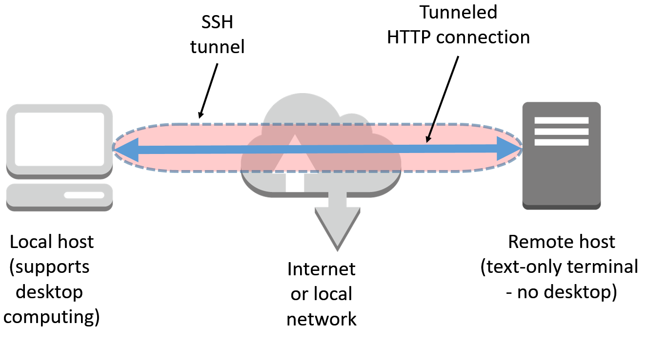
In the preceding scenario, the command-line argument-L 8888:127.0.0.1:8888 tells ssh to open a secure tunnel over SSH from your machine to port 8888 on the target machine in the cloud (as shown in the following diagram):
Yet another option for running IJulia on a text-only Terminal remote machine is to use a detached mode for the Jupyter environment. However, in order to obtain access to Jupyter Notebook, a token key is required. Please see the following example:
julia> usingIJulia

julia> notebook(detached=true)

julia> run(`$(IJulia.notebook_cmd[1]) notebook list`)
Currently running servers:
http://localhost:8888/?token=2bb8421e3bba78c8c551a8af1f22460bb4bb3fdc5a0986bb
Now, you can simply copy and paste the preceding link into your web browser.
More information on SSH tunneling can be found at https://www.ssh.com/ssh/tunneling/example.