There are different approaches to make computers solve tasks. One of them is to define an explicit algorithm, and another one is to use implicit strategies based on mathematical and statistical methods. Machine Learning (ML) is one of the implicit methods that uses mathematical and statistical approaches to solve tasks. It is an actively growing discipline, and a lot of scientists and researchers find it to be one of the best ways to move forward toward systems acting as human-level artificial intelligence (AI).

In general, ML approaches have the idea of searching patterns in a given dataset as their basis. Consider a recommendation system for a news feed, which provides the user with a personalized feed based on their previous activity or preferences. The software gathers information about the type of news article the user reads and calculates some statistics. For example, it could be the frequency of some topics appearing in a set of news articles. Then, it performs some predictive analytics, identifies general patterns, and uses them to populate the user's news feed. Such systems periodically track a user's activity, and update the dataset and calculate new trends for recommendations.

There are many areas where ML has started to play an important role. It is used for solving enterprise business tasks as well as for scientific researches. In customer relationship management (CRM) systems, ML models are used to analyze sales team activity, to help them to process the most important requests first. ML models are used in business intelligence (BI) and analytics to find essential data points. Human resource (HR) departments use ML models to analyze their employees' characteristics in order to identify the most effective ones and use this information when searching applicants for open positions.

A fast-growing direction of research is self-driving cars, and deep learning neural networks are used extensively in this area. They are used in computer vision systems for object identification as well as for navigation and steering systems, which are necessary for car driving.

Another popular use of ML systems is electronic personal assistants, such as Siri from Apple or Alexa from Amazon. Such products also use deep learning models to analyze natural speech or written text to process users' requests and make a natural response in a relevant context. Such requests can activate music players with preferred songs, as well as update a user's personal schedule or book flight tickets.

This chapter describes what ML is and which tasks can be solved with ML, and discusses different approaches used in ML. It aims to show the minimally required math to start implementing ML algorithms. It also covers how to perform basic linear algebra operations in libraries such as Eigen, xtensor, Shark-ML, Shogun, and Dlib, and also explains the linear regression task as an example.

The following topics will be covered in this chapter:

• Understanding the fundamentals of ML
• An overview of linear algebra
• An overview of a linear regression example

There are different approaches to create and train ML models. In this section, we show what these approaches are and how they differ. Apart from the approach we use to create a ML model, there are also parameters that manage how this model behaves in the training and evaluation processes. Model parameters can be divided into two distinct groups, which should be configured in different ways. The last crucial part of the ML process is a technique that we use to train a model. Usually, the training technique uses some numerical optimization algorithm that finds the minimal value of a target function. In ML, the target function is usually called a loss function and is used for penalizing the training algorithm when it makes errors. We discuss these concepts more precisely in the following sections.

We can divide ML approaches into two techniques, as follows:

• Supervised learning is an approach based on the use of labeled data. Labeled data is a set of known data samples with corresponding known target outputs. Such a kind of data is used to build a model that can predict future outputs.
• Unsupervised learning is an approach that does not require labeled data and can search hidden patterns and structures in an arbitrary kind of data.

Let's have a look at each of the techniques in detail.

Supervised ML algorithms usually take a limited set of labeled data and build models that can make reasonable predictions for new data. We can split supervised learning algorithms into two main parts, classification and regression techniques, described as follows:

• Classification models predict some finite and distinct types of categories—this could be a label that identifies if an email is spam or not, or whether an image contains a human face or not. Classification models are applied in speech and text recognition, object identification on images, credit scoring, and others. Typical algorithms for creating classification models are Support Vector Machine (SVM), decision tree approaches, k-nearest neighbors (KNN), logistic regression, Naive Bayes, and neural networks. The following chapters describe the details of some of these algorithms.
• Regression models predict continuous responses such as changes in temperature or values of currency exchange rates. Regression models are applied in algorithmic trading, forecasting of electricity load, revenue prediction, and others. Creating a regression model usually makes sense if the output of the given labeled data is real numbers. Typical algorithms for creating regression models are linear and multivariate regressions, polynomial regression models, and stepwise regressions. We can use decision tree techniques and neural networks to create regression models too. The following chapters describe the details of some of these algorithms.

Unsupervised learning algorithms do not use labeled datasets. They create models that use intrinsic relations in data to find hidden patterns that they can use for making predictions. The most well-known unsupervised learning technique is clustering. Clustering involves dividing a given set of data in a limited number of groups according to some intrinsic properties of data items. Clustering is applied in market researches, different types of exploratory analysis, deoxyribonucleic acid (DNA) analysis, image segmentation, and object detection. Typical algorithms for creating models for performing clustering are k-means, k-medoids, Gaussian mixture models, hierarchical clustering, and hidden Markov models. Some of these algorithms are explained in the following chapters of this book.

We can interpret ML models as functions that take different types of parameters. Such functions provide outputs for given inputs based on the values of these parameters. Developers can configure the behavior of ML models for solving problems by adjusting model parameters. Training a ML model can usually be treated as a process of searching the best combination of its parameters. We can split the ML model's parameters into two types. The first type consists of parameters internal to the model, and we can estimate their values from the training (input) data. The second type consists of parameters external to the model, and we cannot estimate their values from training data. Parameters that are external to the model are usually called hyperparameters.

Internal parameters have the following characteristics:

• They are necessary for making predictions.
• They define the quality of the model on the given problem.
• We can learn them from training data.
• Usually, they are a part of the model.

If the model contains a fixed number of internal parameters, it is called parametric. Otherwise, we can classify it as non-parametric.

Examples of internal parameters are as follows:

• Weights of artificial neural networks (ANNs)
• Support vector values for SVM models
• Polynomial coefficients for linear regression or logistic regression

On the other hand, hyperparameters have the following characteristics:

• They are used to configure algorithms that estimate model parameters.
• The practitioner usually specifies them.
• Their estimation is often based on using heuristics.
• They are specific to a concrete modeling problem.

It is hard to know the best values for a model's hyperparameters for a specific problem. Also, practitioners usually need to perform additional research on how to tune required hyperparameters so that a model or a training algorithm behaves in the best way. Practitioners use rules of thumb, copying values from similar projects, as well as special techniques such as grid search for hyperparameter estimation.

Examples of hyperparameters are as follows:

• C and sigma parameters used in the SVM algorithm for a classification quality configuration
• The learning rate parameter that is used in the neural network training process to configure algorithm convergence
• The k value that is used in the KNN algorithm to configure the number of neighbors

Model parameter estimation usually uses some optimization algorithm. The speed and quality of the resulting model can significantly depend on the optimization algorithm chosen. Research on optimization algorithms is a popular topic in industry, as well as in academia. ML often uses optimization techniques and algorithms based on the optimization of a loss function. A function that evaluates how well a model predicts on the data is called a loss function. If predictions are very different from the target outputs, the loss function will return a value that can be interpreted as a bad one, usually a large number. In such a way, the loss function penalizes an optimization algorithm when it moves in the wrong direction. So, the general idea is to minimize the value of the loss function to reduce penalties. There is no one universal loss function for optimization algorithms. Different factors determine how to choose a loss function. Examples of such factors are as follows:

• Specifics of the given problem—for example, if it is a regression or a classification model
• Ease of calculating derivatives
• Percentage of outliers in the dataset

In ML, the term optimizer is used to define an algorithm that connects a loss function and a technique for updating model parameters in response to the values of the loss function. So, optimizers tune ML models to predict target values for new data in the most accurate way by fitting model parameters. There are many optimizers: Gradient Descent, Adagrad, RMSProp, Adam, and others. Moreover, developing new optimizers is an active area of research. For example, there is the ML and Optimization research group at Microsoft (located in Redmond) whose research areas include combinatorial optimization, convex and non-convex optimization, and their application in ML and AI. Other companies in the industry also have similar research groups; there are many publications from Facebook Research, Amazon Research, and OpenAI groups.

The concepts of linear algebra are essential for understanding the theory behind ML because they help us understand how ML algorithms work under the hood. Also, most ML algorithm definitions use linear algebra terms.

Linear algebra is not only a handy mathematical instrument, but also the concepts of linear algebra can be very efficiently implemented with modern computer architectures. The rise of ML, and especially deep learning, began after significant performance improvement of the modern Graphics Processing Unit (GPU). GPUs were initially designed to work with linear algebra concepts and massive parallel computations used in computer games. After that, special libraries were created to work with general linear algebra concepts. Examples of libraries that implement basic linear algebra routines are Cuda and OpenCL, and one example of a specialized linear algebra library is cuBLAS. Moreover, it became more common to use general-purpose graphics processing units (GPGPUs) because these turn the computational power of a modern GPU into a powerful general-purpose computing resource.

Also, Central Processing Units (CPUs) have instruction sets specially designed for simultaneous numerical computations. Such computations are called vectorized, and common vectorized instruction sets are AVx, SSE, and MMx. There is also a term Single Instruction Multiple Data (SIMD) for these instruction sets. Many numeric linear algebra libraries, such as Eigen, xtensor, VienaCL, and others, use them to improve computational performance.

Linear algebra is a big area. It is the section of algebra that studies objects of a linear nature: vector (or linear) spaces, linear representations, and systems of linear equations. The main tools used in linear algebra are determinants, matrices, conjugation, and tensor calculus.

To understand ML algorithms, we only need a small set of linear algebra concepts. However, to do researches on new ML algorithms, a practitioner should have a deep understanding of linear algebra and calculus.

The following list contains the most valuable linear algebra concepts for understanding ML algorithms:

• Scalar: This is a single number.
• Vector: This is an array of ordered numbers. Each element has a distinct index. Notation for vectors is a bold lowercase typeface for names and an italic typeface with a subscript for elements, as shown in the following example:

• Matrix: This is a two-dimensional array of numbers. Each element has a distinct pair of indices. Notation for matrices is a bold uppercase typeface for names and an italic but not bold typeface with a comma-separated list of indices in subscript for elements, as shown in the following example:

• Tensor: This is an array of numbers arranged in a multidimensional regular grid, and represents generalizations of matrices. It is like a multidimensional matrix. For example, tensor A with dimensions 2 x 2 x 2 can look like this:

Linear algebra libraries and ML frameworks usually use the concept of a tensor instead of a matrix because they implement general algorithms, and a matrix is just a special case of a tensor with two dimensions. Also, we can consider a vector as a matrix of size n x 1.

The most common operations used for programming linear algebra algorithms are the following ones:

• Element-wise operations: These are performed in an element-wise manner on vectors, matrices, or tensors of the same size. The resulting elements will be the result of operations on corresponding input elements, as shown here:

The following example shows the element-wise summation:

• Dot product: There are two types of multiplications for tensor and matrices in linear algebra—one is just element-wise, and the second is the dot product. The dot product deals with two equal-length series of numbers and returns a single number. This operation applied on matrices or tensors requires that the matrix or tensor A has the same number of columns as the number of rows in the matrix or tensor B. The following example shows the dot-product operation in the case when A is an n x m matrix and B is an m x p matrix:

• Transposing: The transposing of a matrix is an operation that flips the matrix over its diagonal, which leads to the flipping of the column and row indices of the matrix, resulting in the creation of a new matrix. In general, it is swapping matrix rows with columns. The following example shows how transposing works:

• Norm: This operation calculates the size of the vector; the result of this is a non-negative real number. The norm formula is as follows:

The generic name of this type of norm is norm for . Usually, we use more concrete norms such as an norm with p = 2, which is known as the Euclidean norm, and we can interpret it as the Euclidean distance between points. Another widely used norm is the squared norm, whose calculation formula is . The squared norm is more suitable for mathematical and computational operations than the norm. Each partial derivative of the squared norm depends only on the corresponding element of x, in comparison to the partial derivatives of the norm which depends on the entire vector; this property plays a vital role in optimization algorithms. Another widely used norm operation is the norm with p=1, which is commonly used in ML when we care about the difference between zero and nonzero elements.

• Inverting: The inverse matrix is such a matrix that , where I is an identity matrix. The identity matrix is a matrix that does not change any vector when we multiply that vector by that matrix.

We considered the main linear algebra concepts as well as operations on them. Using this math apparatus, we can define and program many ML algorithms. For example, we can use tensors and matrices to define training datasets for training, and scalars can be used as different types of coefficients. We can use element-wise operations to perform arithmetic operations with a whole dataset (a matrix or a tensor). For example, we can use element-wise multiplication to scale a dataset. We usually use transposing to change a view of a vector or matrix to make them suitable for the dot-product operation. The dot product is usually used to apply a linear function with weights expressed as matrix coefficients to a vector; for example, this vector can be a training sample. Also, dot-product operations are used to update model parameters expressed as matrix or tensor coefficients according to an algorithm.

The norm operation is often used in formulas for loss functions because it naturally expresses the distance concept and can measure the difference between target and predicted values. The inverse matrix is a crucial concept for the analytical solving of linear equations systems. Such systems often appear in different optimization problems. However, calculating the inverse matrix is very computationally expensive.

We can represent tensor objects in computer memory in different ways. The most obvious method is a simple linear array in computer memory (random-access memory, or RAM). However, the linear array is also the most computationally effective data structure for modern CPUs. There are two standard practices to organize tensors with a linear array in memory: row-major ordering and column-major ordering. In row-major ordering, we place consecutive elements of a row in linear order one after the other, and each row is also placed after the end of the previous one. In column-major ordering, we do the same but with the column elements. Data layouts have a significant impact on computational performance because the speed of traversing an array relies on modern CPU architectures that work with sequential data more efficiently than with non-sequential data. CPU caching effects are the reasons for such behavior. Also, a contiguous data layout makes it possible to use SIMD vectorized instructions that work with sequential data more efficiently, and we can use them as a type of parallel processing.

Different libraries, even in the same programming language, can use different ordering. For example, Eigen uses column-major ordering, but PyTorch uses row-major ordering. So, developers should be aware of internal tensor representation in libraries they use, and also take care of this when performing data loading or implementing algorithms from scratch.

Consider the following matrix:

Then, in the row-major data layout, members of the matrix will have the following layout in memory:

In the case of the column-major data layout, order layout will be the next, as shown here:

Consider some C++ linear algebra APIs (short for Application Program Interface), and look at how we can use them for creating linear algebra primitives and perform algebra operations with them.

Eigen is a general-purpose linear algebra C++ library. In Eigen, all matrices and vectors are objects of the Matrix template class, and the vector is a specialization of the matrix type, with either one row or one column. Tensor objects are not presented in official APIs but exist as submodules.

We can define the type for a matrix with known dimensions and floating-point data type like this:

typedef Eigen::Matrix<float, 3, 3> MyMatrix33f;

We can define a vector in the following way:

typedef Eigen::Matrix<float, 3, 1> MyVector3f;

Eigen already has a lot of predefined types for vector and matrix objects—for example, Eigen::Matrix3f (floating-point 3x3 matrix type) or Eigen::RowVector2f (floating-point 1 x 2 vector type). Also, Eigen is not limited to matrices whose dimensions we know at compile time. We can define matrix types that will take the number of rows or columns at initialization during runtime. To define such types, we can use a special type variable for the Matrix class template argument named Eigen::Dynamic. For example, to define a matrix of doubles with dynamic dimensions, we can use the following definition:

typedef Eigen::Matrix<double, Eigen::Dynamic, Eigen::Dynamic> MyMatrix;

Objects initialized from the types we defined will look like this:

MyMatrix33f a;
MyVector3f v;
MyMatrix m(10,15);

To put some values into these objects, we can use several approaches. We can use special predefined initialization functions, as follows:

a = MyMatrix33f::Zero(); // fill matrix elements with zeros
a = MyMatrix33f::Identity(); // fill matrix as Identity matrix
v = MyVector3f::Random(); // fill matrix elements with random values

We can use the comma-initializer syntax, as follows:

a << 1,2,3,
     4,5,6,
     7,8,9;

This code construction initializes the matrix values in the following way:

We can use direct element access to set or change matrix coefficients. The following code sample shows how to use the () operator for such an operation:

a(0,0) = 3;

We can use the object of the Map type to wrap an existent C++ array or vector in the Matrix type object. This kind of mapping object will use memory and values from the underlying object, and will not allocate the additional memory and copy the values. The following snippet shows how to use the Map type:

int data[] = {1,2,3,4};
Eigen::Map<Eigen::RowVectorxi> v(data,4);
std::vector<float> data = {1,2,3,4,5,6,7,8,9};
Eigen::Map<MyMatrix33f> a(data.data());

We can use initialized matrix objects in mathematical operations. Matrix and vector arithmetic operations in the Eigen library are offered either through overloads of standard C++ arithmetic operators such as +, -, *, or through methods such as dot() and cross(). The following code sample shows how to express general math operations in Eigen:

using namespace Eigen;   
auto a = Matrix2d::Random();
auto b = Matrix2d::Random();
auto result = a + b;
result = a.array() * b.array(); // element wise multiplication
result = a.array() / b.array();
a += b;
result = a * b; // matrix multiplication
//Also it’s possible to use scalars:
a = b.array() * 4;

Notice that in Eigen, arithmetic operators such as operator+ do not perform any computation by themselves. These operators return an expression object, which describes what computation to perform. The actual computation happens later when the whole expression is evaluated, typically in the operator= arithmetic operator. It can lead to some strange behaviors, primarily if a developer uses the auto keyword too frequently.

Sometimes, we need to perform operations only on a part of the matrix. For this purpose, Eigen provides the block method, which takes four parameters: i,j,p,q. These parameters are the block size p,q and the starting point i,j. The following code shows how to use this method:

Eigen::Matrixxf m(4,4);
Eigen::Matrix2f b = m.block(1,1,2,2); // copying the middle part of matrix
m.block(1,1,2,2) *= 4; // change values in original matrix

There are two more methods to access rows and columns by index, which are also a type of block operation. The following snippet shows how to use the col and the row methods:

m.row(1).array() += 3;
m.col(2).array() /= 4;

Another important feature of linear algebra libraries is broadcasting, and Eigen supports this with the colwise and rowwise methods. Broadcasting can be interpreted as a matrix by replicating it in one direction. Take a look at the following example of how to add a vector to each column of the matrix:

Eigen::Matrixxf mat(2,4);
Eigen::Vectorxf v(2); // column vector
mat.colwise() += v;

This operation has the following result: .

The xtensor library is a C++ library for numerical analysis with multidimensional array expressions. Containers of xtensor are inspired by NumPy, the Python array programming library. ML algorithms are mainly described using Python and NumPy, so this library can make it easier to move them to C++. The following container classes implement multidimensional arrays in the xtensor library.

The xarray type is a dynamically sized multidimensional array, as shown in the following code snippet:

std::vector<size_t> shape = { 3, 2, 4 };
xt::xarray<double, xt::layout_type::row_major> a(shape);

The xtensor type is a multidimensional array whose dimensions are fixed at compilation time. Exact dimension values can be configured in the initialization step, as shown in the following code snippet:

std::array<size_t, 3> shape = { 3, 2, 4 };
xt::xtensor<double, 3> a(shape);

The xtensor_fixed type is a multidimensional array with a dimension shape fixed at compile time, as shown in the following code snippet:

xt::xtensor_fixed<double, xt::xshape<3, 2, 4>> a;

The xtensor library also implements arithmetic operators with expression template techniques such as Eigen (this is a common approach for math libraries implemented in C++). So, the computation happens lazily, and the actual result is calculated when the whole expression is evaluated. The container definitions are also expressions. There is also a function to force an expression evaluation named xt::eval in the xtensor library.

There are different kinds of container initialization in the xtensor library.
Initialization of xtensor arrays can be done with C++ initializer lists, as follows:

        xt::xarray<double> arr1{{1.0, 2.0, 3.0},
                                {2.0, 5.0, 7.0},
                                {2.0, 5.0, 7.0}}; // initialize a 3x3 array

The xtensor library also has builder functions for special tensor types. The following snippet shows some of them:

std::vector<uint64_t> shape = {2, 2};
xt::ones(shape);
xt::zero(shape);
xt::eye(shape); //matrix with ones on the diagonal

Also, we can map existing C++ arrays into the xtensor container with the xt::adapt function. This function returns the object that uses the memory and values from the underlying object, as shown in the following code snippet:

std::vector<float> data{1,2,3,4};
std::vector<size_t> shape{2,2};
auto data_x = xt::adapt(data, shape);

We can use direct access to container elements, with the () operator, to set or change tensor values, as shown in the following code snippet:

std::vector<size_t> shape = {3, 2, 4};
xt::xarray<float> a = xt::ones<float>(shape);
a(2,1,3) = 3.14f;

The xtensor library implements linear algebra arithmetic operations through overloads of standard C++ arithmetic operators such as +, - and *. To use other operations such as dot-product operations, we have to link an application with the library named xtensor-blas. These operators are declared in the xt::linalg namespace.

The following code shows the use of arithmetic operations with the xtensor library:

auto a = xt::random::rand<double>({2,2});
auto b = xt::random::rand<double>({2,2});
auto c = a + b;
a -= b;
c = xt::linalg::dot(a,b);
c = a + 5;

To get partial access to the xtensor containers, we can use the xt::view function. The following sample shows how this function works:

xt::xarray<int> a{{1,  2,  3,  4},
                  {5,  6,  7,  8}
                  {9,  10, 11, 12}
                  {13, 14, 15, 16}};
auto b = xt::view(a, xt::range(1, 3), xt::range(1, 3));

This operation takes a rectangular block from the tensor, which looks like this:

The xtensor library implements automatic broadcasting in most cases. When the operation involves two arrays of different dimensions, it transmits the array with the smaller dimension across the leading dimension of the other array, so we can directly add a vector to a matrix. The following code sample shows how easy it is:

auto m = xt::random::rand<double>({2,2});
auto v = xt::random::rand<double>({2,1});
auto c = m + v;

Shark-ML is a C++ ML library with rich functionality. It also provides an API for linear algebra routines.

There are four container classes for representing matrices and vectors in the Shark-ML library. Notice that the linear algebra functionality is declared in the remora namespace instead of the shark namespace, which is used for other routines.

The following code sample shows container classes that exist in the Shark-ML library, wherein the vector type is a dynamically sized array:

remora::vector<double> b(100, 1.0); // vector of size 100 and filled with 1.0

The compressed_vector type is a sparse array storing values in a compressed format.

The matrix type is a dynamically sized dense matrix, as shown in the following code snippet:

remora::matrix<double> C(2, 2); // 2x2 matrix

The compressed_matrix type is a sparse matrix storing values in a compressed format.

There are two main types of container initialization in the Shark-ML library.

We can initialize a container object with the constructor that takes the initializer list. The following code sample shows this:

remora::matrix<float> m_ones{{1, 1}, {1, 1}}; // 2x2 matrix

The second option is to wrap the existing C++ array into the container object and reuse its memory and values. The following code sample shows how to use the same array for the initialization of matrix and vector objects:

float data[]= {1,2,3,4};
remora::matrix<float> m(data, 2, 2);
remora::vector<float> v(data, 4);

Also, we can initialize values with direct access to the container elements, with the () operator. The following code sample shows how to set a value for matrix and vector objects:

remora::matrix<float> m(data, 2, 2);
m(0,0) = 3.14f;
remora::vector<float> v(data, 4);
v(0) = 3.14f;

The Shark-ML library implements linear algebra arithmetic operations through overloads of standard C++ arithmetic operators such as +, - and *. Some other operations such as the dot product are implemented as standalone functions.

The following code sample shows how to use arithmetic operations in the Shark-ML library:

remora::matrix<float> a(data, 2, 2);
remora::matrix<float> b(data, 2, 2);
auto c = a + b;
a -= b;
c = remora::prod(a,b);
c = a%b; // also dot product operation
c = a + 5;

We can use the following functions for partial access to the Shark ML containers:

• subrange (x,i,j): This function returns a sub-vector of x with the elements xi,…, xj−1.
• subrange (A,i,j,k,l): This function returns a sub-matrix of A with elements indicated by i,…, j−1 and k, …, l−1.
• row (A,k): This function returns the k^th row of A as a vector proxy.
• column (A,k): This function returns the k^th column of A as a vector proxy.
• rows (A,k,l): This function returns the rows k,…,l−1 of A as a matrix proxy.
• columns (A,k,l): This function returns the columns k,…, l−1 of A as a matrix proxy.

There is no broadcasting implementation in the Shark-ML library. Limited support of broadcasting exists only in the form of reduction functions (the set of functions that calculate one numeric value for a whole matrix or vector). There are two functions—the as_rows() and as_columns() function—that allow reduction operations to be performed independently on matrix rows or columns respectively. We can pass the result of these functions to any of the reduction functions. The following code sample shows how to perform summation reduction:

remora::matrix<float> m{{1, 2, 3, 4}, {5, 6, 7, 8}};
auto cols = remora::as_columns(m);
remora::sum(cols)

A different way to work with columns and rows independently is the use of partial access functions. The following code sample shows how to add the same vector to each of the matrix columns:

remora::vector<float> v{10, 10};
// Update matrix rows
for (size_t i = 0; i < m.size2(); ++i) {         
   remora::column(m, i) += v;
}

Dlib is a modern C++ toolkit containing ML algorithms and tools for creating computer vision software in C++. Most of the linear algebra tools in Dlib deal with dense matrices. However, there is also limited support for working with sparse matrices and vectors. In particular, the Dlib tools represent sparse vectors using the containers from the C++ standard template library (STL).

There are two main container types in Dlib to work with linear algebra: the matrix and the vector classes. Matrix operations in Dlib are implemented using the expression templates technique, which allows them to eliminate the temporary matrix objects that would usually be returned from expressions such as M = A+B+C+D.

We can create a matrix sized at compile time in the following way, by specifying dimensions as template arguments:

Dlib::matrix<double,3,1> y;

Alternatively, we can create dynamically sized matrix objects. In such a case, we pass the matrix dimensions to the constructor, as shown in the following code snippet:

Dlib::matrix<double> m(3,3);

Later, we can change the size of this matrix, with the following method:

m.set_size(6,6);

We can initialize matrix values with a comma operator, as shown in the following code snippet:

m = 54.2,  7.4, 12.1,
    1,     2,    3,
    5.9,   0.05, 1;

As in the previous libraries, we can wrap an existing C++ array to the matrix object, as shown in the following code snippet:

double data[] = {1,2,3,4,5,6};
auto a = Dlib::mat(data, 2,3); // create matrix with size 2x3

Also, we can access matrix elements with the () operator to modify or get a particular value, as shown in the following code snippet:

m(1,2) = 3;

The Dlib library has a set of predefined functions to initialize a matrix with values such as identity matrix, 1s, or random values, as illustrated in the following code snippet:

auto a = Dlib::identity_matrix<double>(3);
auto b = Dlib::ones_matrix<double>(3,4);
auto c = Dlib::randm(3,4); // matrix with random values with size 3x3

Most linear algebra arithmetic operations in the Dlib library are implemented through overloads of standard C++ arithmetic operators such as +, -, *. Other complex operations are provided by the library as standalone functions.

The following example shows the use of arithmetic operations in the Dlib library:

auto c = a + b;
auto e = a * b; // real matrix multiplication
auto d  = Dlib::pointwise_multiply(a, b); // element wise multiplication
a += 5;
auto t = Dlib::trans(a); // transpose matrix

To work with partial access to matrices, Dlib provides a set of special functions. The following code sample shows how to use some of them:

a = Dlib::rowm(b,0); // takes first row of matrix
a = Dlib::rowm(b,Dlib::range(0,1));//takes first two rows
a = Dlib::colm(b,0); // takes first column
a = Dlib::subm(b, range(1,2), range(1,2)); // takes a rectangular part from center
Dlib::set_subm(b,range(0,1), range(0,1)) = 7; // initialize part of the matrix
Dlib::set_subm(b,range(0,1), range(0,1)) += 7; // add a value to the part of the matrix

Broadcasting in the Dlib library can be modeled with set_rowm(), set_colm(), and set_subm() functions that give modifier objects for a particular matrix row, column, or a rectangular part of the original matrix. Objects returned from these functions support all set or arithmetic operations. The following code snippet shows how to add a vector to the columns:

Dlib::matrix<float, 2,1> x;
Dlib::matrix<float, 2,3> m;
Dlib::set_colm(b,Dlib::range(0,1)) += x;

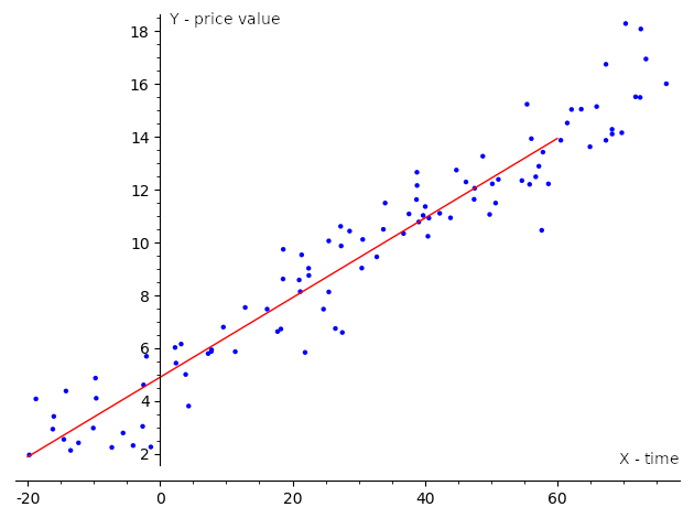
Consider an example of the real-world supervised ML algorithm called linear regression. In general, linear regression is an approach for modeling a target value (dependent value) based on an explanatory value (independent value). This method is used for forecasting and finding relationships between values. We can classify regression methods by the number of inputs (independent variables) and the type of relationship between the inputs and outputs (dependent variables).

Simple linear regression is the case where the number of independent variables is 1, and there is a linear relationship between the independent (x) and dependent (y) variable.

Linear regression is widely used in different areas, such as scientific research, where it can describe relationships between variables, as well as in applications within industry, such as a revenue prediction. For example, it can estimate a trend line that represents the long-term movement in the stock price time-series data. It tells whether the interest value of in a specific dataset has increased or decreased over the given period, as illustrated in the following screenshot:

If we have one input variable (independent variable) and one output variable (dependent variable) the regression is called simple, and we use the term simple linear regression for it. With multiple independent variables, we call this multiple linear regression or multivariable linear regression. Usually, when we are dealing with real-world problems, we have a lot of independent variables, so we model such problems with multiple regression models. Multiple regression models have a universal definition that covers other types, so even simple linear regression is often defined using the multiple regression definition.

Assume that we have a dataset, , so that we can express the linear relation between y and x with mathematical formula in the following way:

Here, p is the dimension of the independent variable, and T denotes the transpose, so that is the inner product between vectors and β. Also, we can rewrite the previous expression in matrix notation, as follows:

,,,

The preceding matrix notation can be explained as follows:

• y: This is a vector of observed target values.
• x: This is a matrix of row-vectors, , which are known as explanatory or independent values.
• ß: This is a (p+1) dimensional parameters vector.
• ε: This is called an error term or noise. This variable captures all other factors that influence the y dependent variable other than the regressors.

When we are considering simple linear regression, p is equal to 1, and the equation will look like this:

The goal of the linear regression task is to find parameter vectors that satisfy the previous equation. Usually, there is no exact solution to such a system of linear equations, so the task is to estimate parameters that satisfy these equations with some assumptions. One of the most popular estimation approaches is one based on the principle of least squares: minimizing the sum of the squares of the differences between the observed dependent variable in the given dataset and those predicted by the linear function. This is called the ordinary least squares (OLS) estimator. So, the task can be formulated with the following formula:

In the preceding formula, the objective function S is given by the following matrix notation:

This minimization problem has a unique solution, in the case that the p columns of the x matrix are linearly independent. We can get this solution by solving the normal equation, as follows:

Linear algebra libraries can solve such equations directly with an analytical approach, but it has one significant disadvantage—computational cost. In the case of large dimensions of y and x, requirements for computer memory amount and computational time are too big to solve real-world tasks.

So, usually, this minimization task is solved with iterative approaches. Gradient descent (GD) is an example of such an algorithm. GD is a technique based on the observation that if the function is defined and is differentiable in a neighborhood of a point , then decreases fastest when it goes in the direction of the negative gradient of S at the point .

We can change our objective function to a form more suitable for an iterative approach. We can use the mean squared error (MSE) function, which measures the difference between the estimator and the estimated value, as illustrated here:

In the case of the multiple regression, we take partial derivatives for this function for each of x components, as follows:

So, in the case of the linear regression, we take the following derivatives:

The whole algorithm has the following description:

1. Initialize β with zeros.
2. Define a value for the learning rate parameter that controls how much we are adjusting parameters during the learning procedure.
3. Calculate the following values of β:

4. Repeat steps 1-3 for a number of times or until the MSE value reaches a reasonable amount.

The previously described algorithm is one of the simplest supervised ML algorithms. We described it with the linear algebra concepts we introduced earlier in the chapter. Later, it became more evident that almost all ML algorithms use linear algebra under the hood. The following samples show the higher-level API in different linear algebra libraries for solving the linear regression task, and we provide them to show how libraries can simplify the complicated math used underneath. We will give the details of the APIs used in these samples in the following chapters.

There are several iterative methods for solving problems of the form in the Eigen library. The LeastSquaresConjugateGradient class is one of them, which allows us to solve linear regression problems with the conjugate gradient algorithm. The ConjugateGradient algorithm can converge more quickly to the function's minimum than regular GD but requires that matrix A is positively defined to guarantee numerical stability. The LeastSquaresConjugateGradient class has two main settings: the maximum number of iterations and a tolerance threshold value that is used as a stopping criteria as an upper bound to the relative residual error, as illustrated in the following code block:

typedef float DType;
using Matrix = Eigen::Matrix<DType, Eigen::Dynamic, Eigen::Dynamic>;
int n = 10000;
Matrix x(n,1);
Matrix y(n,1);
Eigen::LeastSquaresConjugateGradient<Matrix> gd;
gd.setMaxIterations(1000);
gd.setTolerance(0.001) ;
gd.compute(x);
auto b = dg.solve(y);

For new x inputs, we can predict new y values with matrices operations, as follows:

Eigen::Matrixxf new_x(5, 2);
new_x << 1, 1, 1, 2, 1, 3, 1, 4, 1, 5;
auto new_y = new_x.array().rowwise() * b.transpose().array();

Also, we can calculate parameter's b vector (the linear regression task solution) by solving the normal equation directly, as follows:

auto b = (x.transpose() * x).ldlt().solve(x.transpose() * y);

Shogun is an open source ML library that provides a wide range of unified ML algorithms. The Shogun library has the CLinearRidgeRegression class for solving simple linear regression problems. This class solves problems with standard Cholesky matrix decomposition in a noniterative way, as illustrated in the following code block:

auto x = some<CDenseFeatures<float64_t>>(x_values);
auto y= some<CRegressionLabels>(y_values); // real-valued labels
float64_t tau_regularization = 0.0001;
auto lr = some<CLinearRidgeRegression>(tau_regularization, nullptr, nullptr); // regression model with regularization
lr->set_labels(y);
r->train(x)

For new x inputs, we can predict new y values in the following way:

auto new_x = some<CDenseFeatures<float64_t>>(new_x_values);
auto y_predict = lr->apply_regression(new_x);

Also, we can get the calculated parameters (the linear regression task solution) vector, as follows:

auto weights = lr->get_w();

Moreover, we can calculate the value of MSE, as follows:

auto y_predict = lr->apply_regression(x);
auto eval = some<CMeanSquaredError>();
auto mse = eval->evaluate(y_predict , y);

The Shark-ML library provides the LinearModel class for representing linear regression problems. There are two trainer classes for this kind of model: the LinearRegression class, which provides analytical solutions, and the LinearSAGTrainer class, which provides a stochastic average gradient iterative method, as illustrated in the following code block:

using namespace shark;
using namespace std;
Data<RealVector> x;
Data<RealVector> y;
RegressionDataset data(x, y);
LinearModel<> model;

LinearRegression trainer;
trainer.train(model, data);

We can get the calculated parameters (the linear regression task solution) vector by running the following code:

auto b = model.parameterVector();

For new x inputs, we can predict new y values in the following way:

Data<RealVector> new_x;
Data<RealVector> prediction = model(new_x);

Also, we can calculate the value of squared error, as follows:

SquaredLoss<> loss;
auto se = loss(y, prediction)

The Dlib library provides the krr_trainer class, which can get the template argument of the linear_kernel type to solve linear regression tasks. This class implements direct analytical solving for this type of problem with the kernel ridge regression algorithm, as illustrated in the following code block:

std::vector<matrix<double>> x;
std::vector<float> y;
krr_trainer<KernelType> trainer;
trainer.set_kernel(KernelType());
decision_function<KernelType> df = trainer.train(x, y);

For new x inputs, we can predict new y values in the following way:

std::vector<matrix<double>> new_x;
for (auto& v : x) {
    auto prediction = df(v);
    std::cout << prediction << std::endl;
}

In this chapter, we learned what ML is, how it differs from other computer algorithms, and how it became so popular. We also became familiar with the necessary mathematical background required to begin to work with ML algorithms. We looked at software libraries that provide APIs for linear algebra, and also implemented our first ML algorithm—linear regression.

There are other linear algebra libraries for C++. Moreover, the popular deep learning frameworks use their own implementations of linear algebra libraries. For example, the MXNet framework is based on the mshadow library, and the PyTorch framework is based on the ATen library. Some of these libraries can use GPU or special CPU instructions for speeding up calculations. Such features do not usually change the API but require some additional library initialization settings or explicit object conversion to different backends such as CPUs or GPUs.

In the next two chapters, we will learn more about available software tools that are necessary to implement more complicated algorithms, and we will also learn more theoretical background on how to manage ML algorithms.

• Basic Linear Algebra for Deep Learning: https://towardsdatascience.com/linear-algebra-for-deep-learning-f21d7e7d7f23
• Deep Learning - An MIT Press book: https://www.deeplearningbook.org/contents/linear_algebra.html
• What is Machine Learning?: https://www.mathworks.com/discovery/machine-learning.html
• The Eigen library documentation: http://eigen.tuxfamily.org
• The xtensor library documentation: https://xtensor.readthedocs.io/en/latest/
• The Dlib library documentation: http://dlib.net/
• The Shark-ML library documentation: http://image.diku.dk/shark/
• The Shogun library documentation: http://www.shogun-toolbox.org/