In this book, we are going to learn about data analysis from the perspective of the Haskell
programming language. The goal of this book is to take you from being a beginner in math
and statistics, to the point that you feel comfortable working with large-scale datasets.
Now, the prerequisites for this book are that you know a little bit of the Haskell
programming language, and also a little bit of math and statistics. From there, we can start
you on your journey of becoming a data analyst.

In this chapter, we are going to cover descriptive statistics. Descriptive statistics are used to summarize a collection of values into one or two values. We begin with learning about the Haskell Text.CSV library. In later sections, we will cover in increasing difficulty the range, mean, median, and mode; you've probably heard of some of these descriptive statistics before, as they're quite common. We will be using the IHaskell environment on the Jupyter Notebook system.

The topics that we are going to cover are as follows:

• The CSV library—working with CSV files
• Data ranges
• Data mean and standard deviation
• Data median
• Data mode

In this section, we're going to cover the basics of the CSV library and how to work with CSV files. To do this, we will be taking a closer look at the structure of a CSV file; how to install the Text.CSV Haskell library; and how to retrieve data from a CSV file from within Haskell.

Now to begin, we need a CSV file. So, I'm going to tab over to my Haskell environment, which is just a Debian Linux virtual machine running on my computer, and I'm going to go to the website at retrosheet.org. This is a website for baseball statistics, and we are going to use them to demonstrate the CSV library. Find the link for Data Downloads and click Game Logs, as follows:

Now, scroll down just a little bit and you should see game logs for every single season, going all the way back to 1871. For now, I would like to stick with the most recent complete season, which is 2015:

So, go ahead and click the 2015 link. We will have the option to download a ZIP file, so go ahead and click OK. Now, I'm going to tab over to my Terminal:

Let's go into the Downloads folder, and if we hit ls, we see that there's our ZIP file. Let's unzip that file and see what we have. Let's open up GL2015.TXT. This is a CSV file, and will display something like the following:

A CSV file is a file of comma-separated values. So, you'll see that we have a file divided up, where each line in this file is a record, and each record represents a single game of baseball in the 2015 season; and inside every single record is a listing of values, separated by a comma. So, the very first game in this dataset is a game between the St. Louis Cardinals—that's SLN—and the Chicago Cubs—that's CHN—and this game took place on March 5th 2015. The final score of this first game was 3-0, and every line in this file is a different game.

Now, CSV isn't a standard, but there are a few properties of a CSV file which I consider to be safe. Consider the following as my suggestions. A CSV file should keep one record per line. The first line should be a description of each column. In a future section, I'm going to tell you that we need to remove the header line; and you'll see that this particular file doesn't have this header line. I still like to see the description line for each column of values. If a field in a record includes a comma, then that field should be surrounded by double quote marks. Now we don't see an example of this—at least, not on this first line—but we do see examples of many values having quote marks surrounding the file, such as the very first value in the file, the date:

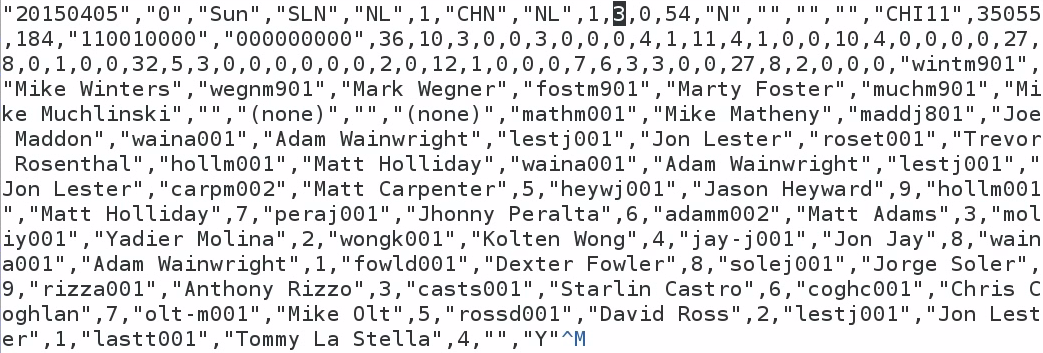
In a CSV file, if a field is surrounded by quote marks, then it is optional, unless it has a comma inside that value. While we're here, I would like to make a note of the tenth column in this file, which contains the number 3 on this particular row. This represents the away-team score in every single record of this file. Make a note that our first value on the tenth column is a 3—we're going to come back to that later on.

Our next task is installing the Text.CSV library; we do this using the Cabal tool, which connects with the Hackage repository and downloads the Text.CSV library:

The command that we use to start the install, shown in the first line of the preceding screenshot, is cabal install csv. It takes a moment to download the file, but it should download and install the Text.CSV library in our home folder. Now, let me describe what I currently have in my home folder:

I like to create a directory for my code called Code; and inside here, I have a directory called HaskellDataAnalysis. And inside HaskellDataAnalysis, I have two directories, called analysis and data. In the analysis folder, I would like to store my notebooks. In the data folder, I would like to store my datasets.

That way, I can keep a clear distinction between analysis files and data files. That means I need to move the data file, just downloaded, into my data folder. So, copy GL2015.TXT from our Downloads folder into our data folder. If I do an ls on my data folder, I'll see that I've got my file. Now, I'm going to go into my analysis folder, which currently contains nothing, and I'm going to start the Jupyter Notebook as follows:

Type in jupyter notebook, which will start a web server on your computer. You can use your web browser in order to interact with Haskell:

The address for the Jupyter Notebook is the localhost, on port 8888. Now I'm going to create a new Haskell notebook. To do this, I click on the New drop-down button on the right side of the screen, and I find Haskell:

Let's begin by renaming our notebook Baseball, because we're going to be looking at baseball statistics:

I need to import the Text.CSV file that we just installed. Now, if your cursor is sitting in a text field and you hit Enter, you'll just be making that text field larger, as shown in the following screenshot. Instead, in order to submit expressions to the Jupyter environment, you have to hit hit Shift + Enter on the keyboard:

So, now that we've imported Text.CSV, let's create our Baseball dataset and parse the dataset. The command for this is parseCSVFromFile, after which we pass in the location of our text file:

Great. If you didn't get a File Not Found error at this point, then that means you have successfully parsed the data from the CSV file. Now, let's explore the type of baseball data. To do this, we enter type and baseball, which is what we just created, and we see that we have either a parsing error or a CSV file:

I've already done this, so I know that there aren't any parsing errors in our CSV file, but if there were, they would be represented by ParseError. So I can promise you that if you've gotten this far, you know that we have a working CSV file. Now, I'll be honest: I don't know why the CSV library does this, but the last element in every CSV data is a single empty list, and I call this empty list the "empty row". What I would like to do is to create a quick function, called noEmptyRows, that removes any row of data that doesn't have at least two pieces of information in it:

So, if we have a parsing error, we're just going to return back an empty list, and if we actually have data, we're going to filter out any row that does not have at least two pieces of information in that row. Now, let's apply our noEmptyRows to our Baseball dataset:

I'm going to call this baseballList. Then we can do a quick check to see the length of the baseballList, and we should have 2,429 rows representing 2,429 games played in the 2015 season.

Now let's look at the type of baseballList, and we see that we have a list of fields:

Now, you may be asking yourself: What's a field? We can explore a field using info, and doing so will bring up a window from the bottom of the screen:

It says type Field = String, and it's defined in this Text.CSV library. So, just remember that a field is just a string.

Now, because every value is a field that is also a string, that means that if I do math on strings, it's going to produce an error message, as shown in the following screenshot:

So what I need to do is to parse that information from a string to something else that I can use, such as an int or a double, and I do that with the read command. Let's look at an example:

So if I say read "1", it will be parsed as an Integer, or, if I say read "1.5", then it will be parsed as a Double.

So, armed with this knowledge of parsing data from strings, we can parse a whole column of data. Create a readIndex function, and let's say that, in our case, each value is a cell:

So for each cell in our dataset, we're going to pass in our original Baseball dataset—this is an Either; and we're going to say that we need an Int index position in our list; and we are going to return a list of cells. This requires two arguments: the csv, and the index position that we need. And we are going to map over each record, and we're going to read whatever exists at the specified index position. We also need the noEmptyRows function that we discussed earlier.

Now, if you recall earlier, I said that the away-team scores in our CSV file exist on column 10, and because Haskell is a zero-based index file, that means we need to pass in index 9 to our readIndex function:

Here, we parse this list that's returned as a list of integers, and we are returned a listing of every single away-team score in Major League Baseball. The very first element in our list is a 3, because that is the first record of the file.

In this section, you learned about the structure of a CSV file, how to install the Text.CSV library, and how to pull a little bit of information out of that CSV file using the CSV library. In the next section, we're going to discuss how to create our own module for descriptive statistics, and how to write a function for the range of a dataset.

We begin with the data range descriptive statistic. This will be the easiest descriptive statistic that we cover in this chapter. This is basically grabbing the maximum and minimum of a range of values. So, in this section, we're going to be taking a look at using the maximum and minimum functions in order to find the range of a dataset, and we're going to be combining those functions into a single function that returns a tuple of values. And finally, we're going to compute the range of our away-team runs using the function that we prototyped previously.

Let's go to our Haskell notebook in the Jupyter environment. In the last section, we pulled a listing of all the away-team scores for each game in the 2015 season of Major League Baseball. If you're rejoining this section after a break, you may have to find the Kernel and Restart & Run All feature inside the Notebook system:

Now we get a warning message, saying that this will clear all of our variables, but that's okay because all of the variables are going to be rebuilt by the notebook.

The last thing we did was pass in index 9 to get the away scores. Now, let's store this in a variable called awayRuns:

In order to find the range of this dataset, we're going to utilize two functions, maximum awayRuns and minimum awayRuns:

We see that the maximum number of runs scored by any away team in the 2015 season was 21, and we see that the minimum was 0. Let's take a moment to examine the type signatures of the maximum and minimum functions:

They both take a list of values and return a single value, and the values are bound by the Ord type. With that knowledge, we're going to create a function, called range, that takes a value and returns a tuple of values bound by the Ord type. Let's go. Our quick function should probably look like this:

So, we've called this a range, and we have bound our values by the Ord type. We have also accepted a range of values, and returned our tuple of values. And then, we entered range xs, which will extend from minimum xs to maximum xs. Now, let's test this function.

Testing range awayRuns, we see that we get a range of 0 to 21:

Now, what if we pass an empty list, or what if we just passed a list of one value? These are some things that we didn't consider in this function that I just wrote, so let's explore that briefly:

We see that we get an error message—Prelude.minimum: empty list—and that's because our data was passed to the minimum function. It saw that we had an empty list and it threw an error. What we really ought to do is to package our return in a Maybe so that we could potentially return nothing, and adjust this for cases where we have empty list:

The preceding screenshot shows our improved range function. We use a little bit of pattern matching in order to adjust to some of the conditions that we should be looking for in a proper range function. So, we still have a list of values that are bound by the Ord type, but now, we are packaging our return inside of a Maybe. That way, we can adjust the circumstances in which an empty list is passed, such as by returning nothing. If we have a single value, we can just return that value twice, and not even have to worry with the minimum and maximum. But if we get anything else, we can utilize our minimum and maximum functions. This means that we can produce the range of an empty list (range []), range [1], and our full range awayRuns:

Great. So, this improved function is going to be our prototype for the remaining descriptive statistics in this book. We're going to be adjusting accordingly based on the inputs given, and returning Nothing in cases where no results should be given. In the next section, we're going to be discussing how to compute the mean of a dataset.

The next descriptive statistics covered will be the mean, also called the average, and standard deviation. In this section, we will use the sum and length functions to compose the mean of a dataset. We'll also explore the sum and length functions; compose our mean function; and then use that mean function in order to compose a standard deviation function. Finally, we're going to compute the mean and standard deviation of the 2015 away-team runs using our function.

The mean is a summary statistic that gives you a rough idea of the middle values of the dataset, while not truly being the middle of a dataset:

The mean is trivial to calculate and thus it is frequently used, and it is the sum of that dataset divided by the number of values in that dataset.

We will also discuss sample standard deviation, which is the mean distance from the mean and a measure of a dataset spread. The approach that we will be using is known as the sample standard deviation. I have presented the function here for your reference:

Now, let's go over to our Linux environment. We left off last section discussing the range of a dataset. Let's add a new import now, Data.Maybe, as follows:

Here, we have added a library. Each time we add libraries, we will restart and rerun all, and it's okay to do this. It will take a moment, and will reload all of our variables.

In order to compute the mean of a dataset, we add up all the values and divide this value by the length of those values. So, in order to find the sum of all the values in a list, we use sum on the awayRuns variable, and we also need to find the length of the awayRuns variable:

There were 10,091 runs scored in the 2015 season by the away team, and 2,429 games played in that season. We divide the first number by the second, and we get our average; but we need to explore the type of the sum and the length functions:

We can see that the sum takes a list of values and returns a value, and the sum inputs and the outputs are bound by the Num type, whereas the inputs on length aren't bound by anything, and they always return an int. The division operator in Haskell doesn't work with int, so what we need to do is to convert the values returned by sum and length to something that we can work with:

So the function we have used for this is realToFrac, where we pass sum of the away runs divided by fromIntegral, which takes the length of the away runs. So, our average is 4.15 runs per game scored by away teams in the 2015 season. We use this information in order to compose our mean function:

Much like our range function, we have a return type of a double that's been packaged into a Maybe, and we have a list of values that are bound on the Real type. Our function uses pattern matching in order to handle the variety of inputs and outputs that we will likely receive, much like we did with the range function in the last section. So, if we have a list of no values, we return Nothing. Now, it's best that we return Nothing, and not 0, because 0 could be interpreted as a mean of a dataset. If we have a single value, then we're just going to return that value bundled in Just, and if we have a list, then we're actually going to implement the sum and length functions that we described earlier. So, let's test this out:

As we can see, if we get the mean of an empty list, we should get Nothing; if we get mean of a single value, we should get that value converted to a double; and if we have mean of a true list, we should get our average, which in our case is 4.15.

Now, any function that uses our mean function is going to have to interpret the value inside of Maybe, so in order to do that, we use a function called fromJust. Now, let's write the code for the standard deviation, as follows:

Much like the mean function we wrote earlier, we have our inputs bound by a Real type; and we will be returning a Double packaged to the Maybe. And for historical reasons, we will call this function stdev. Statistical spreadsheet software and statistical packages will call this particular function stdev, which is a recreation of the formula that we saw at the beginning of this section, which produces the sample standard deviation. It's important to note that the sample standard deviation requires at least two values in order to compute a spread. You can't very well compute a spread with one value, and so we need to use pattern matching in order to detect that, thus if we have an empty list, we return Nothing. If we have a list of just one item, we still return Nothing. After that, we have actually implemented the formula necessary for the sample standard deviation. Let's do a few tests:

So, the standard deviation of a blank list is Nothing; the standard deviation of a single item is still Nothing; and the standard deviation of our awayRuns is 3.12. With this information, we are going to take our average which is 4.15, and we will subtract it with 3.12 and we will also add 3.12 to it:

We can say that one standard deviation range of our away-team runs for the 2015 season is 1.03 runs to 7.27 runs; and that gives us a good idea of where the majority of the scores were for away teams in the 2015 season. So, in this section, we looked at the mean and the standard deviations of a dataset. We implemented the functions; we discussed the sum and the length functions necessary for those functions; and then we did a few examples of how we could find the mean and standard deviation with the functions that we had prototyped. In the next section, we will be discussing the median of a dataset.

The median of a dataset is the true middle value of the values sorted. Now, if there isn't a single middle value, such as if there's an even number of elements in the list, then we take the average of the two values closest to the sorted middle. In this video, we're going to discuss the algorithm for computing the median of a dataset, and we're going to take the traditional approach of sorting the values first and then selecting the values we need in order to compute the median. We're going to be testing the circumstances under which the median function should behave, and then we're going to compute the median of our 2015 away-team runs using our prototyped function.

In the last section, we were discussing the mean and standard deviation of runs; and we found that one standard deviation range was 1.03 to 7.27. Now, for this topic, we will have to add yet another import, and we're going to import Data.List, as this is where we find the sort function:

Now, as usual, we will restart and rerun all so that everything is properly loaded for our notebook. Next, let's create a couple of quick lists, just to demonstrate the sort function:

So, here we have oddList, which contains the comma-separated values "3,4,1,2,5", and we have an evenList, which contains "6,5,4,3,2,1". We can use the sort function to sort these lists as follows:

This was pretty straightforward—the sort function is found in the Data.List library. If we wish to find the middle value of a list, we need to find the length of the list and then divide by 2:

So, we have used the length of oddList and then divided it by 2, and it produces 2. Now we can sort that odd list and pull out the second element:

After sorting, we got 3; and 3 is the median of our odd list. And for an odd list, that's all you have to do.

Whenever we pass an even list, you should notice that we get the index position that appears after the median. So, if we divide the length of evenList by 2, we will get 3 as shown in the following screenshot:

The index position for 3 in our sorted even list will be 4, which is not the median. So, we need to take the two values that are closest to the middle, which in this case it will be index 3; and then the index position before that, which is 2; and then add those together and divide by 2. So, the formula is as follows:

As we can see that our median is 3.5, which is the true median of our even list. There are algorithms for finding the median that do not require the full sort of values, such as you can use the quickselect algorithm to quickly find the median sorted value in a list. But for our purposes, we're going to stay with the traditional sort the values first approach. We're going to prototype a median function utilizing the approach that we've outlined here. We're going to go over a few quick examples of what should happen whenever median is called:

So, here is our median prototyped function. Notice that we are bounding our inputs based on type Real, and we are packaging once again a Double inside of a Maybe. We're using Double because, you know, there's the possibility that even though we have a full list of integers, we still need to return a double because we have an even number of integers. If we have a median of no items, then we return Nothing. Other than that, we are going to have the possibility of an odd list; then we will return the middleValue. Otherwise, we are going to return the middleEven. After that, we have outlined all of the different circumstances. So, let's test out a few examples:

Whenever we return the median of an empty list, we get Nothing. Likewise, if we get the median of oddList, we should get back 3. Notice it's been converted to a double. And if we do the median of an evenList, we get 3.5. And to outline again, we have our middleValue, which is just the middleIndex; and we have the beforeMiddleValue, which is middleIndex - 1. And the middleEven is simply those two values divided by 2; and that's all there really is to it. We're using the odd function in order to look for an odd number of elements; otherwise, we're going to use the even approach.

So, using sort, we built a function for finding the median of a list. This was a long function, and we described it in detail. Finally, we need to use the median function, which we have prototyped already, in order to find the away runs:

We found that the middle sorted value of array runs in the 2015 season is 4. In our next section, we are going to discuss what's probably the simplest of the descriptive statistics to discuss, and that is the mode, but it turns out to be one of the more difficult to compute.

The mode is the value in a list which appears the most frequently. In this section, we are going to discuss an algorithm for finding the mode. We will first try to understand how the mode of a list can be solved using Run-Length Encoding (RLE). We will then break that problem of RLE into parts, and then write the code for our function. Finally, we will use RLE in order to find the mode of a dataset, and then we're going to compute the mode of our 2015 away runs dataset.

To find the mode, we will have to do yet another import. We need to go back up to the very top of the Baseball dataset and import Data.Ord:

We need this for a function that we'll use later on in this section. Now, let's restart and rerun all—it'll take a moment. Next, let's create a list, called myList, that we will use in order to demonstrate the mode:

Now the value that appears the most frequently in this list, of course, is 4. Next, we would like to introduce an algorithm known as RLE. Now, RLE is an algorithm for lossless compression and it has a few interesting applications to it. We can find the mode of a list by first running RLE, and in order to find RLE, we need to understand how elements group together. So, there is a function in Data.List, called group, which can help create a list of list, and each sublist in our primary list is a grouping of the values as follows:

So, here we have group List [[4,4], [5,5], [4]]. Now we can easily count each element in the sublist, thus creating a run-length encoding. So, let's create a function to represent RLE, which we need to be of the right type for our values:

We're going to accept any element as an input, and then return a list consisting of a tuple of those elements, followed by an integer, where the integer is going to represent the number of sub-elements in that list. So, runLengthEncoding is going to be any list we get in, and we are going to map over that list. With that sublist, we will first get the head of the list; and second, we will get the generic length of xs. Once we get that generic length, we're going to compute the group:

So, if we pass in runLengthEncoding of our myList, we compute the run-length encoding of our original list, where each element in order represents the element that is seen and how many times that element is seen. We got [(4,2), (5,2), (4,1)], so there'll be an even number of elements; and for convenience's sake, we group them in tuples.

If we do runLengthEncoding with an empty list, we will get back an empty list:

But here's where it gets interesting. If we do runLengthEncoding and we first sort myList of values, we now have a tuple of values where all of the 4s are grouped together and all of the 5s are grouped together:

So, we have three 4s and two 5s. Now what we can do is perform run-length encoding on the sorted version of our dataset, and then look for whatever tuple has the highest second value. So, this next algorithm computes the mode of a list using the runLengthEncoding function, and here, we are using a function called maximumBy:

maximumBy is found in the Data.Ord library, and it requires that we are comparing based on whatever the second value is, that is, the snd; and we are comparing on whatever that integer is, which, as we identified earlier, is the length of a sublist. All our mode function does is sorts the values, passes that data to runLengthEncoding, and then finds which element in the list has the highest second value, thus representing the mode. Let's check this out:

So, if we pass in an empty list to our mode, we get back Nothing, and if we pass myList to the mode from our earlier example, we get back Just 4,3. So, the first element in the tuple will be the most frequently seen element, and the second element is how many times that first element is seen. In our case, 4 is seen 3 times. We've been working with our Baseball dataset, and we have our away-team runs, so now we can find which away-team run appears most frequently in the 2015 baseball season:

mode awayRuns will give us the answer that there were 379 games in the season in which 2 runs were scored, and that 2 runs was the most frequently seen result.

In this chapter, we recalled data stored in a CSV file using the Text.CSV library, and we implemented the descriptive statistic functions for the range, mean, median, mode, and standard deviation. These functions will become our DescriptiveStats module for future sections. In our next chapter, we will begin using SQLite3.