


 Download code from GitHub
Getting Started with Deep Learning
In this chapter, we will discuss about some basic concepts of deep learning and their related architectures that will be found in all the subsequent chapters of this book. We'll start with a brief definition of machine learning, whose techniques allow the analysis of large amounts of data to automatically extract information and to make predictions about subsequent new data. Then we'll move onto deep learning, which is a branch of machine learning based on a set of algorithms that attempt to model high-level abstractions in data.
Finally, we'll introduce deep learning architectures, the so-called Deep Neural Networks (DNNs)--these are distinguished from the more commonplace single hidden layer neural networks by their depth; that is, the number of node layers through which data passes in a multistep process of pattern recognition. we will provide a chart summarizing all the neural networks from where most of the deep learning algorithm evolved.
In the final part of the chapter, we'll briefly examine and compare some deep learning frameworks across various features, such as the native language of the framework, multi-GPU support, and aspects of usability.
This chapter covers the following topics:
- Introducing machine learning
- What is deep learning?
- Neural networks
- How does an artificial neural network learn?
- Neural network architectures
- DNNs architectures
- Deep learning framework comparison
Introducing machine learning
Machine learning is a computer science research area that deals with methods to identify and implement systems and algorithms by which a computer can learn, based on the examples given in the input. The challenge of machine learning is to allow a computer to learn how to automatically recognize complex patterns and make decisions that are as smart as possible. The entire learning process requires a dataset as follows:
- Training set: This is the knowledge base used to train the machine learning algorithm. During this phase, the parameters of the machine learning model (hyperparameters) can be tuned according to the performance obtained.
- Testing set: This is used only for evaluating the performance of the model on unseen data.
Learning theory uses mathematical tools that are derived from probability theory of and information theory. This allows you to assess the optimality of some methods over others.
There are basically three learning paradigms that will be briefly discussed:
- Supervised learning
- Unsupervised learning
- Learning with reinforcement
Let's take a look at them.
Supervised learning
Supervised learning is the automatic learning task simpler and better known. It is based on a number of preclassified examples, in which, namely, is known a prior the category to which each of the inputs used as examples should belong. In this case, the crucial issue is the problem of generalization. After the analysis of a sample (often small) of examples, the system should produce a model that should work well for all possible inputs.
The set consists of labeled data, that is, objects and their associated classes. This set of labeled examples, therefore, constitutes the training set.
Most of the supervised learning algorithms share one characteristic: the training is performed by the minimization of a particular loss or cost function, representing the output error provided by the system with respect to the desired possible output, because the training set provides us with what must be the desired output.
The system then changes its internal editable parameters, the weights, to minimize this error function. The goodness of the model is evaluated, providing a second set of labeled examples (the test set), evaluating the percentage of correctly classified examples and the percentage of misclassified examples.
The supervised learning context includes the classifiers, but also the learning of functions that predict numeric values. This task is the regression. In a regression problem, the training set is a pair formed by an object and the associated numeric value. There are several supervised learning algorithms that have been developed for classification and regression. These can be grouped into the formula used to represent the classifier or the learned predictor, among all, decision trees, decision rules, neural networks and Bayesian networks.
Unsupervised learning
In unsupervised learning, a set of inputs is supplied to the system during the training phase which, however, contrary to the case supervised learning, is not labeled with the related belonging class. This type of learning is important because in the human brain it is probably far more common than supervised learning.
The only objects in the domain of learning models, in this case, are the observed data inputs, which often is assumed to be independent samples of an unknown underlying probability distribution.
Unsupervised learning algorithms are used particularly used in clustering problems, in which given a collection of objects, we want to be able to understand and show their relationships. A standard approach is to define a similarity measure between two objects, and then look for any cluster of objects that are more similar to each other, compared to the objects in the other clusters.
Reinforcement learning
Reinforcement learning is an artificial intelligence approach that emphasizes the learning of the system through its interactions with the environment. With reinforcement learning, the system adapts its parameters based on feedback received from the environment, which then provides feedback on the decisions made. For example, a system that models a chess player who uses the result of the preceding steps to improve their performance is a system that learns with reinforcement. Current research on learning with reinforcement is highly interdisciplinary, and includes researchers specializing in genetic algorithms, neural networks, psychology, and control engineering.
The following figure summarizes the three types of learning, with the related problems to address:

What is deep learning?
Deep learning is a machine learning research area that is based on a particular type of learning mechanism. It is characterized by the effort to create a learning model at several levels, in which the most profound levels take as input the outputs of previous levels, transforming them and always abstracting more. This insight on the levels of learning is inspired by the way the brain processes information and learns, responding to external stimuli.
Each learning level corresponds, hypothetically, to one of the different areas which make up the cerebral cortex.
How the human brain works
The visual cortex, which is intended to solve image recognition problems, shows a sequence of sectors placed in a hierarchy. Each of these areas receives an input representation, by means of flow signals that connect it to other sectors.
Each level of this hierarchy represents a different level of abstraction, with the most abstract features defined in terms of those of the lower level. At a time when the brain receives an input image, the processing goes through various phases, for example, detection of the edges or the perception of forms (from those primitive to those gradually more and more complex).
As the brain learns by trial and activates new neurons by learning from the experience, even in deep learning architectures, the extraction stages or layers are changed based on the information received at the input.
The scheme, on the next page shows what has been said in the case of an image classification system, each block gradually extracts the features of the input image, going on to process data already preprocessed from the previous blocks, extracting features of the image that are increasingly abstract, and thus building the hierarchical representation of data that comes with on deep learning based system.
More precisely, it builds the layers as follows along with the figure representation:
- Layer 1: The system starts identifying the dark and light pixels
- Layer 2: The system identifies edges and shapes
- Layer 3: The system learns more complex shapes and objects
- Layer 4: The system learns which objects define a human face
Here is the visual representation of the process:

Deep learning history
The development of deep learning consequently occurred parallel to the study of artificial intelligence, and especially neural networks. After beginning in the 50 s, it is mainly in the 80s that this area grew, thanks to Geoff Hinton and machine learning specialists who collaborated with him. In those years, computer technology was not sufficiently advanced to allow a real improvement in this direction, so we had to wait until the present day to see, thanks to the availability of data and the computing power, even more significant developments.
Problems addressed
As for the areas of application, deep learning is employed in the development of speech recognition systems, in the search patterns, and especially, in the image recognition, thanks to its learning characteristics for levels, which enable it to focus, step by step, on the various areas of an image to be processed and classified.
Neural networks
Artificial Neural Networks (ANNs) are one of the main tools that take advantage of the concept of deep learning. They are an abstract representation of our nervous system, which contains a collection of neurons that communicate with each other through connections called axons. The first artificial neuron model was proposed in 1943 by McCulloch and Pitts in terms of a computational model of nervous activity. This model was followed by another, proposed by John von Neumann, Marvin Minsky, Frank Rosenblatt (the so-called perceptron), and many others.
The biological neuron
As you can see in the following figure, a biological neuron is composed of the following:
- A cell body or soma
- One or more dendrites, whose responsibility is to receive signals from other neurons
- An axon, which in turn conveys the signals generated by the same neuron to the other connected neurons
This is what a biological neuron model looks like:

The neuron activity is in the alternation of sending the signal (active state) and rest/reception of signals from other neurons (inactive state).
The transition from one phase to another is caused by the external stimuli represented by signals that are picked up by the dendrites. Each signal has an excitatory or inhibitory effect, conceptually represented by a weight associated with the stimulus. The neuron in an idle state accumulates all the signals received until they have reached a certain activation threshold.
An artificial neuron
Similar to the biological one, the artificial neuron consists of the following:
- One or more incoming connections, with the task of collecting numerical signals from other neurons; each connection is assigned a weight that will be used to consider each signal sent
- One or more output connections that carry the signal for the other neurons
- An activation function determines the numerical value of the output signal, on the basis of the signals received from the input connections with other neurons, and suitably collected from the weights associated with each picked-up signal and the activation threshold of the neuron itself
The following figure represents the artificial neuron:

The output, that is, the signal whereby the neuron transmits its activity outside, is calculated by applying the activation function, also called the transfer function, to the weighted sum of the inputs. These functions have a dynamic between -1 and 1, or between 0 and 1.
There is a set of activation functions that differs in complexity and output:
- Step function: This fixes the threshold value x (for example, x= 10). The function will return 0 or 1 if the mathematical sum of the inputs is at, above, or below the threshold value.
- Linear combination: Instead of managing a threshold value, the weighted sum of the input values is subtracted from a default value; we will have a binary outcome, but it will be expressed by a positive (+b) or negative (-b) output of the subtraction.
- Sigmoid: This produces a sigmoid curve, a curve having an S trend. Often, the sigmoid function refers to a special case of the logistic function.
From the simplest forms, used in the prototyping of the first artificial neurons, we then move on to more complex ones that allow greater characterization of the functioning of the neuron. The following are just a few:
- Hyperbolic tangent function
- Radial basis function
- Conic section function
- Softmax function
It should be recalled that the network, and then the weights in the activation functions, will then be trained. As the selection of the activation function is an important task in the implementation of the network architecture, studies indicate marginal differences in terms of output quality if the training phase is carried out properly.

In the preceding figure, the functions are labeled as follows:
- a: Step function
- b: Linear function
- c: Computed sigmoid function with values between 0 and 1
- d: Sigmoid function with computed values between -1 and 1
How does an artificial neural network learn?
The learning process of a neural network is configured as an iterative process of optimization of the weights, and is therefore of the supervised type. The weights are modified based on the network performance on a set of examples belonging to the training set, where the category they belong to is known. The aim is to minimize a loss function, which indicates the degree to which the behavior of the network deviates from the desired one. The performance of the network is then verified on a test set consisting of objects (for example, images in a image classification problem) other than those of the training set.
The backpropagation algorithm
A supervised learning algorithm used is the backpropagation algorithm.
The basic steps of the training procedure are as follows:
- Initialize the net with random weights.
- For all training cases:
- Forward pass: Calculates the error committed by the net, the difference between the desired output and the actual output.
- Backward pass: For all layers, starting with the output layer, back to the input layer.
- Show the network layer output with correct input (error function).
- Adapt weights in the current layer to minimize the error function. This is the backpropagation's optimization step. The training process ends when the error on the validation set begins to increase, because this could mark the beginning of a phase of over-fitting of the network, that is, the phase in which the network tends to interpolate the training data at the expense of generalization ability.
Weights optimization
The availability of efficient algorithms to weights optimization, therefore, constitutes an essential tool for the construction of neural networks. The problem can be solved with an iterative numerical technique called gradient descent (GD).
This technique works according to the following algorithm:
- Some initial values for the parameters of the model are chosen randomly.
- Compute the gradient G of the error function with respect to each parameter of the model.
- Change the model's parameters so that they move in the direction of decreasing the error, that is, in the direction of -G.
- Repeat steps 2 and 3 until the value of G approaches zero.
The gradient G of the error function E provides the direction in which the error function with the current values has the steeper slope, so to decrease E, we have to make some small steps in the opposite direction, -G (see the following figures).
By repeating this operation several times in an iterative manner, we move in the direction in which the gradient G of the function E is minimal (see the following figure):
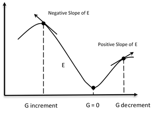
As you can see, we move in the direction in which the gradient G of the function E is minimal.
Stochastic gradient descent
In GD optimization, we compute the cost gradient based on the complete training set; hence, we sometimes also call it batch GD. In the case of very large datasets, using GD can be quite costly, since we are only taking a single step for one pass over the training set. Thus, the larger the training set, the slower our algorithm updates the weights and the longer it may take until it converges to the global cost minimum.
An alternative approach and the fastest of gradient descent, and for this reason, used in DNNs, is the Stochastic Gradient Descent (SGD).
In SGD, we use only one training sample from the training set to do the update for a parameter in a particular iteration. Here, the term stochastic comes from the fact that the gradient based on a single training sample is a stochastic approximation of the true cost gradient.
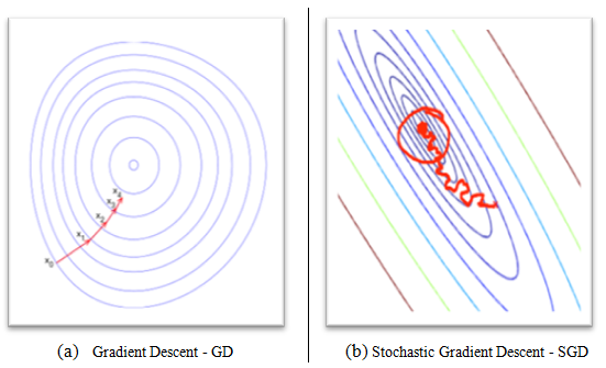
Due to its stochastic nature, the path toward the global cost minimum is not direct, as in GD, but may zigzag if we are visualizing the cost surface in a 2D space (see the following figure, (b) Stochastic Gradient Descent - SDG).
We can make a comparison between these optimization procedures, showing the next figure, the gradient descent (see the following figure, (a) Gradient Descent - GD) assures that each update in the weights is done in the right direction--the one that minimizes the cost function. With the growth of datasets' size, and more complex computations in each step, SGD came to be preferred in these cases. Here, updates to the weights are done as each sample is processed and, as such, subsequent calculations already use improved weights. Nonetheless, this very reason leads to it incurring some misdirection in minimizing the error function:
Neural network architectures
The way to connect the nodes, the number of layers present, that is, the levels of nodes between input and output, and the number of neurons per layer, defines the architecture of a neural network. There are various types of architecture in neural networks, but this book will focus mainly on two large architectural families.
Multilayer perceptron
In multilayer networks, one can identify the artificial neurons of layers such that:
- Each neuron is connected with all those of the next layer
- There are no connections between neurons belonging to the same layer
- There are no connections between neurons belonging to non-adjacent layers
- The number of layers and of neurons per layer depends on the problem to be solved
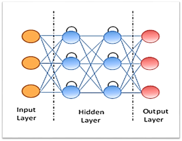
The input and output layers define inputs and outputs; there are hidden layers, whose complexity realizes different behaviors of the network. Finally, the connections between neurons are represented by as many matrices are the pairs of adjacent layers. Each array contains the weights of the connections between the pairs of nodes of two adjacent layers. The feed-forward networks are networks with no loops within the layers.
Following is the graphical representation of multilayer perceptron architecture:

DNNs architectures
Deep Neural Networks (DNNs) are artificial neural networks strongly oriented to deep learning. Where normal procedures of analysis are inapplicable due to the complexity of the data to be processed, such networks are an excellent modeling tool. DNNs are neural networks, very similar to those we have discussed, but they must implement a more complex model (a great number of neurons, hidden layers, and connections), although they follow the learning principles that apply to all machine learning problems (that is, supervised learning).
As they are built, the DNNs work in parallel, so they are able to treat a lot of data. They are a sophisticated statistical system, equipped with a good immunity to errors.
Unlike algorithmic systems where you can examine the output generation step by step, in neural networks, you can also have very reliable results, but sometimes without the ability to understand the reasons for those results. There are no theorems to generate optimal neural networks--the likelihood of getting a good network is all in the hands of its creator, who must be familiar with statistical concepts, and particular attention must be given to the choice of predictor variables.
For brief cheat sheet on the different neural network architecture and their related publications, refer to the website of Asimov Institute at http://www.asimovinstitute.org/neural-network-zoo/.
Finally, we observe that, in order to be productive, the DNNs require training that properly tunes the weights. Training can take a long time if the data to be examined and the variables involved are high, as is often the case when you want optimal results. This section introduces the deep learning architectures that we will cover during the course of this book.
Convolutional Neural Networks
Convolutional Neural Networks (CNNs) has been designed specifically for image recognition. Each image used in learning is divided into compact topological portions, each of which will be processed by filters to search for particular patterns. Formally, each image is represented as a three-dimensional matrix of pixels (width, height, and color), and every sub-portion is put on convolution with the filter set. In other words, scrolling each filter along the image computes the inner product of the same filter and input. This procedure produces a set of feature maps (activation maps) for the various filters. By superimposing the various feature maps of the same portion of the image, we get an output volume. This type of layer is called a convolutional layer.
The following figure shows a typical CNN architecture:

Restricted Boltzmann Machines
A Restricted Boltzmann Machine (RBM) consists of a visible and a hidden layer of nodes, but without visible-visible connections and hidden-hidden by the term restricted. These restrictions allow more efficient network training (training that can be supervised or unsupervised).
This type of neural network can represent with few size of the network a large number of features of the inputs; in fact, the n hidden nodes can represent up to 2n features. The network can be trained to respond to a single question (yes/no), up until (again, in binary terms) a total of 2n questions.
The architecture of the RBM is as follows, with neurons arranged according to a symmetrical bipartite graph:

Autoencoders
Stacked autoencoders are DNNs that are typically used for data compression. Their particular hourglass structure clearly shows the first part of the process, where the input data is compressed, up to the so-called bottleneck, from which the decompression starts.
The output is then an approximation of the input. These networks are not supervised in the pretraining (compression) phase, and the fine-tuning (decompression) phase is supervised:

Recurrent Neural Networks
The fundamental feature of a Recurrent Neural Network (RNN) is that the network contains at least one feedback connection, so the activations can flow around in a loop. It enables the networks to do temporal processing and learn sequences, for example, perform sequence recognition/reproduction or temporal association/prediction. RNN architectures can have many different forms. One common type consists of a standard multilayer perceptron (MLP) plus added loops. These can exploit the powerful non-linear mapping capabilities of the MLP, and also have some form of memory. Others have more uniform structures, potentially with every neuron connected to all the others, and may also have stochastic activation functions. For simple architectures and deterministic activation functions, learning can be achieved using similar gradient descent procedures to those leading to the backpropagation algorithm for feed-forward networks.
The following figure shows a few of the most important types and features of RNNs:
Deep learning framework comparisons
In this section, we will look at some of the most popular frameworks regarding deep learning. In short, almost all libraries provide the possibility of using the graphics processor to speed up the learning process, and are released under an open license and are the result of implementation by university research groups.Before starting the comparison, refer figure 13 which is one of the most complete charts of neural networks till date. If you see the URL and related papers, you will find that the idea of neural networks is pretty old and the software frameworks that we are going to compare below also adapts similar architecture during their framework development:
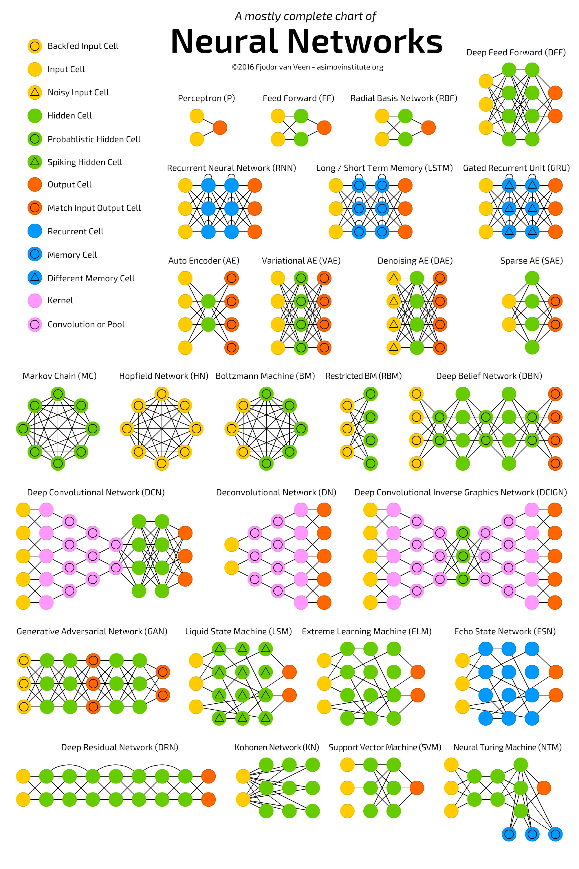
Figure 13: complete charts of neural networks (Source: http://www.asimovinstitute.org/neural-network-zoo/)
- Theano: This is probably the most widespread library. Written in Python, one of the languages most used in the field of machine learning (also in TensorFlow), allows the calculation also GPU, coming to have 24x the performance of the CPU. It allows you to define, optimize, and evaluate complex mathematical expressions such as multidimensional arrays.
- Caffe: This was developed primarily by Berkeley Vision and Learning Center (BVLC), and is a framework designed to stand out in terms of expression, speed, and modularity. Its unique architecture encourages application and innovation by allowing easier transition from calculation of CPU to GPU. The large community of users allowed for considerable development in recent times. It is written in Python, but the installation process can be long due to the numerous support libraries to compile.
- Torch: This is a vast ecosystem for machine learning which offers a large number of algorithms and functions, including those for deep learning and processing of various types of multimedia, such as audio and video data, with particular attention to parallel computing. It provides an excellent interface for the C language and has a large community of users. Torch is a library that extends the scripting language Lua, and is intended to provide a flexible environment for designing and training machine learning systems. Torch is a self-contained and highly portable framework on each platform (for example, Windows, Mac, Linux, and Android) and scripts manage to run on these platforms without modification. The Torch package provides many useful features for different applications.
Finally, the following table provides a summary of each framework's salient features, including TensorFlow, which will be described (of course!!) in the coming chapters:
| TensorFlow | Torch | Caffe | Theano | |
|
Programming language used |
Python and C++ | Lua | C++ | Python |
| GPU card support | Yes | Yes | Yes | By default, no |
| Pros |
|
|
|
|
| Cons |
|
|
|
|
Summary
In this chapter, we introduced some of the fundamental themes of deep learning. It consists of a set of methods that allow a machine learning system to obtain a hierarchical representation of data, on multiple levels. This is achieved by combining simple units, each of which transforms the representation at its own level, starting from the input level, in a representation at a higher level, slightly more abstract.
In recent years, these techniques have provided results never seen before in many applications, such as image recognition and speech recognition. One of the main reasons for the spread of these techniques has been the development of GPU architectures, which considerably reduced the training time of DNNs. There are different DNN architectures, each of which has been developed for a specific problem. We'll talk more about those architectures in later chapters, showing examples of applications created with the TensorFlow framework.
The chapter ended with a brief overview of the implemented deep learning frameworks.
In the next chapter, we begin our journey into deep learning, introducing the TensorFlow software library. We will describe its main features and look at how to install it and set up a first working session.


