


 Download code from GitHub
"By far the greatest danger of Artificial Intelligence is that people conclude too early that they understand it." | ||
| --Eliezer Yudkowsky | ||
Ever thought, why it is often difficult to beat the computer in chess, even for the best players of the game? How Facebook is able to recognize your face amid hundreds of millions of photos? How can your mobile phone recognize your voice, and redirect the call to the correct person, from hundreds of contacts listed?
The primary goal of this book is to deal with many of those queries, and to provide detailed solutions to the readers. This book can be used for a wide range of reasons by a variety of readers, however, we wrote the book with two main target audiences in mind. One of the primary target audiences is undergraduate or graduate university students learning about deep learning and Artificial Intelligence; the second group of readers are the software engineers who already have a knowledge of big data, deep learning, and statistical modeling, but want to rapidly gain knowledge of how deep learning can be used for big data and vice versa.
This chapter will mainly try to set a foundation for the readers by providing the basic concepts, terminologies, characteristics, and the major challenges of deep learning. The chapter will also put forward the classification of different deep network algorithms, which have been widely used by researchers over the last decade. The following are the main topics that this chapter will cover:
Getting started with deep learning
Deep learning terminologies
Deep learning: A revolution in Artificial Intelligence
Classification of deep learning networks
Ever since the dawn of civilization, people have always dreamt of building artificial machines or robots which can behave and work exactly like human beings. From the Greek mythological characters to the ancient Hindu epics, there are numerous such examples, which clearly suggest people's interest and inclination towards creating and having an artificial life.
During the initial computer generations, people had always wondered if the computer could ever become as intelligent as a human being! Going forward, even in medical science, the need of automated machines has become indispensable and almost unavoidable. With this need and constant research in the same field, Artificial Intelligence (AI) has turned out to be a flourishing technology with various applications in several domains, such as image processing, video processing, and many other diagnosis tools in medical science too.
Although there are many problems that are resolved by AI systems on a daily basis, nobody knows the specific rules for how an AI system is programmed! A few of the intuitive problems are as follows:
Google search, which does a really good job of understanding what you type or speak
As mentioned earlier, Facebook is also somewhat good at recognizing your face, and hence, understanding your interests
Moreover, with the integration of various other fields, for example, probability, linear algebra, statistics, machine learning, deep learning, and so on, AI has already gained a huge amount of popularity in the research field over the course of time.
One of the key reasons for the early success of AI could be that it basically dealt with fundamental problems for which the computer did not require a vast amount of knowledge. For example, in 1997, IBM's Deep Blue chess-playing system was able to defeat the world champion Garry Kasparov [1]. Although this kind of achievement at that time can be considered significant, it was definitely not a burdensome task to train the computer with only the limited number of rules involved in chess! Training a system with a fixed and limited number of rules is termed as hard-coded knowledge of the computer. Many Artificial Intelligence projects have undergone this hard-coded knowledge about the various aspects of the world in many traditional languages. As time progresses, this hard-coded knowledge does not seem to work with systems dealing with huge amounts of data. Moreover, the number of rules that the data was following also kept changing in a frequent manner. Therefore, most of the projects following that system failed to stand up to the height of expectation.
The setbacks faced by this hard-coded knowledge implied that those artificial intelligence systems needed some way of generalizing patterns and rules from the supplied raw data, without the need for external spoon-feeding. The proficiency of a system to do so is termed as machine learning. There are various successful machine learning implementations which we use in our daily life. A few of the most common and important implementations are as follows:
Spam detection: Given an e-mail in your inbox, the model can detect whether to put that e-mail in spam or in the inbox folder. A common naive Bayes model can distinguish between such e-mails.
Credit card fraud detection: A model that can detect whether a number of transactions performed at a specific time interval are carried out by the original customer or not.
One of the most popular machine learning models, given by Mor-Yosef et al in 1990, used logistic regression, which could recommend whether caesarean delivery was needed for the patient or not!
There are many such models which have been implemented with the help of machine learning techniques.

Figure 1.1: The figure shows the example of different types of representation. Let's say we want to train the machine to detect some empty spaces in between the jelly beans. In the image on the right side, we have sparse jelly beans, and it would be easier for the AI system to determine the empty parts. However, in the image on the left side, we have extremely compact jelly beans, and hence, it will be an extremely difficult task for the machine to find the empty spaces. Images sourced from USC-SIPI image database
A large portion of performance of the machine learning systems depends on the data fed to the system. This is called representation of the data. All the information related to the representation is called the feature of the data. For example, if logistic regression is used to detect a brain tumor in a patient, the AI system will not try to diagnose the patient directly! Rather, the concerned doctor will provide the necessary input to the systems according to the common symptoms of that patient. The AI system will then match those inputs with the already received past inputs which were used to train the system.
Based on the predictive analysis of the system, it will provide its decision regarding the disease. Although logistic regression can learn and decide based on the features given, it cannot influence or modify the way features are defined. Logistic regression is a type of regression model where the dependent variable has a limited number of possible values based on the independent variable, unlike linear regression. So, for example, if that model was provided with a caesarean patient's report instead of the brain tumor patient's report, it would surely fail to predict the correct outcome, as the given features would never match with the trained data.
These dependencies of the machine learning systems on the representation of the data are not really unknown to us! In fact, most of our computer theory performs better based on how the data are represented. For example, the quality of a database is considered based on how the schema is designed. The execution of any database query, even on a thousand or a million lines of data, becomes extremely fast if the table is indexed properly. Therefore, the dependency of the data representation of the AI systems should not surprise us.
There are many such examples in daily life too, where the representation of the data decides our efficiency. To locate a person amidst 20 people is obviously easier than to locate the same person in a crowd of 500 people. A visual representation of two different types of data representation is shown in the preceding Figure 1.1.
Therefore, if the AI systems are fed with the appropriate featured data, even the hardest problems could be resolved. However, collecting and feeding the desired data in the correct way to the system has been a serious impediment for the computer programmer.
There can be numerous real-time scenarios where extracting the features could be a cumbersome task. Therefore, the way the data are represented decides the prime factors in the intelligence of the system.
Note
Finding cats amidst a group of humans and cats can be extremely complicated if the features are not appropriate. We know that cats have tails; therefore, we might like to detect the presence of tails as a prominent feature. However, given the different tail shapes and sizes, it is often difficult to describe exactly how a tail will look like in terms of pixel values! Moreover, tails could sometimes be confused with the hands of humans. Also, overlapping of some objects could omit the presence of a cat's tail, making the image even more complicated.
From all the above discussions, it can be concluded that the success of AI systems depends mainly on how the data are represented. Also, various representations can ensnare and cache the different explanatory factors of all the disparities behind the data.
Representation learning is one of the most popular and widely practiced learning approaches used to cope with these specific problems. Learning the representations of the next layer from the existing representation of data can be defined as representation learning. Ideally, all representation learning algorithms have this advantage of learning representations, which capture the underlying factors, a subset that might be applicable for each particular sub-task. A simple illustration is given in the following Figure 1.2:
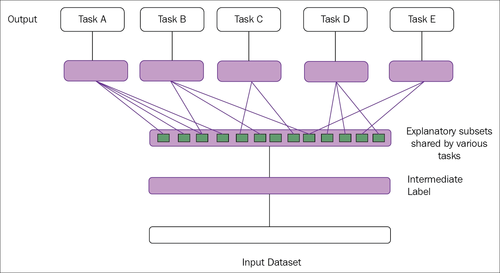
Figure 1.2: The figure illustrates representation learning. The middle layers are able to discover the explanatory factors (hidden layers, in blue rectangular boxes). Some of the factors explain each task's target, whereas some explain the inputs
However, dealing with extracting some high-level data and features from a massive amount of raw data, which requires some sort of human-level understanding, has shown its limitations. There can be many such examples:
Differentiating the cry of two similar age babies.
Identifying the image of a cat's eye at both day and night time. This becomes clumsy, because a cat's eyes glow at night unlike during the daytime.
In all these preceding edge cases, representation learning does not appear to behave exceptionally, and shows deterrent behavior.
Deep learning, a sub-field of machine learning, can rectify this major problem of representation learning by building multiple levels of representations or learning a hierarchy of features from a series of other simple representations and features [2] [8].
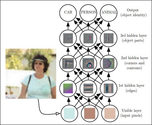
Figure 1.3: The figure shows how a deep learning system can represent the human image by identifying various combinations such as corners and contours, which can be defined in terms of edges. Image reprinted with permission from Ian Goodfellow, Yoshua Bengio, and Aaron Courville, Deep Learning, published by The MIT Press
The preceding Figure 1.3 shows an illustration of a deep learning model. It is generally a cumbersome task for the computer to decode the meaning of raw unstructured input data, as represented by this image, as a collection of different pixel values. A mapping function, which will convert the group of pixels to identify the image, is ideally difficult to achieve. Also, to directly train the computer for these kinds of mapping is almost insuperable. For these types of tasks, deep learning resolves the difficulty by creating a series of subsets of mappings to reach the desired output. Each subset of mappings corresponds to a different set of layer of the model. The input contains the variables that one can observe, and hence , are represented in the visible layers. From the given input we can incrementally extract the abstract features of the data. As these values are not available or visible in the given data, these layers are termed as hidden layers.
In the image, from the first layer of data, the edges can easily be identified just by a comparative study of the neighboring pixels. The second hidden layer can distinguish the corners and contours from the first hidden layer's description of the edges. From this second hidden layer, which describes the corners and contours, the third hidden layer can identify the different parts of the specific objects. Ultimately, the different objects present in the image can be distinctly detected from the third layer.
Deep learning started its journey exclusively in 2006, Hinton et al. in 2006[2]; also Bengio et al. in 2007[3] initially focused on the MNIST digit classification problem. In the last few years, deep learning has seen major transitions from digits to object recognition in natural images. Apart from this, one of the major breakthroughs was achieved by Krizhevsky et al. in 2012 [4] using the ImageNet dataset.
The scope of this book is mainly limited to deep learning, so before diving into it directly, the necessary definitions of deep learning should be discussed.
Many researchers have defined deep learning in many ways, and hence, in the last 10 years, it has gone through many definitions too! The following are few of the widely accepted definitions:
As noted by GitHub, deep learning is a new area of machine learning research, which has been introduced with the objective of moving machine learning closer to one of its original goals: Artificial Intelligence. Deep learning is about learning multiple levels of representation and abstraction, which help to make sense of data such as images, sounds, and texts.
As recently updated by Wikipedia, deep learning is a branch of machine learning based on a set of algorithms that attempt to model high-level abstractions in the data by using a deep graph with multiple processing layers, composed of multiple linear and non-linear transformations.
As the definitions suggest, deep learning can also be considered as a special type of machine learning. Deep learning has achieved immense popularity in the field of data science with its ability to learn complex representation from various simple features. To have an in-depth grip on deep learning, we have listed out a few terminologies which will be frequently used in the upcoming chapters. The next topic of this chapter will help you to lay a foundation for deep learning by providing various terminologies and important networks used for deep learning.
To understand the journey of deep learning in this book, one must know all the terminologies and basic concepts of machine learning. However, if you already have enough insight into machine learning and related terms, you should feel free to ignore this section and jump to the next topic of this chapter. Readers who are enthusiastic about data science, and want to learn machine learning thoroughly, can follow Machine Learning by Tom M. Mitchell (1997) [5] and Machine Learning: a Probabilistic Perspective (2012) [6].
Note
Neural networks do not perform miracles. But, used sensibly, they can produce some amazing results.
Neural networks can be recurrent as well as feed-forward. Feed-forward networks do not have any loop associated in their graph, and are arranged in a set of layers. A network with many layers is said to be a deep network. In simple words, any neural network with two or more layers (hidden) is defined as a deep feed-forward network or feed-forward neural network. Figure 1.4 shows a generic representation of a deep feed-forward neural network.
Deep feed-forward networks work on the principle that with an increase in depth, the network can also execute more sequential instructions. Instructions in sequence can offer great power, as these instructions can point to the earlier instruction.
The aim of a feed-forward network is to generalize some function f. For example, classifier y=f(x) maps from input x to category y. A deep feed-forward network modified the mapping, y=f(x; α), and learns the value of the parameter α, which gives the most appropriate value of the function. The following Figure 1.4 shows a simple representation of the deep-forward network, to provide the architectural difference with the traditional neural network.
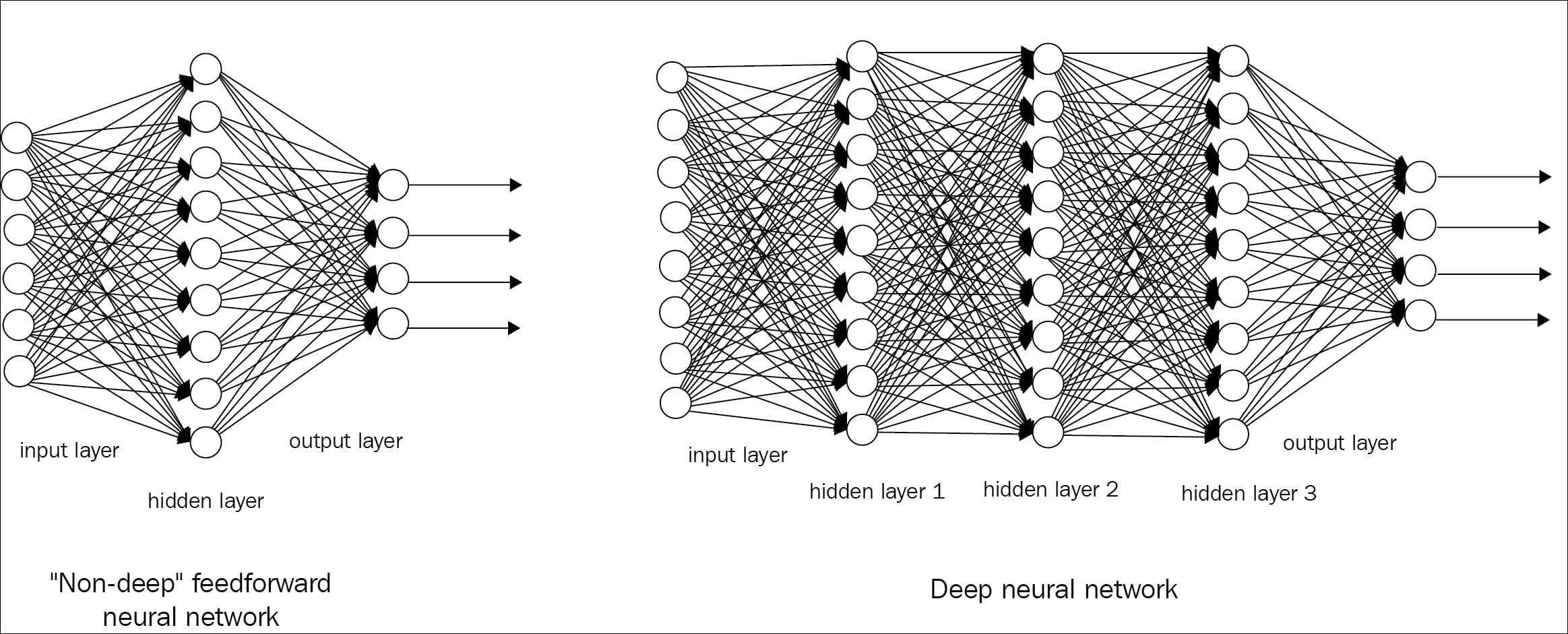
Figure 1.4: Figure shows the representation of a shallow and deep feed-forward network
Datasets are considered to be the building blocks of a learning process. A dataset can be defined as a collection of interrelated sets of data, which is comprised of separate entities, but which can be used as a single entity depending on the use-case. The individual data elements of a dataset are called data points.
The following Figure 1.5 gives the visual representation of the various data points collected from a social network analysis:
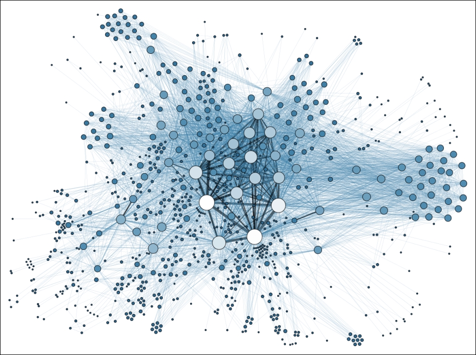
Figure 1.5: Image shows the scattered data points of social network analysis. Image sourced from Wikipedia
Unlabeled data: This part of data consists of the human-generated objects, which can be easily obtained from the surroundings. Some of the examples are X-rays, log file data, news articles, speech, videos, tweets, and so on.
Labelled data: Labelled data are normalized data from a set of unlabeled data. These types of data are usually well formatted, classified, tagged, and easily understandable by human beings for further processing.
From the top-level understanding, machine learning techniques can be classified as supervised and unsupervised learning, based on how their learning process is carried out.
In unsupervised learning algorithms, there is no desired output from the given input datasets. The system learns meaningful properties and features from its experience during the analysis of the dataset. In deep learning, the system generally tries to learn from the whole probability distribution of the data points. There are various types of unsupervised learning algorithms, which perform clustering. To explain in simple words, clustering means separating the data points among clusters of similar types of data. However, with this type of learning, there is no feedback based on the final output, that is, there won't be any teacher to correct you! Figure 1.6 shows a basic overview of unsupervised clustering:
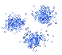
Figure 1.6: Figures shows a simple representation of unsupervised clustering
A real life example of an unsupervised clustering algorithm is Google News. When we open a topic under Google News, it shows us a number of hyper-links redirecting to several pages. Each of these topics can be considered as a cluster of hyper-links that point to independent links.
In supervised learning, unlike unsupervised learning, there is an expected output associated with every step of the experience. The system is given a dataset, and it already knows how the desired output will look, along with the correct relationship between the input and output of every associated layer. This type of learning is often used for classification problems.
The following visual representation is given in Figure 1.7:
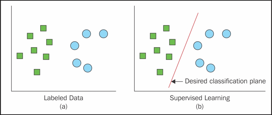
Figure 1.7: Figure shows the classification of data based on supervised learning
Real-life examples of supervised learning include face detection, face recognition, and so on.
Although supervised and unsupervised learning look like different identities, they are often connected to each other by various means. Hence, the fine line between these two learnings is often hazy to the student fraternity.
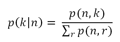
The preceding statement can be formulated with the following mathematical expression:
The general product rule of probability states that for an n number of datasets n ε ℝt,the joint distribution can be fragmented as follows:
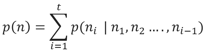
The distribution signifies that the appeared unsupervised problem can be resolved by t number of supervised problems. Apart from this, the conditional probability of p (k | n), which is a supervised problem, can be solved using unsupervised learning algorithms to experience the joint distribution of p (n, k).
Although these two types are not completely separate identities, they often help to classify the machine learning and deep learning algorithms based on the operations performed. In generic terms, cluster formation, identifying the density of a population based on similarity, and so on are termed as unsupervised learning, whereas structured formatted output, regression, classification, and so on are recognized as supervised learning.
As the name suggests, in this type of learning both labelled and unlabeled data are used during the training. It's a class of supervised learning which uses a vast amount of unlabeled data during training.
For example, semi-supervised learning is used in a Deep belief network (explained later), a type of deep network where some layers learn the structure of the data (unsupervised), whereas one layer learns how to classify the data (supervised learning).
In semi-supervised learning, unlabeled data from p (n) and labelled data from p (n, k) are used to predict the probability of k, given the probability of n, or p (k | n).
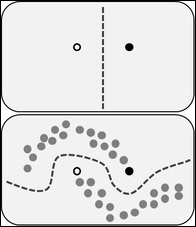
Figure 1.8: Figure shows the impact of a large amount of unlabelled data during the semi-supervised learning technique. Figure obtained from Wikipedia
In the preceding Figure 1.8, at the top it shows the decision boundary that the model uses after distinguishing the white and black circles. The figure at the bottom displays another decision boundary, which the model embraces. In that dataset, in addition to two different categories of circles, a collection of unlabeled data (grey circle) is also annexed. This type of training can be viewed as creating the cluster, and then marking those with the labelled data, which moves the decision boundary away from the high-density data region.
The preceding Figure 1.8 depicts the illustration of semi-supervised learning. You can refer to Chapelle et al.'s book [7] to know more about semi-supervised learning methods.
So, as you have already got a foundation in what Artificial Intelligence, machine learning, and representation learning are, we can now move our entire focus to elaborate on deep learning with further description.
From the previously mentioned definitions of deep learning, two major characteristics of deep learning can be pointed out, as follows:
A way of experiencing unsupervised and supervised learning of the feature representation through successive knowledge from subsequent abstract layers
A model comprising of multiple abstract stages of non-linear information processing
Deep Neural Network (DNN): This can be defined as a multilayer perceptron with many hidden layers. All the weights of the layers are fully connected to each other, and receive connections from the previous layer. The weights are initialized with either supervised or unsupervised learning.
Recurrent Neural Networks (RNN): RNN is a kind of deep learning network that is specially used in learning from time series or sequential data, such as speech, video, and so on. The primary concept of RNN is that the observations from the previous state need to be retained for the next state. The recent hot topic in deep learning with RNN is Long short-term memory (LSTM).
Deep belief network (DBN): This type of network [9] [10] [11] can be defined as a probabilistic generative model with visible and multiple layers of latent variables (hidden). Each hidden layer possesses a statistical relationship between units in the lower layer through learning. The more the networks tend to move to higher layers, the more complex relationship becomes. This type of network can be productively trained using greedy layer-wise training, where all the hidden layers are trained one at a time in a bottom-up fashion.
Boltzmann machine (BM): This can be defined as a network that is a symmetrically connected, neuron-like unit, which is capable of taking stochastic decisions about whether to remain on or off. BMs generally have a simple learning algorithm, which allows them to uncover many interesting features that represent complex regularities in the training dataset.
Restricted Boltzmann machine (RBM): RBM, which is a generative stochastic Artificial Neural Network, is a special type of Boltzmann Machine. These types of networks have the capability to learn a probability distribution over a collection of datasets. An RBM consists of a layer of visible and hidden units, but with no visible-visible or hidden-hidden connections.
Convolutional neural networks: Convolutional neural networks are part of neural networks; the layers are sparsely connected to each other and to the input layer. Each neuron of the subsequent layer is responsible for only a part of the input. Deep convolutional neural networks have accomplished some unmatched performance in the field of location recognition, image classification, face recognition, and so on.
Deep auto-encoder: A deep auto-encoder is a type of auto-encoder that has multiple hidden layers. This type of network can be pre-trained as a stack of single-layered auto-encoders. The training process is usually difficult: first, we need to train the first hidden layer to restructure the input data, which is then used to train the next hidden layer to restructure the states of the previous hidden layer, and so on.
Gradient descent (GD): This is an optimization algorithm used widely in machine learning to determine the coefficient of a function (f), which reduces the overall cost function. Gradient descent is mostly used when it is not possible to calculate the desired parameter analytically (for example, linear algebra), and must be found by some optimization algorithm.
In gradient descent, weights of the model are incrementally updated with every single iteration of the training dataset (epoch).
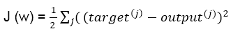
The cost function, J (w), with the sum of the squared errors can be written as follows:
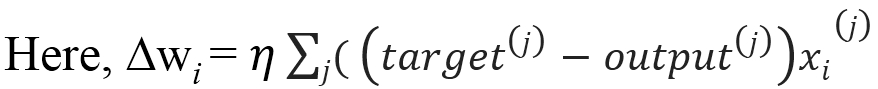
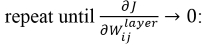
The direction of magnitude of the weight update is calculated by taking a step in the reverse direction of the cost gradient, as follows:
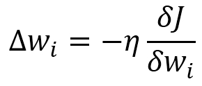
In the preceding equation, η is the learning rate of the network. Weights are updated incrementally after every epoch with the following rule:
                         for one or more epochs,
                           for each weight i,
                             wi:= w + ∆wi
                           end
                         end
Popular examples that can be optimized using gradient descent are Logistic Regression and Linear Regression.
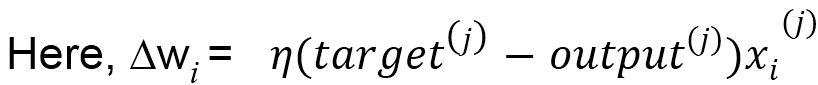
Stochastic Gradient Descent (SGD): Various deep learning algorithms, which operated on a large amount of datasets, are based on an optimization algorithm called stochastic gradient descent. Gradient descent performs well only in the case of small datasets. However, in the case of very large-scale datasets, this approach becomes extremely costly . In gradient descent, it takes only one single step for one pass over the entire training dataset; thus, as the dataset's size tends to increase, the whole algorithm eventually slows down. The weights are updated at a very slow rate; hence, the time it takes to converge to the global cost minimum becomes protracted.
Therefore, to deal with such large-scale datasets, a variation of gradient descent called stochastic gradient descent is used. Unlike gradient descent, the weight is updated after each iteration of the training dataset, rather than at the end of the entire dataset.
                     until cost minimum is reached
                       for each training sample j:
                         for each weight i
                           wi:= w + ∆wi
                         end
                       end
                     end
In the last few years, deep learning has gained tremendous popularity, as it has become a junction for research areas of many widely practiced subjects, such as pattern recognition, neural networks, graphical modelling, machine learning, and signal processing.
The other important reasons for this popularity can be summarized by the following points:
In recent years, the ability of GPU (Graphical Processing Units) has increased drastically
The size of data sizes of the dataset used for training purposes has increased significantly
Recent research in machine learning, data science, and information processing has shown some serious advancements
Detailed descriptions of all these points will be provided in an upcoming topic in this chapter.
An extensive history of deep learning is beyond the scope of this book. However, to get an interest in and cognizance of this subject, some basic context of the background is essential.
In the introduction, we already talked a little about how deep learning occupies a space in the perimeter of Artificial Intelligence. This section will detail more on how machine learning and deep learning are correlated or different from each other. We will also discuss how the trend has varied for these two topics in the last decade or so.
"Deep Learning waves have lapped at the shores of computational linguistics for several years now, but 2015 seems like the year when the full force of the tsunami hit the major Natural Language Processing (NLP) conferences." | ||
| --Dr. Christopher D. Manning, Dec 2015 | ||
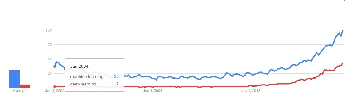
Figure 1.9: Figure depicts that deep learning was in the initial phase approximately 10 years back. However, machine learning was somewhat a trending topic in the researcher's community.
Deep learning is rapidly expanding its territory in the field of Artificial Intelligence, and continuously surprising many researchers with its astonishing empirical results. Machine learning and deep learning both represent two different schools of thought. Machine learning can be treated as the most fundamental approach for AI, where as deep learning can be considered as the new, giant era, with some added functionalities of the subject.
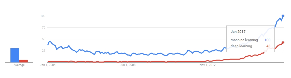
Figure 1.10: Figure depicts how deep learning is gaining in popularity these days, and trying to reach the level of machine learning
However, machine learning has often failed in completely solving many crucial problems of AI, mainly speech recognition, object recognition, and so on.
The performance of traditional algorithms seems to be more challenging while working with high-dimensional data, as the number of random variables keeps on increasing. Moreover, the procedures used to attain the generalization in traditional machine-learning approaches are not sufficient to learn complicated obligations in high-dimensional spaces, which generally impel more computational costs of the overall model. The development of deep learning was mostly motivated by the collapse of the fundamental algorithms of machine learning on such functions, and also to overcome the afore mentioned obstacles.
A large proportion of researchers and data scientists believe that, in the course of time, deep learning will occupy a major portion of Artificial Intelligence, and eventually make machine learning algorithms obsolete. To get a clear idea of this, we looked at the current Google trend of these two fields and came to the following conclusion:
The curve of machine learning has always been the growing stage from the past decade. Deep learning is new, but growing faster than machine learning. When trends are closely observed, one will find that the growth rate is faster for deep learning compared to machine learning.
Both of the preceding Figure 1.9 and Figure 1.10 depict the visualizations of the Google trend.
One of the biggest-known problems that machine learning algorithms face is the curse of dimensionality [12] [13] [14]. This refers to the fact that certain learning algorithms may behave poorly when the number of dimensions in the dataset is high. In the next section, we will discuss how deep learning has given sufficient hope to this problem by introducing new features. There are many other related issues where deep architecture has shown a significant edge over traditional architectures. In this part of the chapter, we would like to introduce the more pronounced challenges as a separate topic.
The curse of dimensionality can be defined as the phenomena which arises during the analysis and organization of data in high-dimensional spaces (in the range of thousands or even higher dimensions). Machine learning problems face extreme difficulties when the number of dimensions in the dataset is high. High dimensional data are difficult to work with because of the following reasons:
With the increasing number of dimensions, the number of features will tend to increase exponentially, which eventually leads to an increase in noise.
In standard practice, we will not get a high enough number of observations to generalize the dataset.
A straightforward explanation for the curse of dimensionality could be combinatorial explosion. As per combinatorial explosion, with the collection of a number of variables, an enormous combination could be built. For example, with n binary variables, the number of possible combinations would be O (2n). So, in high-dimensional spaces, the total number of configurations is going to be almost uncountable, much larger than our number of examples available - most of the configurations will not have such training examples associated with them. Figure 1.11 shows a pictorial representation of a similar phenomenon for better understanding.
Therefore, this situation is cumbersome for any machine learning model, due to the difficulty in the training. Hughes effect [15] states the following:
"With a fixed number of training samples, the predictive power reduces as the dimensionality increases."
Hence, the achievable precision of the model almost collapses as the number of explanatory variables increases.
To cope with this scenario, we need to increase the size of the sample dataset fed to the system to such an extent that it can compete with the scenario. However, as the complexity of data also increases, the number of dimensions almost reaches one thousand. For such cases, even a dataset with hundreds of millions of images will not be sufficient.
Deep learning, with its deeper network configuration, shows some success in partially solving this problem. This contribution is mostly attributed to the following reasons:
Now, the researchers are able to manage the model complexity by redefining the network structure before feeding the sample for training
Deep convolutional networks focus on the higher level features of the data rather than the fundamental level information, which extensively further reduces the dimension of features
Although deep learning networks have given some insights to deal with the curse of dimensionality, they are not yet able to completely conquer the challenge. In Microsoft's recent research on super deep neural networks, they have come up with 150 layers; as a result, the parameter space has grown even bigger. The team has explored the research with even deep networks almost reaching to 1000 layers; however, the result was not up to the mark due to overfitting of the model!
Note
Over-fitting in machine learning: The phenomenon when a model is over-trained to such an extent that it gives a negative impact to its performance is termed as over-fitting of the model. This situation occurs when the model learns the random fluctuations and unwanted noise of the training datasets. The consequences of these phenomena are unsatisfactory--the model is not able to behave well with the new dataset, which negatively impacts the model's ability to generalize.
Under-fitting in machine learning: This refers to a situation when the model is neither able to perform with the current dataset nor with the new dataset. This type of model is not suitable, and shows poor performance with the dataset.
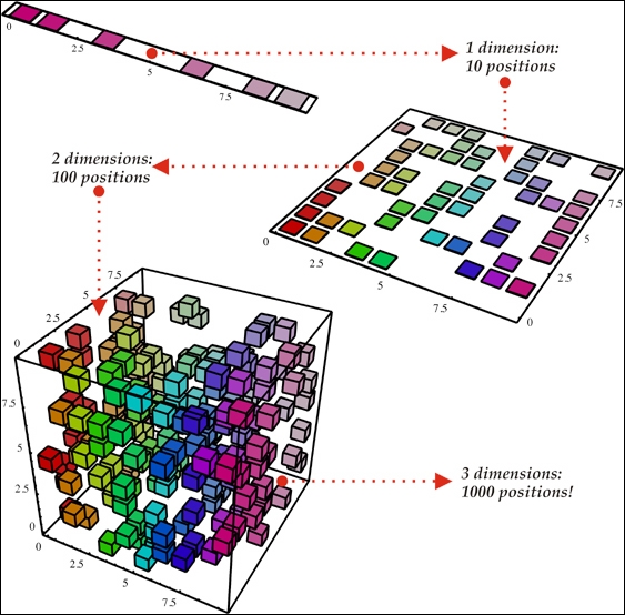
Figure 1.11: Figure shows that with the increase in the number of dimensions from one to three, from top to bottom, the number of random variables might increase exponentially. Image reproduced with permission from Nicolas Chapados from his article DataMining Algorithms for Actuarial Ratemaking.
In the 1D example (top) of the preceding figure, as there are only 10 regions of interest, it should not be a tough task for the learning algorithm to generalize correctly. However, with the higher dimension 3D example (bottom), the model needs to keep track of all the 10*10*10=1000 regions of interest, which is much more cumbersome (or almost going to be an impossible task for the model). This can be used as the simplest example of the curse of dimensionality.
The vanishing gradient problem [16] is the obstacle found while training the Artificial neural networks, which is associated with some gradient-based method, such as Backpropagation. Ideally, this difficulty makes learning and training the previous layers really hard. The situation becomes worse when the number of layers of a deep neural network increases aggressively.
The gradient descent algorithms particularly update the weights by the negative of the gradient multiplied by small scaler value (lies between 0 and 1).
As shown in the preceding equations, we will repeat the gradient until it reaches zero. Ideally, though, we generally set some hyper-parameter for the maximum number of iterations. If the number of iterations is too high, the duration of the training will also be longer. On the other hand, if the number of iterations becomes imperceptible for some deep neural network, we will surely end up with inaccurate results.
In the vanishing gradient problem, the gradients of the network's output, with respect to the parameters of the previous layers, become extremely small. As a result, the resultant weight will not show any significant change with each iteration. Therefore, even a large change in the value of parameters for the earlier layers does not have a significant effect on the overall output. As a result of this problem, the training of the deep neural networks becomes infeasible, and the prediction of the model becomes unsatisfactory. This phenomenon is known as the vanishing gradient problem. This will result in some elongated cost function, as shown in next Figure 1.12:
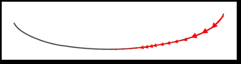
Figure 1.12: Image of a flat gradient and an elongated cost function
An example with large gradient is also shown in the following Figure 1.13, where the gradient descent can converge quickly:
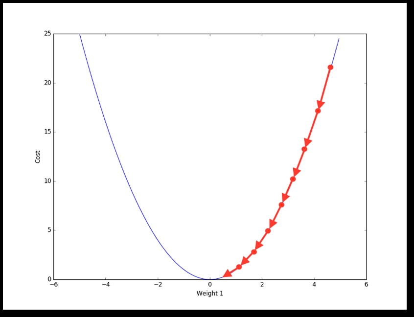
Figure 1.13: Image of a larger gradient cost function; hence the gradient descent can converge much more quickly
This is a substantial challenge in the success of deep learning, but now, thanks to various different techniques, this problem has been overcome to some extent. Long short-term memory (LSTM) network was one of the major breakthroughs which nullified this problem in 1997. A detailed description is given in Chapter 4, Recurrent Neural Network. Also, some researchers have tried to resolve the problem with different techniques, with feature preparation, activation functions, and so on.
All the deep networks are mostly based on the concept of distributed representations, which is the heart of theoretical advantage behind the success of deep learning algorithms. In the context of deep learning, distributed representations are multiscale representations, and are closely related to multiscale modelling of theoretical chemistry and physics. The basic idea behind a distributed representation is that the perceived feature is the result of multiple factors, which work as a combination to produce the desired results. A daily life example could be the human brain, which uses distributed representation for disguising the objects in the surroundings.
An Artificial neural network, in this kind of representation, will be built in such a way that it will have numerous features and layers required to represent our necessary model. The model will describe the data, such as speech, video, or image, with multiple interdependent layers, where each of the layers will be responsible for describing the data at a different level of scale. In this way, the representation will be distributed across many layers, involving many scales. Hence, this kind of representation is termed as distributed representation.
Note
A distributed representation is dense in nature. It follows a many-to-many relationship between two types of representations. One concept can be represented using more than one neuron. On the other hand, one neuron depicts more than one concept.
The traditional clustering algorithms that use non-distributed representation, such as nearest-neighbor algorithms, decision trees, or Gaussian mixtures, all require O(N) parameters to distinguish O(N) input regions. At one point of time, one could hardly have believed that any other algorithm could behave better than this! However, the deep networks, such as sparse coding, RBM, multi-layer neural networks, and so on, can all distinguish as many as O(2k) number of input regions with only O(N) parameters (where k represents the total number of non-zero elements in sparse representation, and k=N for other non-sparse RBMs and dense representations).
In these kinds of operations, either same clustering is applied on different parts of the input, or several clustering takes place in parallel. The generalization of clustering to distributed representations is termed as multi-clustering.
The exponential advantage of using distributed representation is due to the reuse of each parameter in multiple examples, which are not necessarily near to each other. For example, Restricted Boltzmann machine could be an appropriate example in this case. However, with local generalization, non-identical regions in the input space are only concerned with their own private set of parameters.
The key advantages are as follows:
The representation of the internal structure of data is robust in terms of damage resistance and graceful degradation
They help to generalize the concepts and relations among the data, hence enabling the reasoning abilities.
The following Figure 1.14 represents a real-time example of distributed representations:
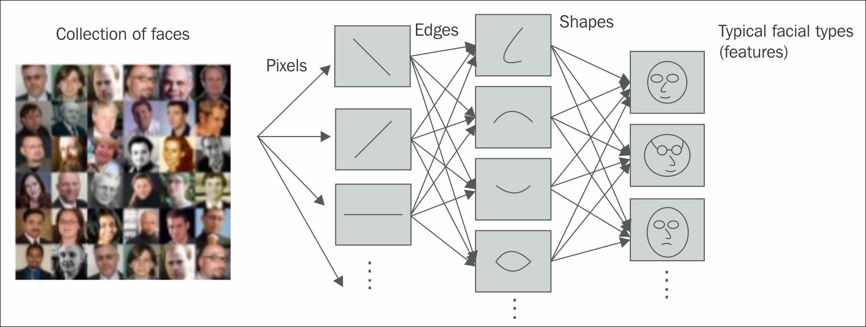
Figure 1.14: Figure shows how distributed representation helped the model to distinguish among various types of expressions in the images
Artificial neural networks in machine learning are often termed as new generation neural networks by many researchers. Most of the learning algorithms that we hear about were essentially built so as to make the system learn exactly the way the biological brain learns. This is how the name Artificial neural networks came about! Historically, the concept of deep learning emanated from Artificial neural networks (ANN). The practice of deep learning started back in the 1960s, or possibly even earlier. With the rise of deep learning, ANN, has gained more popularity in the research field.
Multi-Layer Perceptron (MLP) or feed-forward neural networks with many hidden intermediate layers which are referred to as deep neural networks (DNN), are some good examples of the deep architecture model. The first popular deep architecture model was published by Ivakhnenko and Lapa in 1965 using supervised deep feed-forward multilayer perceptron [17].
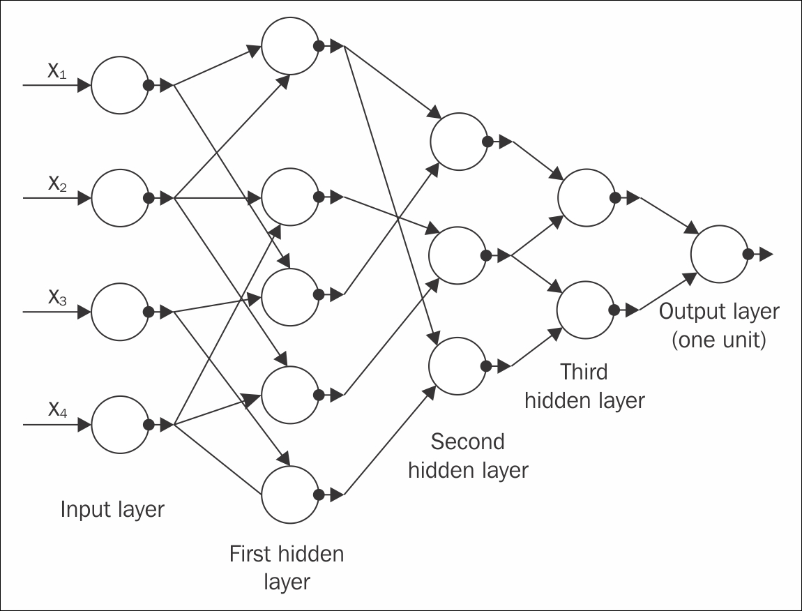
Figure 1.15: The GMDH network has four inputs (the component of the input vector x), and one output y ,which is an estimate of the true function y= f(x) = y
Another paper from Alexey Ivakhnenko, who was working at that time on a better prediction of fish population in rivers, used the group method of data handling algorithm (GMDH), which tried to explain a type of deep network with eight trained layers, in 1971. It is still considered as one of most popular papers of the current millennium[18]. The preceding Figure 1.15 shows the GMDH network of four inputs.
Going forward, Backpropagation (BP), which was a well-known algorithm for learning the parameters of similar type of networks, found its popularity during the 1980s. However, networks having a number of hidden layers are difficult to handle due to many reasons, hence, BP failed to reach the level of expectation [8] [19]. Moreover, backpropagation learning uses the gradient descent algorithm, which is based on local gradient information, and these operations start from some random initial data points. While propagating through the increasing depth of networks, these often get collected in some undesired local optima; hence, the results generally get stuck in poor solutions.
The optimization constraints related to the deep architecture model were pragmatically reduced when an efficient, unsupervised learning algorithm was established in two papers [8] [20]. The two papers introduced a class of deep generative models known as a Deep belief network (DBN).
In 2006, two more unsupervised deep models with non-generative, non-probabilistic features were published, which became immensely popular with the researcher community. One is an energy-based unsupervised model [21], and the other is a variant of auto-encoder with subsequent layer training, much like the previous DBN training [3]. Both of these algorithms can be efficiently used to train a deep neural network, almost exactly like the DBN.
Since 2006, the world has seen a tremendous explosion in the research of deep learning. The subject has seen continuous exponential growth, apart from the traditional shallow machine learning techniques.
Based on the learning techniques mentioned in the previous topics of this chapter, and depending on the use case of the techniques and architectures used, deep learning networks can be broadly classified into two distinct groups.
Many deep learning networks fall under this category, such as Restricted Boltzmann machine, Deep Belief Networks, Deep Boltzmann machine, De-noising Autoencoders, and so on. Most of these networks can be used to engender samples by sampling within the networks. However, a few other networks, for example sparse coding networks and the like, are difficult to sample, and hence, are, not generative in nature.
A popular deep unsupervised model is the Deep Boltzmann machine (DBM) [22] [23] [24] [25]. A traditional DBM contains many layers of hidden variables; however, the variables within the same layer have no connections between them. The traditional Boltzmann machine (BM), despite having a simpler algorithm, is too much complex to study and very slow to train. In a DBM, each layer acquires higher-order complicated correlations between the responses of the latent features of the previous layers. Many real-life problems, such as object and speech recognition, which require learning complex internal representations, are much easier to solve with DBMs.
A DBM with one hidden layer is termed as a Restricted Boltzmann machine (RBM). Similar to a DBM, an RBM does not have any hidden-to-hidden and visible-to-visible connections. The crucial property of an RBM is reflected in constituting many RBMs. With numerous latent layers formed, the feature activation of a previous RBM acts as the input training data for the next. This kind of architecture generates a different kind of network named Deep belief network (DBN). Various applications of the Restricted Boltzmann machine and Deep belief network are discussed in detail in Chapter 5 , Restricted Boltzmann Machines.
A primary component of DBN is a set of layers, which reduces its time complexity linear of size and depth of the networks. Along with DBN property, which could overcome the major drawback of BP by starting the training from some desired initialization data points, it has other attractive catching characteristics too. Some of them are listed as follows:
DBN can be considered as a probabilistic generative model.
With hundreds of millions of parameters, DBNs generally undergo the over-fitting problem. Also, the deep architecture, due to its voluminous dataset, often experiences the under-fitting problem. Both of these problems can be effectively diminished in the pre-training step.
Effective uses of unlabeled data are practiced by DBN.
One more deep generative network, which can be used for unsupervised (as well as supervised) learning is the sum-product network (SPN) [26], [27]. SPNs are deep networks, which can be viewed as directed acyclic graphs, where the leaves of the graph are the observed variables, and the internal nodes are the sum and product operations. The 'sum' nodes represent the mixture models, and the 'product' nodes frame the feature hierarchy. SPNs are trained using the expectation-maximization algorithm together with Back propagation. The major hindrance in learning SPNs is that the gradient rapidly diminishes when moving towards the deep layers. Specifically, the standard gradient descent of the regular deep neural networks generated from the derivative of the conditional likelihood, goes through the tribulation. A solution to reduce this problem is to substitute the marginal inference with the most probable state of the latent variables, and then disseminate the gradient through this. An exceptional outcome on small-scale image recognition was presented by Domingo and Gens in [28]. The following Figure 1.16 shows a sample SPN network for better understanding. It shows a block diagram of the sum-product network:
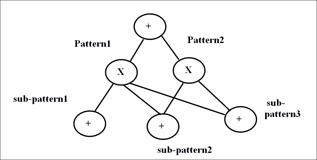
Figure 1.16: Block diagram of sum-product network
Another type of popular deep generative network, which can be used as unsupervised (as well as supervised) learning, is the Recurrent neural network (RNN). The depth of this type of network directly depends on the length of the input data sequence. In the unsupervised RNN model, experiences from previous data samples are used to predict the future data sequence. RNNs have been used as an excellent powerful model for data sequencing text or speech, however, their popularity has recently decreased due to the rise of vanishing gradient problems [29] [16]. Using stochastic curvature estimates, Hessian-free optimization [30] has somewhat overcome the limitations. Recently, Bengio et al. [31] and Sutskever [32] have come out with different variations to train the generating RNNs, which outperform the Hessian-free optimization models. RNN is further elucidated in this book in Chapter 4 , Recurrent Neural Network.
Among the other subclasses of unsupervised deep networks, the energy-based deep models are mostly known architecture [33] [34]. A typical example of the unsupervised model category of deep networks is deep autoencoder. Most of the variants of deep autoencoder are generative in nature; however, the properties and implementations generally vary from each other. Popular examples are predictive sparse coders, Transforming Autoencoder, De-noising Autoencoder and their stacked versions, and so on. Auto-encoders are explained in detail in Chapter 6 , Autoencoders.
Most of the discriminative techniques used in supervised learning are shallow architectures such as Hidden Marcov models [35], [36], [37], [38], [39], [40], [41] or conditional random fields. However, recently, a deep-structured conditional random field model has evolved, by passing the output of every lower layer as the input of the higher layers. There are multiple versions of deep-structured conditional random fields which have been successfully accomplished to for natural language processing, phone recognition, language recognition, and so on. Although discriminative approaches are successful for deep-architectures, they have not been able to reach the expected outcome yet.
As mentioned in the previous section, RNNs have been used for unsupervised learning. However, RNNs can also be used as a discriminative model and trained with supervised learning. In this case, the output becomes a label sequence related to the input data sequence. Speech recognition techniques have already seen such discriminative RNNs a long time ago, but with very little success. Paper [42] shows that a Hidden Marcov Model was used to mutate the RNN classification outcome into a labelled sequence. But unfortunately, the use of Hidden Marcov model for all these reasons did not take enough advantage of the full capability of RNNs.
A few other methods and models have recently been developed for RNNs, where the fundamental idea was to consider the RNN output as some conditional distributions, and distribute all over the possible input sequences [43], [44],[45],[46]. This helped RNNs to undergo sequence classification while embedding the long-short-term-memory to its model. The major benefit was that it neither required the pre-segmentation of the training dataset, nor the post-processing of the outputs. Basically, the segmentation of the dataset is automatically performed by the algorithm, and one differentiable objective function could be derived for optimization of the conditional distributions across the label sequence. The effectiveness of this type of algorithm is extensively applicable for handwriting recognition operations.
One more popular type of discriminative deep architecture is the convolutional neural network (CNN). In CNN, each module comprises of a convolutional layer and one pooling layer. To form a deep model, the modules are generally stacked one on top of the other, or with a deep neural network on the top of it. The convolutional layer helps to share many weights, and the pooling layer segregates the output of the convolutional later, minimizing the rate of data from the previous layer. CNN has been recognized as a highly efficient model, especially for tasks like image recognition, computer vision, and so on. Recently, with specific modifications in CNN design, it has also been found equally effective in speech recognition too. Time-delay neural network (TDNN) [47] [48], originated for early speech recognition, is a special case for convolutional neural network, and can also be considered its predecessor.
In this type of model, the weight sharing is limited to only time dimension, and no pooling layer is present. Chapter 3 , Convolutional Neural Networks discusses the concept and applications of CNNs in depth.
Deep learning, with its many models, has a wide range of applications too. Many of the top technology companies, such as Facebook, Microsoft, Google, Adobe, IBM, and so on are extensively using deep learning. Apart from computer science, deep learning has also provided valuable contributions to other scientific fields as well.
Modern CNNs used for object recognition have given a major insight into visual processing, which even neuroscientists can explore further. Deep learning also provides the necessary functional tools for processing large-scale data, and to make predictions in scientific fields. This field is also very successful in predicting the behaviors of molecules in order to enhance the pharmaceutical researches.
To summarize, deep learning is a sub-field of machine learning, which has seen exceptional growth in usefulness and popularity due to its much wider applicability. However, the coming years should be full of challenges and opportunities to ameliorate deep learning even further, and explore the subject for new data enthusiasts.
Note
To help the readers to get more insights into deep learning, here are a few other excellent and frequently updated reading lists available online: http://deeplearning.net/tutorial/ http://ufldl.stanford.edu/wiki/index.php/UFLDL_Tutorial http://deeplearning.net/reading-list/
Over the past decade, we have had the privilege of hearing about the greatest inventions of deep learning from many of the great scientists and companies working in Artificial Intelligence. Deep learning is an approach to machine learning which has shown tremendous growth in its usefulness and popularity in the last few years. The reason is mostly due to its capability to work with large datasets involving high dimensional data, resolving major issues such as vanishing gradient problems, and so on, and techniques to train deeper networks. In this chapter, we have explained most of these concepts in detail, and have also classified the various algorithms of deep learning, which will be elucidated in detail in subsequent chapters.
The next chapter of this book will introduce the association of big data with deep learning. The chapter will mainly focus on how deep learning plays a major role in extracting valuable information from large-scale data.
