More than 20 years have passed since the Python programming language was released. During that period, it has evolved and increased its user base. Python is currently the most popular programming language in the world.

In this book, we will use this powerful language to implement a deep learning system. This chapter explains Python briefly and describes how to use it. If you are familiar with Python, NumPy, and Matplotlib, you can skip this chapter.

Python is a simple programming language that is easy to read and learn. It is open-source software that you can use as you like for free. You can write a program that uses English-like grammar without the time-consuming compilation. This makes Python easy to use and, therefore a great choice for beginner programmers. In fact, many computer science courses in universities and professional schools choose Python as the first language they teach.

Python enables you to write both readable and high-performance (fast) code. If massive data processing and high-speed responses are required, Python will meet your needs. This is why Python is a favorite both with beginners and professionals. Cutting-edge IT companies such as Google, Microsoft, and Facebook frequently use Python.

Python is often used in scientific fields, particularly in machine learning and data science. Because of its high performance and excellent libraries for numerical calculations and statistical processing (NumPy and SciPy, for example), Python occupies a solid position in the realm of data science. It is often used as the backbone of deep learning frameworks such as Caffe, TensorFlow, and PyTorch, which provide Python interfaces. Therefore, learning Python is also useful when you wish to use a framework for deep learning.

Python is an optimal programming language, particularly in data science, as it offers various user-friendly and efficient features for beginners and professionals alike. For these reasons, it is the natural choice for achieving the goal of this book: Deep Learning from the Basics.

The following section describes some precautions you will need to take when installing Python in your environment (PC).

Python Versions

Python has two major versions: version 2 and version 3. Currently, both are in active use. So, when you install Python, you must carefully choose which version to install. These two versions are not completely compatible (to be accurate, no backward compatibility is available). Some programs written in Python 3 cannot be run in Python 2. This book uses Python 3. If you have only Python 2 installed, installing Python 3 is recommended.

External Libraries That We Use

The goal of this book is to implement Deep Learning from the Basics. So, our policy is that we will use external libraries as little as possible, but we will use the following two libraries by way of exception: NumPy and Matplotlib. We will use these two libraries to implement deep learning efficiently.

NumPy is a library for numerical calculations. It provides many convenient methods for handling advanced mathematical algorithms and arrays (matrices). To implement deep learning in this book, we will use these convenient methods for efficient implementation.

Matplotlib is a library for drawing graphs. You can use Matplotlib to visualize experimental results and visually check the data while executing deep learning. This book uses these libraries to implement deep learning.

This book uses the following programming language and libraries:

• Python 3
• NumPy
• Matplotlib

Now, we will describe how to install Python for those who need to install it. If you have already met these requirements, you can skip this section.

Anaconda Distribution

Although numerous methods are available for installing Python, this book recommends that you use a distribution called Anaconda. Distributions contain the required libraries so that the user can install them collectively. The Anaconda distribution focuses on data analysis. It also contains libraries useful for data analysis, such as NumPy and Matplotlib, as described earlier.

As we mentioned previously, this book uses Python 3. Therefore, you will need to install the Anaconda distribution for Python 3. Use the following link to download the distribution suitable for your OS and install it:

https://docs.anaconda.com/anaconda/install/

After installing Python, start by checking the version. Open a Terminal (Command Prompt for Windows) and enter the python --version command. This command outputs the version of Python you have installed:

$ python --version
Python 3.4.1 :: Anaconda 2.1.0 (x86_64)

If Python 3.4.1 (the number will be different, depending on your installed version) is displayed, as shown in the preceding code, then Python 3 has been installed successfully. Now, enter python and start the Python interpreter:

$ python
Python 3.4.1 |Anaconda 2.1.0 (x86_64)| (default, Sep 10 2014, 17:24:09) [GCC 4.2.1 (Apple Inc. build 5577)] on darwin
Type "help", "copyright", "credits" or "license" for more information.
>>>

The Python interpreter is also referred to as interactive mode, through which you can interact with Python to write programs. An interaction means that, for example, the Python interpreter answers 3 when you ask, "What is 1+2?". Enter the following:

>>> 1 + 2
3

Hence, the Python interpreter enables you to write programs interactively. In this book, we will use an interactive mode to work with simple examples of Python programming.

Mathematical Operations

You can conduct mathematical operations, such as addition and multiplication, as follows:

>>> 1 - 2
-1
>>> 4 * 5
20
>>> 7 / 5
1.4
>>> 3 ** 2
9

Here, * means multiplication, / means division, and ** means exponentiation. (3 ** 2 is the second power of 3.) In Python 2, when you divide two integers, an integer is returned. For example, the result of 7/5 is 1. Meanwhile, in Python 3, when you divide two integers, a floating-point number is returned.

Data Types

Programming has data types. A data type indicates the character of the data, such as an integer, a floating-point number, or a string. Python provides the type() function to check the data's type:

>>> type(10)
<class 'int'>
>>> type(2.718)
<class 'float'>
>>> type("hello")
<class 'str'>

The preceding results indicate that 10 is int (integer type), 2.718 is float (floating-point type), and hello is str (string type). The words type and class are sometimes used in the same way. The resulting output, <class 'int'>, can be interpreted as 10 is an int class (type).

Variables

You can define variables by using alphabetical letters such as x and y. You can also use variables to calculate or assign another value to a variable:

>>> x = 10 # Initialize
>>> print(x) 
10
>>> x = 100 # Assign
>>> print(x)
100
>>> y = 3.14
>>> x * y
314.0
>>> type(x * y)
<class 'float'>

Python is a dynamically typed programming language. Dynamic means that the type of a variable is determined automatically, depending on the situation. In the preceding example, the user does not explicitly specify that the type of x is int (integer). Python determines that the type of x is int because it is initialized to an integer, 10. The preceding example also shows that multiplying an integer by a decimal returns a decimal (automatic type conversion). The # symbol comments out subsequent characters, which are ignored by Python.

Lists

You can use a list (array) to assign multiple numbers to a variable:

>>> a = [1, 2, 3, 4, 5] # Create a list
>>> print(a) # Print the content of the list
[1, 2, 3, 4, 5]
>>> len(a) # Get the length of the list
5
>>> a[0] # Access the first element
1
>>> a[4]
5
>>> a[4] = 99 # Assign a value
>>> print(a)
[1, 2, 3, 4, 99]

To access an element, you can write a[0], for example. The number in this [ ] is called an index, which starts from 0 (the index 0 indicates the first element). A convenient notation called slicing is provided for Python lists. You can use slicing to access both a single element and a sublist of the list:

>>> print(a)
[1, 2, 3, 4, 99]
>>> a[0:2] # Obtain from the zero index to the second index (the second one is not included!) 
[1, 2]
>>> a[1:] # Obtain from the first index to the last
[2, 3, 4, 99]
>>> a[:3] # Obtain from the zero index to the third index (the third one is not included!) 
[1, 2, 3]
>>> a[:-1] # Obtain from the first element to the second-last element
[1, 2, 3, 4]
>>> a[:-2] # Obtain from the first element to the third-last element
[1, 2, 3]

You can slice a list by writing a[0:2]. In this example, a[0:2] obtains the elements from the zeroth index to the one before the second index. So, it will show the elements for the zeroth index and the first index only in this case. An index number of -1 indicates the last element, while -2 indicates the second-last element.

Dictionaries

In a list, values are stored with index numbers (0, 1, 2, ...) that start from 0. A dictionary stores data as key/value pairs. Words associated with their meanings are stored in a dictionary, just as in a language dictionary:

>>> me = {'height':180} # Create a dictionary
>>> me['height'] # Access an element
180
>>> me['weight'] = 70 # Add a new element
>>> print(me)
{'height': 180, 'weight': 70}

Boolean

Python has a bool type. Its value is True or False. The operators for the bool type are and, or, and not (a type determines which operators can be used, such as +, -, *, and / for numbers):

>>> hungry = True # Hungry?
>>> sleepy = False # Sleepy?
>>> type(hungry)
<class 'bool'>
>>> not hungry
False
>>> hungry and sleepy 
False
>>> hungry or sleepy 
True

if Statements

You can use if/else to switch a process, depending on a condition:

>>> hungry = True
>>> if hungry:
...  print("I'm hungry")
...
I'm hungry
>>> hungry = False
>>> if hungry:
...    print("I'm hungry") # Indent with spaces
... else:
...     print("I'm not hungry")
...     print("I'm sleepy")
...
I'm not hungry
I'm sleepy

In Python, spaces have an important meaning. In this if statement example, the next statement after if hungry starts with four spaces. This is an indent that indicates the code that is executed when the condition (if hungry) is met. Although you can use tab characters for an indent, Python recommends using spaces.

In Python, use spaces to represent an indent. Four spaces are usually used for each indent level.

for Statements

Use a for statement for a loop:

>>> for i in [1, 2, 3]:
...    print(i)
...
1
2
3

This example outputs the elements of a list, [1, 2, 3]. When you use a for … in …: statement, you can access each element in a dataset, such as a list, in turn.

Functions

You can define a group of processes as a function:

>>> def hello():
...  print("Hello World!")
...
>>> hello()
Hello World!

A function can take an argument:

>>> def hello(object):
...  print("Hello " + object + "!")
...
>>> hello("cat")
Hello cat!

Use + to combine strings.

To close the Python interpreter, enter Ctrl+D (press the D key while holding down the Ctrl key) for Linux and macOS X. Enter Ctrl+Z and press the Enter key for Windows.

The examples shown so far have used a Python interpreter that provides a mode in which you can interact with Python and which is useful for simple experiments. However, it is a little inconvenient if you want to do large processing because you have to enter a program every time. In such a case, you can save a Python program as a file and execute it (at one time). This next section provides examples of Python script files.

Saving in a File

Open your text editor and create a hungry.py file. The hungry.py file has only one line in it, as shown here:

print("I'm hungry!")

Then, open a Terminal (Command Prompt for Windows) and move to the location where the hungry.py file was created. Execute the python command with the argument of the filename, hungry.py. Here,

it is assumed that hungry.py is located in the ~/deep-learning-from-zero/ch01 directory (in the source code provided by this book, hungry.py is located under the ch01 directory):

$ cd ~/deep-learning-from-zero/ch01 # Move to the directory
$ python hungry.py
I'm hungry! 

Thus, you can use the python hungry.py command to run the Python program.

Classes

So far, you have learned about data types such as int and str (you can use the type() function to check the object type). These data types are called built-in data types since they are built into Python. Here, you will define a new class to create your data type. You can also define your original method (function for a class) and attributes.

In Python, you can use the class keyword to define a class. You must use the following format:

class name:
    def __init__ (self, argument, …): # Constructor
        ...
    def method name 1 (self, argument, …): # Method 1
        ...
    def method name 2 (self, argument, …): # Method 2
        ...

The __init__ method is a special method for initialization. This method for initialization is also referred to as a constructor and is called only once when the instance of a class is created. In Python, you need to write self explicitly as the first argument of a method to represent yourself (your instance). (This practice may seem strange to those who are familiar with other languages.)

Create a class as a simple example as shown below, and save the following program as man.py:

class Man:
    def __init__(self, name):
        self.name = name
        print("Initialized!")
    def hello(self):
        print("Hello " + self.name + "!")
    def goodbye(self):
        print("Good-bye " + self.name + "!")
m = Man("David")
m.hello()
m.goodbye()

Execute man.py from the Terminal:

$ python man.py
Initialized!
Hello David!
Good-bye David!

Here, you defined a new class, Man. In the preceding example, an instance (object), m, was created from the Man class.

The constructor (initialization method) of the Man class takes name as an argument and uses it to initialize the instance variable, self.name. An instance variable is a variable that is stored in each instance. In Python, you can create and access an instance variable by appending an attribute name to self.

When implementing deep learning, arrays and matrices are often calculated. The array class of NumPy (numpy.array) provides many convenient methods that are used to implement deep learning. This section provides a brief description of NumPy, which we will use later.

Importing NumPy

NumPy is an external library. The word external here means that NumPy is not included in standard Python. So, you must load (import) the NumPy library first:

>>> import numpy as np

In Python, an import statement is used to import a library. Here, import numpy as np means that numpy is loaded as np. Thus, you can now reference a method for NumPy as np.

Creating a NumPy Array

You can use the np.array() method to create a NumPy array. np.array() takes a Python list as an argument to create an array for NumPy—that is, numpy.ndarray:

>>> x = np.array([1.0, 2.0, 3.0])
>>> print(x)
[ 1. 2. 3.]
>>> type(x)
<class 'numpy.ndarray'>

Mathematical Operations in NumPy

The following are a few sample mathematical operations involving NumPy arrays:

>>> x = np.array([1.0, 2.0, 3.0])
>>> y = np.array([2.0, 4.0, 6.0])
>>> x + y # Add arrays
array([ 3., 6., 9.])
>>> x - y
array([ -1., -2., -3.])
>>> x * y # element-wise product
array([ 2.,	8., 18.])
>>> x / y
array([ 0.5, 0.5, 0.5])

Take note that the numbers of elements of arrays x and y are the same (both are one-dimensional arrays with three elements). When the numbers of elements of x and y are the same, mathematical operations are conducted for each element. If the numbers of elements are different, an error occurs. So, it is important that they are the same. "For each element" is also called element-wise, and the "product of each element" is called an element-wise product.

In addition to element-wise calculations, mathematical operations of a NumPy array and a single number (scalar value) are also available. In that case, calculations are performed between each element of the NumPy array and the scalar value. This feature is called broadcasting (more details on this will be provided later):

>>> x = np.array([1.0, 2.0, 3.0])
>>> x / 2.0
array([ 0.5, 1. , 1.5])

N-Dimensional NumPy Arrays

In NumPy, you can create multi-dimensional arrays as well as one-dimensional arrays (linear arrays). For example, you can create a two-dimensional array (matrix) as follows:

>>> A = np.array([[1, 2], [3, 4]])
>>> print(A)
[[1 2]
[3 4]]
>>> A.shape
(2, 2)
>>> A.dtype
dtype('int64')

Here, a 2x2 matrix, A, was created. You can use shape to check the shape of the matrix, A, and use dtype to check the type of its elements. Here are the mathematical operations of matrices:

>>> B = np.array([[3, 0],[0, 6]])
>>> A + B
array([[ 4, 2],
[ 3, 10]])
>>> A * B
array([[ 3, 0],
[ 0, 24]])

As in arrays, matrices are calculated element by element if they have the same shape. Mathematical operations between a matrix and a scalar (single number) are also available. This is also conducted by broadcasting:

>>> print(A)
[[1 2]
[3 4]]
>>> A * 10
array([[ 10, 20],
[ 30, 40]])

A NumPy array (np.array) can be an N-dimensional array. You can create arrays of any number of dimensions, such as one-, two-, three-, ... dimensional arrays. In mathematics, a one-dimensional array is called a vector, and a two-dimensional array is called a matrix. Generalizing a vector and a matrix is called a tensor. In this book, we will call a two-dimensional array a matrix, and an array of three or more dimensions a tensor or a multi-dimensional array.

Broadcasting

In NumPy, you can also do mathematical operations between arrays with different shapes. In the preceding example, the 2x2 matrix, A, was multiplied by a scalar value of s. Figure 1.1 shows what is done during this operation: a scalar value of 10 is expanded to 2x2 elements for the operation. This smart feature is called broadcasting:

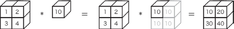
Figure 1.1: Sample broadcasting – a scalar value of 10 is treated as a 2x2 matrix

Here is a calculation for another broadcasting sample:

>>> A = np.array([[1, 2], [3, 4]])
>>> B = np.array([10, 20])
>>> A * B
array([[ 10, 40],
[ 30, 80]])

Here (as shown in Figure 1.2), the one-dimensional array B is transformed so that it has the same shape as the two-dimensional array A, and they are calculated element by element.

Thus, NumPy can use broadcasting to do operations between arrays with different shapes:

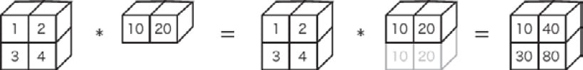
Figure 1.2: Sample broadcasting

Accessing Elements

The index of an element starts from 0 (as usual). You can access each element as follows:

>>> X = np.array([[51, 55], [14, 19], [0, 4]])
>>> print(X)
[[51 55]
[14 19]
[ 0 4]]
>>> X[0]  # 0th row
array([51, 55])
>>> X[0][1] # Element at (0,1)
55

Use a for statement to access each element:

>>> for row in X:
...    print(row)
...
[51 55]
[14 19]
[0 4]

In addition to the index operations described so far, NumPy can also use arrays to access each element:

>>> X = X.flatten( ) # Convert X into a one-dimensional array
>>> print(X)
[51 55 14 19 0 4]
>>> X[np.array([0, 2, 4])] # Obtain the elements of the 0th, 2nd, and 4th indices
array([51, 14, 0])

Use this notation to obtain only the elements that meet certain conditions. For example, the following statement extracts values that are larger than 15 from X:

>>> X > 15
array([ True, True, False, True, False, False], dtype=bool)
>>> X[X>15]
array([51, 55, 19])

An inequality sign used with a NumPy array (X > 15, in the preceding example) returns a Boolean array. Here, the Boolean array is used to extract each element in the array, extracting elements that are True.

Note

It is said that dynamic languages, such as Python, are slower in terms of processing than static languages (compiler languages), such as C and C++. In fact, you should write programs in C/C++ to handle heavy processing. When performance is required in Python, the content of a process is implemented in C/C++. In that case, Python serves as a mediator for calling programs written in C/C++. In NumPy, the main processes are implemented by C and C++. So, you can use convenient Python syntax without reducing performance.

In deep learning experiments, drawing graphs and visualizing data is important. With Matplotlib, you can draw visualize easily by drawing graphs and charts. This section describes how to draw graphs and display images.

Drawing a Simple Graph

You can use Matplotlib's pyplot module to draw graphs. Here is an example of drawing a sine function:

import numpy as np
import matplotlib.pyplot as plt
# Create data
x = np.arange(0, 6, 0.1) # Generate from 0 to 6 in increments of 0.1
y = np.sin(x)
# Draw a graph
plt.plot(x, y)
plt.show()

Here, NumPy's arange method is used to generate the data of [0, 0.1, 0.2, …, 5.8, 5.9] and name it x. NumPy's sine function, np.sin(), is applied to each element of x, and the data rows of x and y are provided to the plt.plot method to draw a graph. Finally, a graph is displayed by plt.show(). When the preceding code is executed, the image shown in Figure 1.3 is displayed:

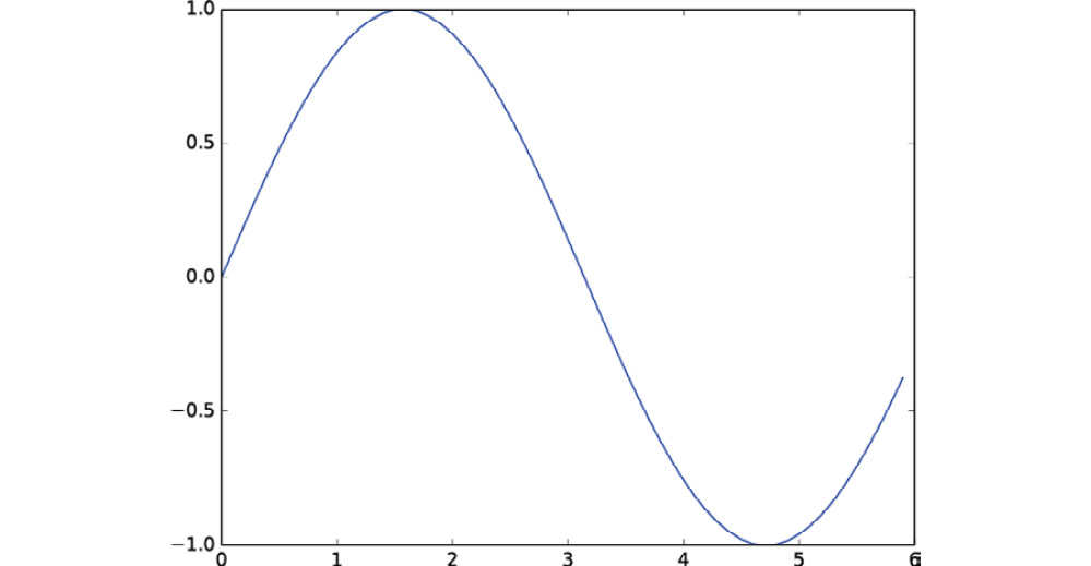
Figure 1.3: Graph of a sine function

Features of pyplot

Here, we will draw a cosine function (cos) in addition to the sine function (sin) we looked at previously. We will use some other features of pyplot to show the title, the label name of the x-axis, and so on:

import numpy as np
import matplotlib.pyplot as plt
# Create data
x = np.arange(0, 6, 0.1) # Generate from 0 to 6 in increments of 0.1
y1 = np.sin(x)
y2 = np.cos(x)
# Draw a graph
plt.plot(x, y1, label="sin")
plt.plot(x, y2, linestyle = "--", label="cos") # Draw with a dashed line
plt.xlabel("x") # Label of the x axis
plt.ylabel("y") # Label of the y axis
plt.title('sin & cos') # Title
plt.legend()
plt.show()

Figure 1.4 shows the resulting graph. You can see that the title of the graph and the label names of the axes are displayed:

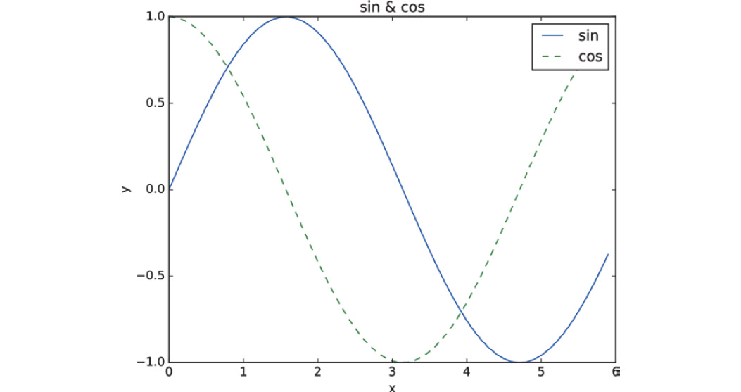
Figure 1.4: Graph of sine and cosine functions

Displaying Images

The imshow() method for displaying images is also provided in pyplot. You can use imread() in the matplotlib.image module to load images, as in the following example:

import matplotlib.pyplot as plt 
from matplotlib.image import imread
img = imread('lena.png') # Load an image (specify an appropriate path!) 
plt.imshow(img)
plt.show()

When you execute this code, the image shown in Figure 1.5 is displayed:

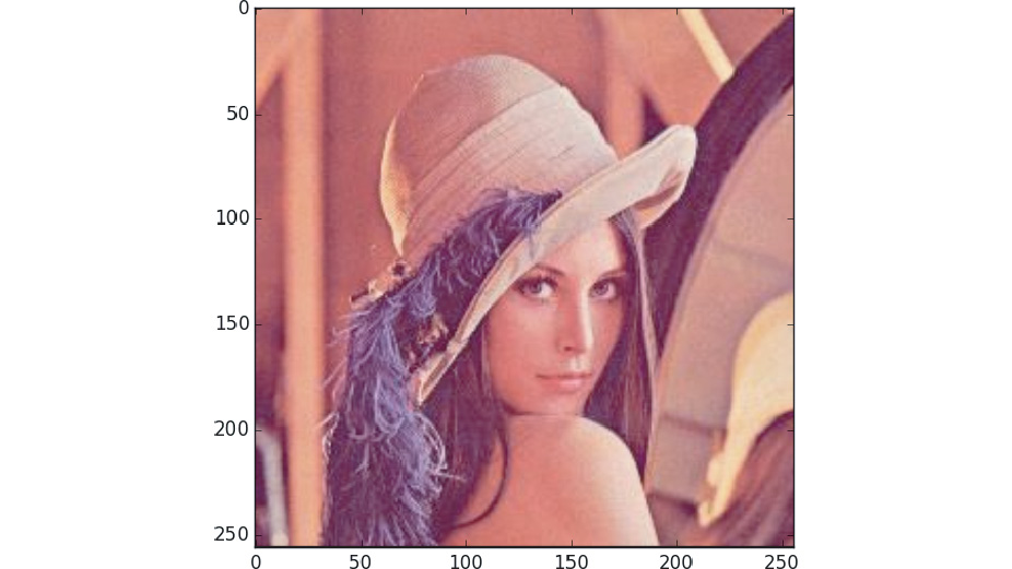
Figure 1.5: Displaying an image

Here, it is assumed that the image, lena.png, is located in the current directory. You need to change the name and path of the file as required, depending on your environment. In the source code provided with this book, lena.png is located under the dataset directory as a sample image. For example, to execute the preceding code from the ch01 directory in the Python interpreter, change the path of the image from lena.png to ../dataset/lena.png for proper operation.

This chapter has given you some of the Python programming basics required to implement deep learning and neural networks. In the next chapter, we will enter the world of deep learning and look at some actual Python code.

This chapter provided only a brief overview of Python. If you want to learn more, the following materials may be helpful. For Python, Bill Lubanovic: Introducing Python, Second Edition, O'Reilly Media, 2019 is recommended. This is a practical primer that elaborately explains Python programming from its basics to its applications. For NumPy, Wes McKinney: Python for Data Analysis, O'Reilly Media, 2012 is easy to understand and well organized. In addition to these books, the Scipy Lecture Notes (https://scipy-lectures.org) website describes NumPy and Matplotlib in scientific and technological calculations in depth. Refer to them if you are interested.

This chapter covered the following points:

• Python is a programming language that is simple and easy to learn.
• Python is an open-source piece of software that you can use as you like.
• This book uses Python 3 to implement deep learning.
• NumPy and Matplotlib are used as external libraries.
• Python provides two execution modes: interpreter and script files.
• In Python, you can implement and import functions and classes as modules.
• NumPy provides many convenient methods for handling multi-dimensional arrays.