


Note
Learning Objectives
By the end of this chapter, you will be able to:
Create pandas DataFrames in Python
Read and write data into different file formats
Slice, aggregate, filter, and apply functions (built-in and custom) to DataFrames
Join DataFrames, handle missing values, and combine different data sources
The way we make decisions in today's world is changing. A very large proportion of our decisions—from choosing which movie to watch, which song to listen to, which item to buy, or which restaurant to visit—all rely upon recommendations and ratings generated by analytics. As decision makers continue to use more of such analytics to make decisions, they themselves become data points for further improvements, and as their own custom needs for decision making continue to be met, they also keep using these analytical models frequently.
The change in consumer behavior has also influenced the way companies develop strategies to target consumers. With the increased digitization of data, greater availability of data sources, and lower storage and processing costs, firms can now crunch large volumes of increasingly granular data with the help of various data science techniques and leverage it to create complex models, perform sophisticated tasks, and derive valuable consumer insights with higher accuracy. It is because of this dramatic increase in data and computing power, and the advancement in techniques to use this data through data science algorithms, that the McKinsey Global Institute calls our age the Age of Analytics.
Several industry leaders are already using data science to make better decisions and to improve their marketing analytics. Google and Amazon have been making targeted recommendations catering to the preferences of their users from their very early years. Predictive data science algorithms tasked with generating leads from marketing campaigns at Dell reportedly converted 50% of the final leads, whereas those generated through traditional methods had a conversion rate of only 17%. Price surges on Uber for non-pass holders during rush hour also reportedly had massive positive effects on the company's profits. In fact, it was recently discovered that price management initiatives based on an evaluation of customer lifetime value tended to increase business margins by 2%–7% over a 12-month period and resulted in a 200%–350% ROI in general.
Although using data science principles in marketing analytics is a proven cost-effective, efficient way for a lot of companies to observe a customer's journey and provide a more customized experience, multiple reports suggest that it is not being used to its full potential. There is a wide gap between the possible and actual usage of these techniques by firms. This book aims to bridge that gap, and covers an array of useful techniques involving everything data science can do in terms of marketing strategies and decision-making in marketing. By the end of the book, you should be able to successfully create and manage an end-to-end marketing analytics pipeline in Python, segment customers based on the data provided, predict their lifetime value, and model their decision-making behavior on your own using data science techniques.
This chapter introduces you to cleaning and preparing data—the first step in any data-centric pipeline. Raw data coming from external sources cannot generally be used directly; it needs to be structured, filtered, combined, analyzed, and observed before it can be used for any further analyses. In this chapter, we will explore how to get the right data in the right attributes, manipulate rows and columns, and apply transformations to data. This is essential because, otherwise, we will be passing incorrect data to the pipeline, thereby making it a classic example of garbage in, garbage out.
When we build an analytics pipeline, the first thing that we need to do is to build a data model. A data model is an overview of the data sources that we will be using, their relationships with other data sources, where exactly the data from a specific source is going to enter the pipeline, and in what form (such as an Excel file, a database, or a JSON from an internet source). The data model for the pipeline evolves over time as data sources and processes change. A data model can contain data of the following three types:
Structured Data: This is also known as completely structured or well-structured data. This is the simplest way to manage information. The data is arranged in a flat tabular form with the correct value corresponding to the correct attribute. There is a unique column, known as an index, for easy and quick access to the data, and there are no duplicate columns. Data can be queried exactly through SQL queries, for example, data in relational databases, MySQL, Amazon Redshift, and so on.
Semi-structured data: This refers to data that may be of variable lengths and that may contain different data types (such as numerical or categorical) in the same column. Such data may be arranged in a nested or hierarchical tabular structure, but it still follows a fixed schema. There are no duplicate columns (attributes), but there may be duplicate rows (observations). Also, each row might not contain values for every attribute, that is, there may be missing values. Semi-structured data can be stored accurately in NoSQL databases, Apache Parquet files, JSON files, and so on.
Unstructured data: Data that is unstructured may not be tabular, and even if it is tabular, the number of attributes or columns per observation may be completely arbitrary. The same data could be represented in different ways, and the attributes might not match each other, with values leaking into other parts. Unstructured data can be stored as text files, CSV files, Excel files, images, audio clips, and so on.
Marketing data, traditionally, comprises data of all three types. Initially, most data points originated from different (possibly manual) data sources, so the values for a field could be of different lengths, the value for one field would not match that of other fields because of different field names, some rows containing data from even the same sources could also have missing values for some of the fields, and so on. But now, because of digitization, structured and semi-structured data is also available and is increasingly being used to perform analytics. The following figure illustrates the data model of traditional marketing analytics comprising all kinds of data: structured data such as databases (top), semi-structured data such as JSONs (middle), and unstructured data such as Excel files (bottom):
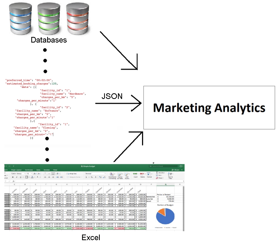
Figure 1.1: Data model of traditional marketing analytics
A data model with all these different kinds of data is prone to errors and is very risky to use. If we somehow get a garbage value into one of the attributes, our entire analysis will go awry. Most of the times, the data we need is of a certain kind and if we don't get that type of data, we might run into a bug or problem that would need to be investigated. Therefore, if we can enforce some checks to ensure that the data being passed to our model is almost always of the same kind, we can easily improve the quality of data from unstructured to at least semi-structured.
This is where programming languages such as Python come into play. Python is an all-purpose general programming language that not only makes writing structure-enforcing scripts easy, but also integrates with almost every platform and automates data production, analysis, and analytics into a more reliable and predictable pipeline. Apart from understanding patterns and giving at least a basic structure to data, Python forces intelligent pipelines to accept the right value for the right attribute. The majority of analytics pipelines are exactly of this kind. The following figure illustrates how most marketing analytics today structure different kinds of data by passing it through scripts to make it at least semi-structured:
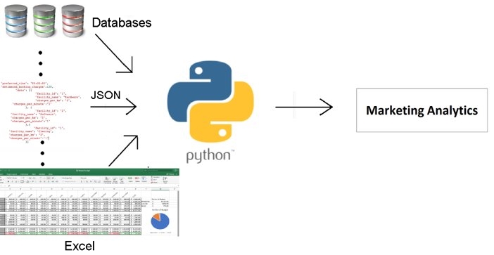
Figure 1.2: Data model of most marketing analytics that use Python
By making use of such structure-enforcing scripts, we will have a pipeline of semi-structured data coming in with expected values in the right fields; however, the data is not yet in the best possible format to perform analytics. If we can completely structure our data (that is, arrange it in flat tables, with the right value pointing to the right attribute with no nesting or hierarchy), it will be easy for us to see how every data point individually compares to other points being considered in the common fields, and would also make the pipeline scalable. We can easily get a feel of the data—that is, see in what range most values lie, identify the clear outliers, and so on—by simply scrolling through the data.
While there are a lot of tools that can be used to convert data from an unstructured/semi-structured format to a fully structured format (for example, Spark, STATA, and SAS), the tool that is most commonly used for data science, can be integrated with practically any framework, has rich functionalities, minimal costs, and is easy-to-use for our use case, is pandas. The following figure illustrates how a data model structures different kinds of data from being possibly unstructured to semi-structured (using Python), to completely structured (using pandas):
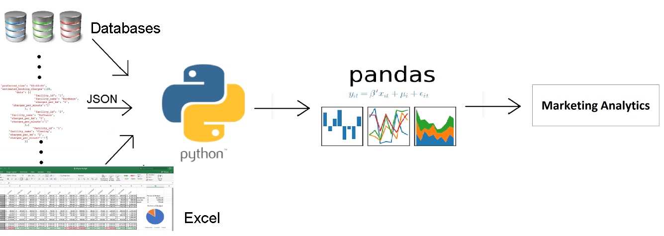
Figure 1.3: Data model to structure the different kinds of data
pandas is a software library written in Python and is the basis for data manipulation and analysis in the language. Its name comes from "panel data," an econometrics term for datasets that include observations over multiple time periods for the same individuals.
pandas offers a collection of high-performance, easy-to-use, and intuitive data structures and analysis tools that are of great use to marketing analysts and data scientists alike. It has the following two primary object types:
DataFrame: This is the fundamental tabular relationship object that stores data in rows and columns (like a spreadsheet). To perform data analysis, functions and operations can be directly applied to DataFrames.
Series: This refers to a single column of the DataFrame. The value can be accessed through its index. As Series automatically infers a type, it automatically makes all DataFrames well-structured.
The following figure illustrates a pandas DataFrame with an automatic integer index (0, 1, 2, 3...):
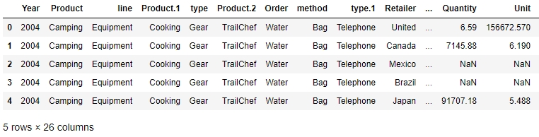
Figure 1.4: A sample pandas DataFrame
Now that we understand what pandas objects are and how they can be used to automatically get structured data, let's take a look at some of the functions we can use to import and export data in pandas and see if the data we passed is ready to be used for further analyses.
Every team in a marketing group can have its own preferred data type for their specific use case. Those who have to deal with a lot more text than numbers might prefer using JSON or XML, while others may prefer CSV, XLS, or even Python objects. pandas has a lot of simple APIs (application program interfaces) that allow it to read a large variety of data directly into DataFrames. Some of the main ones are shown here:
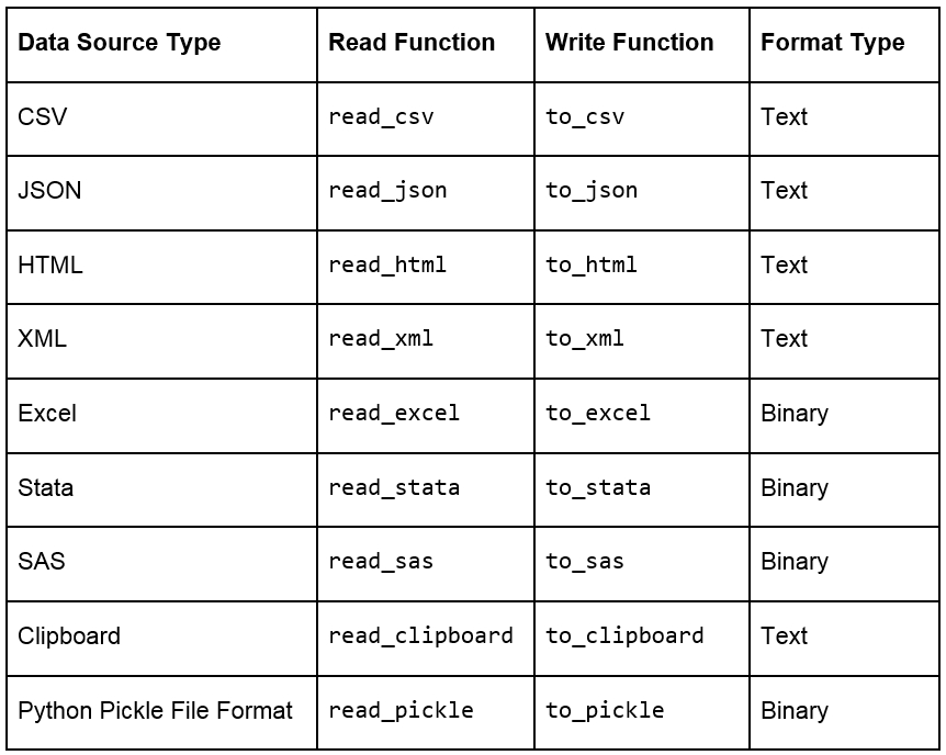
Figure 1.5: Ways to import and export different types of data with pandas DataFrames
Note
Remember that a well-structured DataFrame does not have hierarchical or nested data. The read_xml, read_json(), and read_html() functions (and others) cause the data to lose its hierarchical datatypes/nested structure and convert it into flattened objects such as lists and lists of lists. Pandas, however, does support hierarchical data for data analysis. You can save and load such data by pickling from your session and maintaining the hierarchy in such cases. When working with data pipelines, it's advised to split nested data into separate streams to maintain the structure.
When loading data, pandas provides us with additional parameters that we can pass to read functions, so that we can load the data differently. Some additional parameters that are used commonly when importing data into pandas are given here:
skiprows = k: This skips the first k rows.
nrows = k: This parses only the first k rows.
names = [col1, col2...]: This lists the column names to be used in the parsed DataFrame.
header = k: This applies the column names corresponding to the kth row as the header for the DataFrame. k can also be None.
index_col = col: This sets col as the index of the DataFrame being used. This can also be a list of column names (used to create a MultiIndex) or None.
usecols = [l1, l2...]: This provides either integer positional indices in the document columns or strings that correspond to column names in the DataFrame to be read. For example, [0, 1, 2] or ['foo', 'bar', 'baz'].
Once you've read the DataFrame using the API, as explained earlier, you'll notice that, unless there is something grossly wrong with the data, the API generally never fails, and we always get a DataFrame object after the call. However, we need to inspect the data ourselves to check whether the right attribute has received the right data, for which we can use several in-built functions that pandas provides. Assume that we have stored the DataFrame in a variable called df then:
df.head(n) will return the first n rows of the DataFrame. If no n is passed, by default, the function considers n to be 5.
df.tail(n) will return the last n rows of the DataFrame. If no n is passed, by default, the function considers n to be 5.
df.shape will return a tuple of the type (number of rows, number of columns).
df.dtypes will return the type of data in each column of the pandas DataFrame (such as float, char, and so on).
df.info() will summarize the DataFrame and print its size, type of values, and the count of non-null values.
For this exercise, you need to use the user_info.json file provided to you in the Lesson01 folder. The file contains some anonymous personal user information collected from six customers through a web-based form in JSON format. You need to open a Jupyter Notebook, import the JSON file into the console as a pandas DataFrame, and see whether it has loaded correctly, with the right values being passed to the right attribute.
Note
All the exercises and activities in this chapter can be done in both the Jupyter Notebook and Python shell. While we can do them in the shell for now, it is highly recommended to use the Jupyter Notebook. To learn how to install Jupyter and set up the Jupyter Notebook, check https://jupyter.readthedocs.io/en/latest/install.html. It will be assumed that you are using a Jupyter Notebook from the next chapter onward.
Note
The 64 displayed with the type above is an indicator of precision and varies on different platforms.
Open a Jupyter Notebook to implement this exercise. Once you are in the console, import the pandas library using the import command, as follows:
import pandas as pd
Read the user_info.json JSON file into the user_info DataFrame:
user_info = pd.read_json("user_info.json")Check the first few values in the DataFrame using the head command:
user_info.head()
You should see the following output:
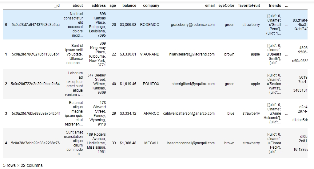
Figure 1.6: Viewing the first few rows of user_info.json
As we can see, the data makes sense superficially. Let's see if the data types match too. Type in the following command:
user_info.info()
You should get the following output:
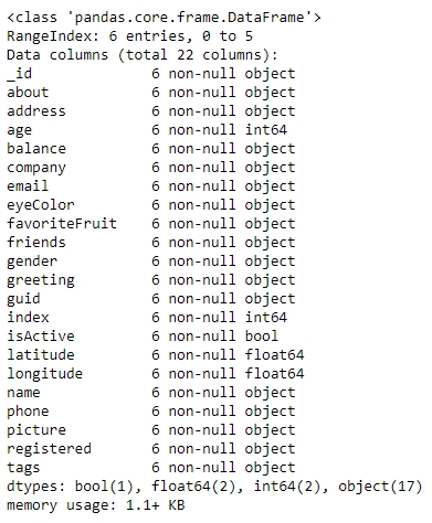
Figure 1.7: Information about the data in user_info
From the preceding figure, notice that the isActive column is Boolean, the age and index columns are integers, whereas the latitude and longitude columns are floats. The rest of the elements are Python objects, most likely to be strings. Looking at the names, they match our intuition. So, the data types seem to match. Also, the number of observations seems to be the same for all fields, which implies that there has been no data loss.
Let's also see the number of rows and columns in the DataFrame using the shape attribute of the DataFrame:
user_info.shape
This will give you (6, 22) as the output, indicating that the DataFrame created by the JSON has 6 rows and 22 columns.
Congratulations! You have loaded the data correctly, with the right attributes corresponding to the right columns and with no missing values. Since the data was already structured, it is now ready to be put into the pipeline to be used for further analysis.
In this exercise, you will be using the data.csv and sales.xlsx files provided to you in the Lesson01 folder. The data.csv file contains the views and likes of 100 different posts on Facebook in a marketing campaign, and sales.xlsx contains some historical sales data recorded in MS Excel about different customer purchases in stores in the past few years. We want to read the files into pandas DataFrames and check whether the output is ready to be added into the analytics pipeline. Let's first work with the data.csv file:
Import pandas into the console, as follows:
import pandas as pd
Use the read_csv method to read the data.csv CSV file into a campaign_data DataFrame:
campaign_data = pd.read_csv("data.csv")Look at the current state of the DataFrame using the head function:
campaign_data.head()
Your output should look as follows:
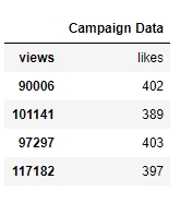
Figure 1.8: Viewing raw campaign_data
From the preceding output, we can observe that the first column has an issue; we want to have "views" and "likes" as the column names and for the DataFrame to have numeric values.
We will read the data into campaign_data again, but this time making sure that we use the first row to get the column names using the header parameter, as follows:
campaign_data = pd.read_csv("data.csv", header = 1)Let's now view campaign_data again, and see whether the attributes are okay now:
campaign_data.head()
Your DataFrame should now appear as follows:
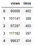
Figure 1.9: campaign_data after being read with the header parameter
The values seem to make sense—with the views being far more than the likes—when we look at the first few rows, but because of some misalignment or missing values, the last few rows might be different. So, let's have a look at it:
campaign_data.tail()
You will get the following output:
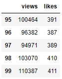
Figure 1.10: The last few rows of campaign_data
There doesn't seem to be any misalignment of data or missing values at the end. However, although we have seen the last few rows, we still can't be sure that all values in the middle (hidden) part of the DataFrame are okay too. We can check the datatypes of the DataFrame to be sure:
campaign_data.info()
You should get the following output:
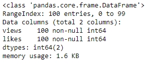
Figure 1.11: info() of campaign_data
We also need to ensure that we have not lost some observations because of our cleaning. We use the shape function for that:
campaign_data.shape
You will get an output of (100, 2), indicating that we still have 100 observations with 2 columns. The dataset is now completely structured and can easily be a part of any further analysis or pipeline.
Let's now analyze the sales.xlsx file. Use the read_excel function to read the file in a DataFrame called sales:
sales = pd.read_excel("sales.xlsx")Look at the first few rows of the sales DataFrame:
sales.head()
Your output should look as follows:

Figure 1.12: First few rows of sales.xlsx
From the preceding figure, the Year column appears to have matched to the right values, but the line column does not seem to make much sense. The Product.1, Product.2, columns imply that there are multiple columns with the same name! Even the values of the Order and method columns being Water and Bag, respectively, make us feel as though something is wrong.
Let's look at gathering some more information, such as null values and the data types of the columns, and see if we can make more sense of the data:
sales.info()
Your output will look as follows:
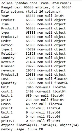
Figure 1.13: Output of sales.info()
As there are some columns with no non-null values, the column names seem to have broken up incorrectly. This is probably why the output of info showed a column such as revenue as having an arbitrary data type such as object (usually used to refer to columns containing strings). It makes sense if the actual column names start with a capital letter and the remaining columns are created as a result of data spilling from the preceding columns.
Let's try to read the file with just the new, correct column names and see whether we get anything. Use the following code:
sales = pd.read_excel("sales.xlsx", names = ["Year", "Product line", "Product type", "Product", "Order method type", "Retailer Country", "Revenue", "Planned revenue", "Product cost", "Quantity", "Unit cost", "Unit price", "Gross Profit", "Unit sale price"])You get the following output:
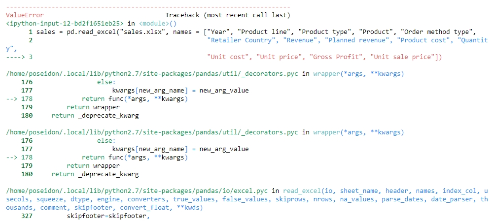
Figure 1.14: Attempting to structure sales.xlsx
Unfortunately, the issue is not just with the columns, but with the underlying values too. The value of one column is leaking into another and thus ruining the structure. Understandably, the code fails because of length mismatch. Therefore, we can conclude that the sales.xlsx data is very unstructured.
With the use of the API and what we know up till this point, we can't directly get this data to be structured. To understand how to approach structuring this kind of data, we need to dive deep into the internal structure of pandas objects and understand how data is actually stored in pandas, which we will do in the following sections. We will come back to preparing this data for further analysis in a later section.
Let's say you want to store some values from a data store in a data structure. It is not necessary for every element of the data to have values, so your structure should be able to handle that. It is also a very common scenario where there is some discrepancy between two data sources on how to identify a data point. So, instead of using default numerical indices (such as 0-100) or user-given names to access it, like in a dictionary, you would like to access every value by a name that comes from within the data source. This is achieved in pandas using a pandas Series.
A pandas Series is nothing but an indexed NumPy array. To make a pandas Series, all you need to do is create an array and give it an index. If you create a Series without an index, it will create a default numeric index that starts from 0 and goes on for the length of the Series, as shown in the following figure:
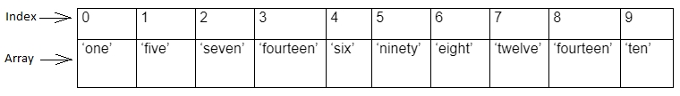
Figure 1.15: Sample pandas Series
Note
As a Series is still a NumPy array, all functions that work on a NumPy array, work the same way on a pandas Series too.
Once you've created a number of Series, you might want to access the values associated with some specific indices all at once to perform an operation. This is just aggregating the Series with a specific value of the index. It is here that pandas DataFrames come into the picture. A pandas DataFrame is just a dictionary with the column names as keys and values as different pandas Series, joined together by the index:
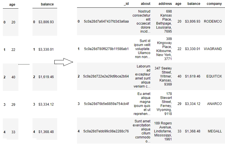
Figure 1.16: Series joined together by the same index create a pandas Dataframe
This way of storing data makes it very easy to perform the operations we need on the data we want. We can easily choose the Series we want to modify by picking a column and directly slicing off indices based on the value in that column. We can also group indices with similar values in one column together and see how the values change in other columns.
Other than this one-dimensional Series structure to access the DataFrame, pandas also has the concept of axes, where an operation can be applied to both rows (or indices) and columns. You can choose which one to apply it to by specifying the axis, 0 referring to rows and 1 referring to columns, thereby making it very easy to access the underlying headers and the values associated with them:
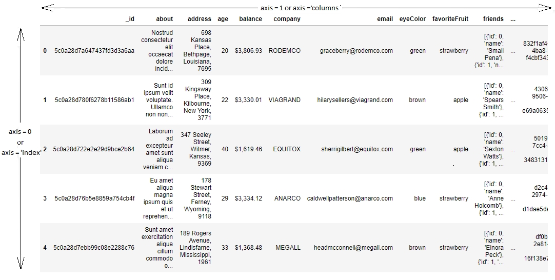
Figure 1.17: Understanding axis = 0 and axis = 1 in pandas
Now that we have deconstructed the structure of the pandas DataFrame down to its basics, the rest of the wrangling tasks, that is, creating new DataFrames, selecting or slicing a DataFrame into its parts, filtering DataFrames for some values, joining different DataFrames, and so on, will become very intuitive.
It is standard convention in spreadsheets to address a cell by (column name, row name). Since data is stored in pandas in a similar manner, this is also the way to address a cell in a pandas DataFrame: the column name acts as a key to give you the pandas Series, and the row name gives you the value on that index of the DataFrame.
But if you need to access more than a single cell, such as a subset of some rows and columns from the DataFrame, or change the order of display of some columns on the DataFrame, you can make use of the syntax listed in the following table:
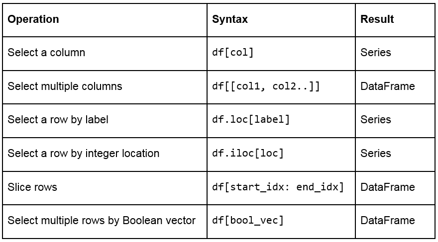
Figure 1.18: A table listing the syntax used for different operations on a pandas DataFrame
We frequently need to create test objects while building a data pipeline in pandas. Test objects give us a reference point to figure out what we have been able to do up till that point and make it easier to debug our scripts. Generally, test DataFrames are small in size, so that the output of every process is quick and easy to compute. There are two ways to create test DataFrames—by creating completely new DataFrames, or by duplicating or taking a slice of a previously existing DataFrame:
Creating new DataFrames: We typically use the DataFrame method to create a completely new DataFrame. The function directly converts a Python object into a pandas DataFrame. The DataFrame function will, in general, work with any iterable collection of data (such as dict, list, and so on). We can also pass an empty collection or a singleton collection to the function.
For example, we will get the same DataFrame through either of the following lines of code:
pd.DataFrame({'category': pd.Series([1, 2, 3])}
pd.DataFrame([1, 2, 3], columns=['category'])
pd.DataFrame.from_dict({'category': [1, 2, 3]})
The following figure shows the outputs received each time:
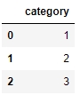
Figure 1.19: Output generated by all three ways to create a DataFrame
A DataFrame can also be built by passing any pandas objects to the DataFrame function. The following line of code gives the same output as the preceding figure:
pd.DataFrame(pd.Series([1,2,3]), columns=["category"])
Duplicating or slicing a previously existing DataFrame: The second way to create a test DataFrame is by copying a previously existing DataFrame. Python, and therefore, pandas, has shallow references. When we say obj1 = obj2, the objects share the location or the reference to the same object in memory. So, if we change obj2, obj1 also gets modified, and vice versa. This is tackled in the standard library with the deepcopy function in the copy module. The deepcopy function allows the user to recursively go through the objects being pointed to by the references and create entirely new objects.
So, when you want to copy a previously existing DataFrame and don't want the previous DataFrame to be affected by modifications in the current DataFrame, you need to use the deepcopy function. You can also slice the previously existing DataFrame and pass it to the function, and it will be considered a new DataFrame. For example, the following code snippet will recursively copy everything in df1 and not have any references to it when you make changes to df:
import pandas
import copy
df = copy.deepcopy(df1)
pandas provides the following functions to add and delete rows (observations) and columns (attributes):
df['col'] = s: This adds a new column, col, to the DataFrame, df, with the Series, s.
df.assign(c1 = s1, c2 = s2...): This adds new columns, c1, c2, and so on, with series, s1, s2, and so on, to the df DataFrame in one go.
df.append(df2 / d2, ignore_index): This adds values from the df2 DataFrame to the bottom of the df DataFrame wherever the columns of df2 match those of df. Alternatively, it also accepts dict and d2, and if ignore_index = True, it does not use index labels.
df.drop(labels, axis): This remove the rows or columns specified by the labels and corresponding axis, or those specified by the index or column names directly.
df.dropna(axis, how): Depending on the parameter passed to how, this decides whether to drop rows (or columns if axis = 1) with missing values in any of the fields or in all of the fields. If no parameter is passed, the default value of how is any and the default value of axis is 0.
df.drop_duplicates(keep): This removes rows with duplicate values in the DataFrame, and keeps the first (keep = 'first'), last (keep = 'last'), or no occurrence (keep = False) in the data.
We can also combine different pandas DataFrames sequentially with the concat function, as follows:
pd.concat([df1,df2..]): This creates a new DataFrame with df1, df2, and all other DataFrames combined sequentially. It will automatically combine columns having the same names in the combined DataFrames.
This exercise aims to test the understanding of the students about creating and modifying DataFrames in pandas. We will create a test DataFrame from scratch and add and remove rows/columns to it by making use of the functions and concepts described so far:
Import pandas and copy libraries that we will need for this task (the copy module in this case):
import pandas as pd
import copy
Create a DataFrame, df1, and use the head method to see the first few rows of the DataFrame. Use the following code:
df1 = pd.DataFrame({'category': pd.Series([1, 2, 3])})
df1.head()
Your output should be as follows:
Figure 1.20: The first few rows of df1
Create a test DataFrame, df, by duplicating df1. Use the deepcopy function:
df = copy.deepcopy(df1)
df.head()
You should get the following output:
Figure 1.21: The first few rows of df
Add a new column, cities, containing different kinds of city groups to the test DataFrame using the following code and take a look at the DataFrame again:
df['cities'] = pd.Series([['Delhi', 'Mumbai'], ['Lucknow', 'Bhopal'], ['Chennai', 'Bangalore']])
df.head()
You should get the following output:
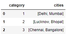
Figure 1.22: Adding a row to df
Now, add multiple columns pertaining to the user viewership using the assign function and again look at the data. Use the following code:
df.assign(
    young_viewers = pd.Series([2000000, 3000000, 1500000]),
    adult_viewers = pd.Series([2500000, 3500000, 1600000]),
    aged_viewers = pd.Series([2300000, 2800000, 2000000])
)
df.head()
Your DataFrame will now appear as follows:
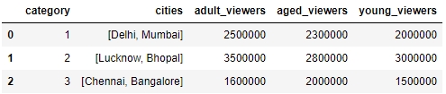
Figure 1.23: Adding multiple columns to df
Use the append function to add a new row to the DataFrame. As we know that the new row contains partial information, we will pass the ignore_index parameter as True:
df.append({'cities': ["Kolkata", "Hyderabad"], 'adult_viewers': 2000000,
   'aged_viewers': 2000000, 'young_viewers': 1500000}, ignore_index = True)
df.head()
Your DataFrame should now look as follows:
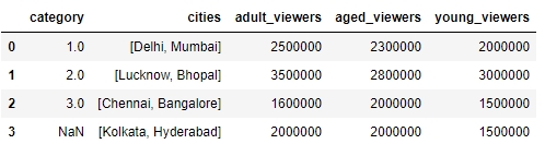
Figure 1.24: Adding another row by using the append function on df
Now, use the concat function to duplicate the test DataFrame and save it as df2. Take a look at the new DataFrame:
df2 = pd.concat([df, df], sort = False)
df2
df2 will show duplicate entries of df1, as shown here:
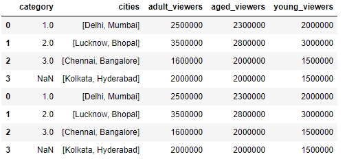
Figure 1.25: Using the concat function to duplicate a DataFrame, df2, in pandas
To delete a row from the df DataFrame, we will now pass the index of the row we want to delete—in this case, the third row—to the drop function, as follows:
df.drop([3])
You will get the following output:
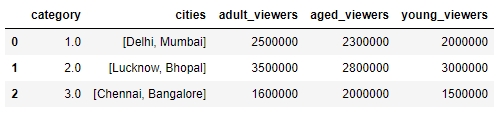
Figure 1.26: Using the drop function to delete a row
Similarly, let's delete the aged_viewers column from the DataFrame. We will pass the column name as the parameter to the drop function and specify the axis as 1:
df.drop(['aged_viewers'])
Your output will be as follows:
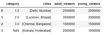
Figure 1.27: Dropping the aged_viewers column in the DataFrame
Note that, as the result of the drop function is also a DataFrame, we can chain another function on it too. So, we drop the cities field from df2 and remove the duplicates in it as well:
df2.drop('cities', axis = 1).drop_duplicates()The df2 DataFrame will now look as follows:
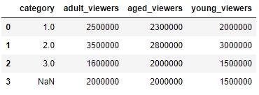
Figure 1.28: Dropping the cities field and then removing duplicates in df2
Congratulations! You've successfully performed some basic operations on a DataFrame. You now know how to add rows and columns to DataFrames and how to concatenate multiple DataFrames together in a big DataFrame.
In the next section, you will learn how to combine multiple data sources into the same DataFrame. When combining data sources, we need to make sure to include common columns from both sources but make sure that no duplication occurs. We would also need to make sure that, unlike the concat function, the combined DataFrame is smart about the index and does not duplicate rows that already exist. This feature is also covered in the next section.
Once the data is prepared from multiple sources in separate pandas DataFrames, we can use the pd.merge function to combine them into the same DataFrame based on a relevant key passed through the on parameter. It is possible that the joining key is named differently in the different DataFrames that are being joined. So, while calling pd.merge(df, df1), we can provide a left_on parameter to specify the column to be merged from df and a right_on parameter to specify the index in df1.
pandas provides four ways of combining DataFrames through the how parameter. All values of these are different joins by themselves and are described as follows:
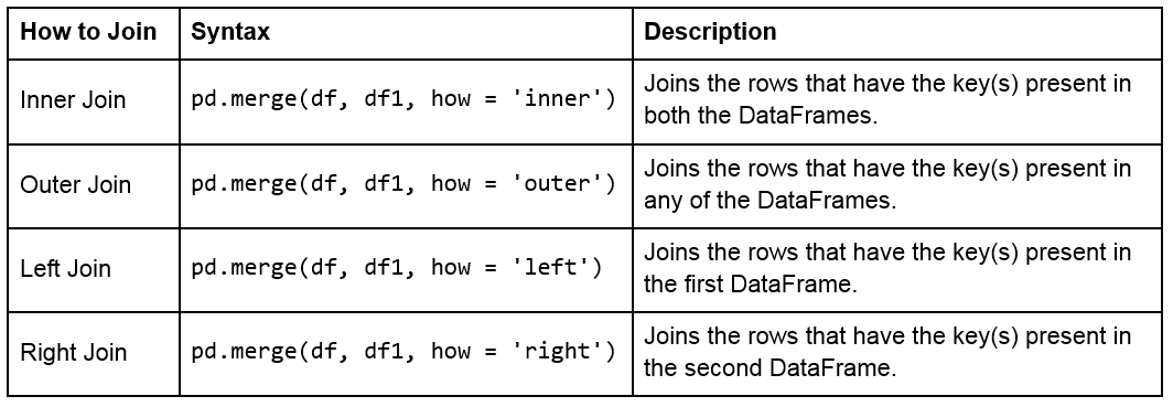
Figure 1.29: Table describing different joins
The following figure shows two sample DataFrames, df1 and df2, and the results of the various joins performed on these DataFrames:

Figure 1.30: Table showing two DataFrames and the outcomes of different joins on them
For example, we can perform a right and outer join on the DataFrames of the previous exercise using the following code:
pd.merge(df, df1, how = 'right')
pd.merge(df, df1, how = 'outer')
The following will be the output of the preceding two joins:
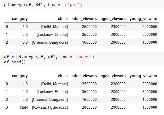
Figure 1.31: Examples of the different types of merges in pandas
Once we have joined two datasets, it is easy to see what happens to an index present in one of the tables but not in the other. The other columns of that index get the np.nan value, which is pandas' way of telling us that data is missing in that column. Depending on where and how the values are going to be used, missing values can be treated differently. The following are various ways of treating missing values:
We can get rid of missing values completely using df.dropna, as explained in the Adding and Removing Attributes and Observations section.
We can also replace all the missing values at once using df.fillna(). The value we want to fill in will depend heavily on the context and the use case for the data. For example, we can replace all missing values with the mean or median of the data, or even some easy to filter values, such as –1 using df.fillna(df.mean()),df.fillna(df.median), or df.fillna(-1), as shown here:
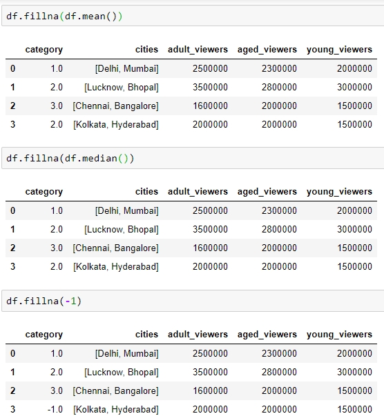
Figure 1.32: Using the df.fillna function
We can interpolate missing values using the interpolate function:
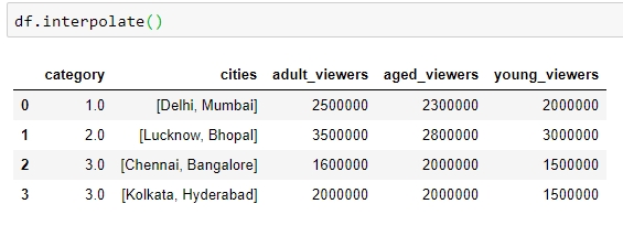
Figure 1.33: Using the interpolate function to predict category
Other than using in-built operations, we can also perform different operations on DataFrames by filtering out rows with missing values in the following ways:
We can check for slices containing missing values using the pd.isnull() function, or those without it using the pd.isnotnull() function, respectively:
df.isnull()
You should get the following output:
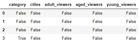
Figure 1.34: Using the .isnull function
We can check whether individual elements are NA using the isna function:
df[['category']].isna
This will give you the following output:
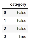
Figure 1.35: Using the isna function
This describes missing values only in pandas. You might come across different types of missing values in your pandas DataFrame if it gets data from different sources, for example, None in databases. You'll have to filter them out separately, as described in previous sections, and proceed.
The aim of this exercise is to get you used to combining different DataFrames and handling missing values in different contexts, as well as to revisit how to create DataFrames. The context is to get user information about users definitely watching a certain webcast on a website so that we can recognize patterns in their behavior:
Import the numpy and pandas modules, which we'll be using:
importnumpy as np
import pandas as pd
Create two empty DataFrames, df1 and df2:
df1 = pd.DataFrame()
df2 = pd.DataFrame()
We will now add dummy information about the viewers of the webcast in a column named viewers in df1, and the people using the website in a column named users in df2. Use the following code:
df1['viewers'] = ["Sushmita", "Aditya", "Bala", "Anurag"]
df2['users'] = ["Aditya", "Anurag", "Bala", "Sushmita", "Apoorva"]
We will also add a couple of additional columns to each DataFrame. The values for these can be added manually or sampled from a distribution, such as normal distribution through NumPy:
np.random.seed(1729)
df1 = df1.assign(views = np.random.normal(100, 100, 4))
df2 = df2.assign(cost = [20, np.nan, 15, 2, 7])
View the first few rows of both DataFrames, still using the head method:
df1.head()
df2.head()
You should get the following outputs for both df1 and df2:
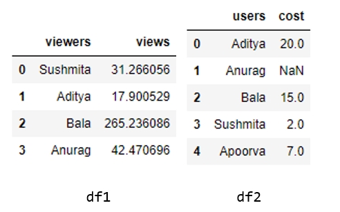
Figure 1.36: Contents of df1 and df2
Do a left join of df1 with df2 and store the output in a DataFrame, df, because we only want the user stats in df2 of those users who are viewing the webcast in df1. Therefore, we also specify the joining key as "viewers" in df1 and "users" in df2:
df = df1.merge(df2, left_on="viewers", right_on="users", how="left")
df.head()
Your output should now look as follows:
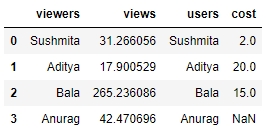
Figure 1.37: Using the merge and fillna functions
You'll observe some missing values (NaN) in the preceding output. We will handle these values in the DataFrame by replacing them with the mean values in that column. Use the following code:
df.fillna(df.mean())
Your output will now look as follows:
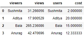
Figure 1.38: Imputing missing values with the mean through fillna
Congratulations! You have successfully wrangled with data in data pipelines and transformed attributes externally. But to handle the sales.xlsx file that we saw previously, this is still not enough. We need to apply functions and operations on the data inside the DataFrame too. Let's learn how to do that and more in the next section.
By default, operations on all pandas objects are element-wise and return the same type of pandas objects. For instance, look at the following code:
df['viewers'] = df['adult_viewers']+df['aged_viewers']+df['young_viewers']
This will add a viewers column to the DataFrame with the value for each observation being equal to the sum of the values in the adult_viewers, aged_viewers, and young_viewers columns.
Similarly, the following code will multiply every numerical value in the viewers column of the DataFrame by 0.03 or whatever you want to keep as your target CTR (click-through rate):
df['expected clicks'] = 0.03*df['viewers']
Hence, your DataFrame will look as follows once these operations are performed:
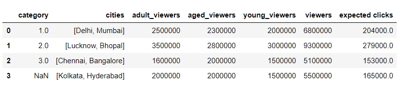
Figure 1.39: Operations on pandas DataFrames
Pandas also supports several out-of-the-box built-in functions on pandas objects. These are listed in the following table:
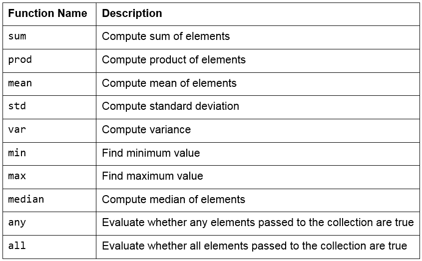
Figure 1.40: Built-in functions used in pandas
Note
Remember that pandas objects are Python objects too. Therefore, we can write our own custom functions to perform specific tasks on them.
We can iterate through the rows and columns of pandas objects using itertuples or iteritems. Consider the following DataFrame, named df:
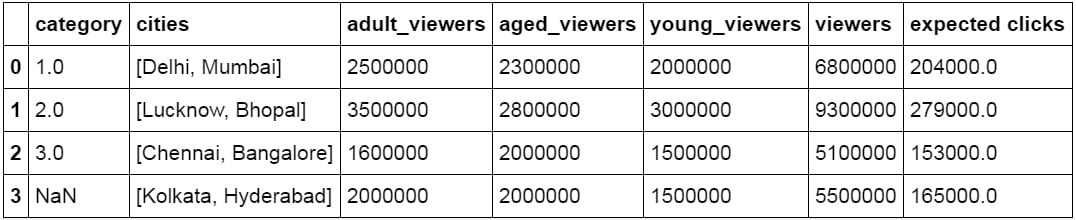
Figure 1.41: DataFrame df
The following methods can be performed on this DataFrame:
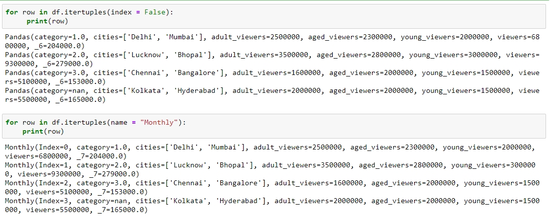
Figure 1.42: Testing itertuples
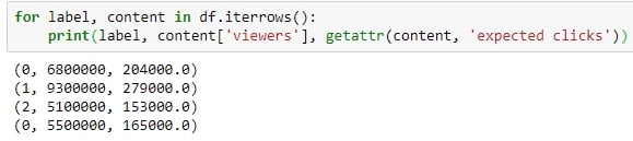
Figure 1.43: Testing iterrows
itertuples: This method iterates over the rows of the DataFrame in the form of named tuples. By setting the index parameter to False, we can remove the index as the first element of the tuple and set a custom name for the yielded named tuples by setting it in the name parameter. The following screenshot illustrates this over the DataFrame shown in the preceding figure:
iterrows: This method iterates over the rows of the DataFrame in tuples of the type (label, content), where label is the index of the row and content is a pandas Series containing every item in the row. The following screenshot illustrates this:
iteritems: This method iterates over the columns of the DataFrame in tuples of the type (label,content), where label is the name of the column and content is the content in the column in the form of a pandas Series. The following screenshot shows how this is performed:
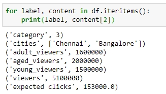
Figure 1.44: Checking out iteritems
To apply built-in or custom functions to pandas, we can make use of the map and apply functions. We can pass any built-in, NumPy, or custom functions as parameters to these functions, and they will be applied to all elements in the column:
map: This returns an object of the same kind as that was passed to it. A dictionary can also be passed as input to it, as shown here:
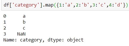
Figure 1.45: Using the map function
apply: This applies the function to the object passed and returns a DataFrame. It can easily take multiple columns as input. It also accepts the axis parameter, depending on how the function is to be applied, as shown:
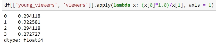
Figure 1.46: Using the apply function
Other than working on just DataFrames and Series, functions can also be applied to pandas GroupBy objects. Let's see how that works.
Suppose you want to apply a function differently on some rows of a DataFrame, depending on the values in a particular column in that row. You can slice the DataFrame on the key(s) you want to aggregate on and then apply your function to that group, store the values, and move on to the next group.
pandas provides a much better way to do this, using the groupby function, where you can pass keys for groups as a parameter. The output of this function is a DataFrameGroupBy object that holds groups containing values of all the rows in that group. We can select the new column we would like to apply a function to, and pandas will automatically aggregate the outputs on the level of different values on its keys and return the final DataFrame with the functions applied to individual rows.
For example, the following will collect the rows that have the same number of aged_viewers together, take their values in the expected clicks column, and add them together:
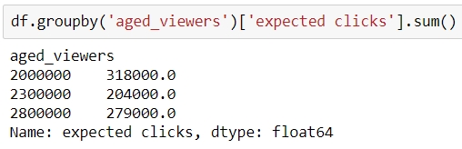
Figure 1.47: Using the groupby function on a Series
Instead, if we were to pass [['series']] to the GroupBy object, we would have gotten a DataFrame back, as shown:
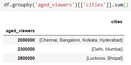
Figure 1.48: Using the groupby function on a DataFrame
The aim of this exercise is to get you used to performing regular and groupby operations on DataFrames and applying functions to them. You will use the user_info.json file in the Lesson02 folder on GitHub, which contains information about six customers.
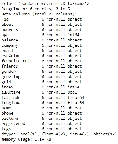
Figure 1.50: Output of the info function on user_info
Import the pandas module that we'll be using:
import pandas as pd
Read the user_info.json file into a pandas DataFrame, user_info, and look at the first few rows of the DataFrame:
user_info = pd.read_json('user_info.json')
user_info.head()
You will get the following output:
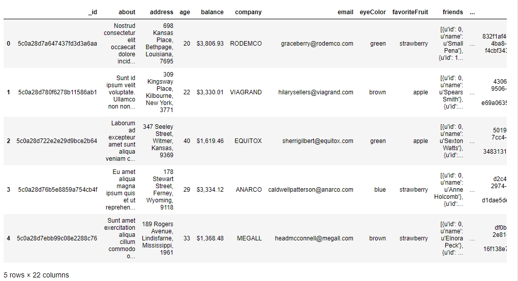
Figure 1.49: Output of the head function on user_info
Now, look at the attributes and the data inside them:
user_info.info()
You will get the following output:
Let's make use of the map function to see how many friends each user in the data has. Use the following code:
user_info['friends'].map(lambda x: len(x))
You will get the following output:
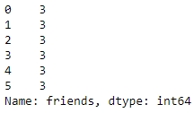
Figure 1.51: Using the map function on user_info
We use the apply function to get a grip on the data within each column individually and apply regular Python functions to it. Let's convert all the values in the tags column of the DataFrame to capital letters using the upper function for strings in Python, as follows:
user_info['tags'].apply(lambda x: [t.upper() for t in x])
You should get the following output:
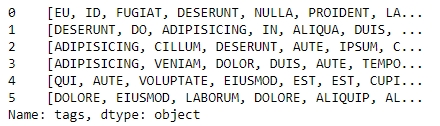
Figure 1.52: Converting values in tags
Use the groupby function to get the different values obtained by a certain attribute. We can use the count function on each such mini pandas DataFrame generated. We'll do this first for the eye color:
user_info.groupby('eyeColor')['_id'].count()Your output should now look as follows:
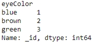
Figure 1.53: Checking distribution of eyeColor
Similarly, let's look at the distribution of another variable, favoriteFruit, in the data too:
user_info.groupby('favoriteFruit')['_id'].count()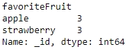
Figure 1.54: Seeing the distribution in use_info
We are now sufficiently prepared to handle any sort of problem we might face when trying to structure even unstructured data into a structured format. Let's do that in the activity here.
We will now solve the problem that we encountered in Exercise 1. We start by loading sales.xlsx, which contains some historical sales data, recorded in MS Excel, about different customer purchases in stores in the past few years. Your current team is only interested in the following product types: Climbing Accessories, Cooking Gear, First Aid, Golf Accessories, Insect Repellents, and Sleeping Bags. You need to read the files into pandas DataFrames and prepare the output so that it can be added into your analytics pipeline. Follow the steps given here:
Open the Python console and import pandas and the copy module.
Load the data from sales.xlsx into a separate DataFrame, named sales, and look at the first few rows of the generated DataFrame. You will get the following output:
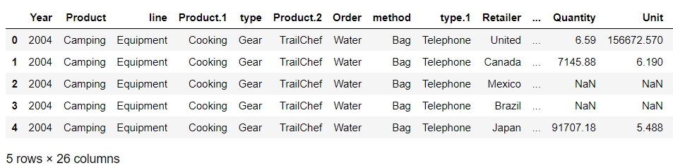
Figure 1.55: Output of the head function on sales.xlsx
Analyze the datatype of the fields and get hold of prepared values.
Get the column names right. In this case, every new column starts with a capital case.
Look at the first column, if the value in the column matches the expected values, just correct the column name and move on to the next column.
Take the first column with values leaking into other columns and look at the distribution of its values. Add the values from the next column and go on to as many columns as required to get to the right values for that column.
Slice out the portion of the DataFrame that has the largest number of columns required to cover the value for the right column and structure the values for that column correctly in a new column with the right attribute name.
You can now drop all the columns from the slice that are no longer required once the field has the right values and move on to the next column.
Repeat 4–7 multiple times, until you have gotten a slice of the DataFrame completely structured with all the values correct and pointing to the intended column. Save this DataFrame slice. Your final structured DataFrame should appear as follows:
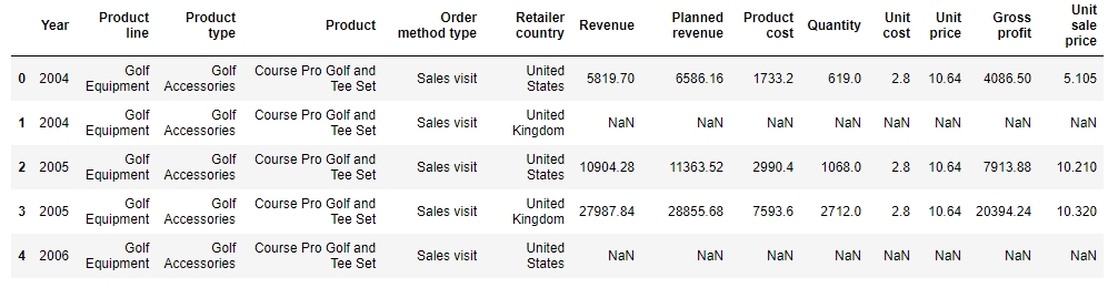
Figure 1.56: First few rows of the structured DataFrame
Data processing and wrangling is the initial, and a very important, part of the data science pipeline. It is generally helpful if people preparing data have some domain knowledge about the data, since that will help them stop at the right processing point and use their intuition to build the pipeline better and more quickly. Data processing also requires coming up with innovative solutions and hacks.
In this chapter, you learned how to structure large datasets by arranging them in a tabular form. Then, we got this tabular data into pandas and distributed it between the right columns. Once we were sure that our data was arranged correctly, we combined it with other data sources. We also got rid of duplicates and needless columns, and finally, dealt with missing data. After performing these steps, our data was made ready for analysis and could be put into a data science pipeline directly.
In the next chapter, we will deepen our understanding of pandas and talk about reshaping and analyzing DataFrames for better visualizations and summarizing data. We will also see how to directly solve generic business-critical problems efficiently.