


 Download code from GitHub
In this first chapter, we are going to build the solid foundations so we can go through the following chapters easily. The topics we are going to discuss in this chapter are:
To follow along with this chapter including the source code, we require the following:
- A desktop PC or Notebook with Windows, Linux, or macOS
- GNU GCC v5.4.0 or above
- Code::Block IDE v17.12 (for Windows and Linux OS) or Code::Block IDE v13.12 (for macOS)
- You will find the code files on GitHub—https://github.com/PacktPublishing/CPP-Data-Structures-and-Algorithms
Before we go through the data structures and algorithms in C++, we need to have a strong, fundamental understanding of the language itself. In this section, we are going to build a simple program, build it, and then run it. We are also going to discuss the fundamental and advanced data types, and before we move on to algorithm analysis, we are going to discuss control flow in this section.
In C++, the code is executed from the main() function first. The function itself is a collection of statements to perform a specific task. As a result of this, a program in C++ has to contain at least one function named main(). The following code is the simplest program in C++ that will be successfully compiled and run:
    int main()
    {
      return 0;
    }
Suppose the preceding code is saved as a simple.cpp file. We can compile the code using the g++ compiler by running the following compiling command on the console from the active directory where the simple.cpp file is placed:
g++ simple.cppIf no error message appears, the output file will be generated automatically. If we run the preceding compiling command on a Windows console, we will get a file named a.exe. However, if we run the command on Bash shells, such as Linux or macOS, we will get a file named a.out.
We can specify the output file name using the -o option followed by the desired filename. For instance, the following compiling command will produce the output file named simple.out:
g++ simple.cpp -o simple.outIndeed, when we run the output file (by typing a and then pressing Enter on a Windows console or by typing ./a.out and then pressing Enter on Bash shell), we won't see anything on the console window. This is because we don't print anything to the console yet. To make our simple.cpp file meaningful, let's refactor the code so that it can receive the input data from the user and then print the data back to the user. The refactored code should look as follows:
    // in_out.cpp
    #include <iostream>

    int main ()
    {
      int i;
      std::cout << "Please enter an integer value: ";
      std::cin >> i;
      std::cout << "The value you entered is " << i;
      std::cout << "\n";
      return 0;
   }
As we can see in the preceding code, we appended several lines of code so that the program can print to the console and the user can give an input to the program. Initially, the program displays text that asks the user to input an integer number. After the user types the desired number and presses Enter, the program will print that number. We also defined a new variable named i of the int data type. This variable is used to store data in an integer data format (we will talk about variables and data types in the upcoming section).
Suppose we save the preceding code as in_out.cpp; we can compile it using the following command:
g++ in_out.cppIf we then run the program, we will get the following output on the console (I chose the number 3 in this example):
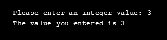
Now, we know that to print text to the console, we use the std::cout command, and to give some inputs to the program, we use the std::cin command. In the in_out.cpp file, we also see #include <iostream> at the beginning of the file. It's used to tell the compiler where to find the implementation of the std::cout and std::cin commands since their implementation is stated in the iostream header file.
And at the very beginning of the file, we can see that the line begins with double slashes (//). This means that the line won't be considered as code, so the compiler will ignore it. It's used to comment or mark an action in the code so that other programmers can understand our code.
So far, we have been able to create a C++ code, compile the code, and run the code. However, it will be boring if we have to compile the code using the Command Prompt and then execute the code afterwards. To ease our development process, we will use an integrated development environment (IDE) so that we can compile and run the code with just a click. You can use any C++ IDE available on the market, either paid or free. However, I personally chose Code::Blocks IDE since it's free, open source, and cross-platform so it can run on Windows, Linux, and macOS machines. You can find the information about this IDE, such as how to download, install, and use it on its official website at http://www.codeblocks.org/.
Actually, we can automate the compiling process using a toolchain such as Make or CMake. However, this needs further explanation, and since this book is intended to discuss data structures and algorithms, the toolchain explanation will increase the total pages of the book, and so we will not discuss this here. In this case, the use of IDE is the best solution to automate the compiling process since it actually accesses the toolchain as well.
After installing Code::Blocks IDE, we can create a new project by clicking on the File menu, then clicking New, and then selecting Project. A new window will appear and we can select the desired project type. For most examples in this book, we will use the Console Application as the project type. Press the Go button to continue.
On the upcoming window, we can specify the language, which is C++, and then define the project name and destination location (I named the project FirstApp). After finishing the wizard, we will have a new project with a main.cpp file containing the following code:
    #include <iostream>

    using namespace std;

    int main()
    {
      cout << "Hello world!" << endl;
      return 0;
    }
Now, we can compile and run the preceding code by just clicking the Build and run option under the Build menu. The following console window will appear:
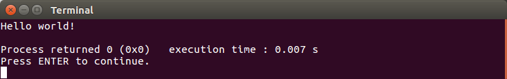
In the preceding screenshot, we see the console using namespace std in the line after the #include <iostream> line. The use of this line of code is to tell the compiler that the code uses a namespace named std. As a result, we don't need to specify the std:: in every invocation of the cin and cout commands. The code should be simpler than before.
In the previous sample codes, we dealt with the variable (a placeholder is used to store a data element) so that we can manipulate the data in the variable for various operations. In C++, we have to define a variable to be of a specific data type so it can only store the specific type of variable that was defined previously. Here is a list of the fundamental data types in C++. We used some of these data types in the previous example:
- Boolean data type (
bool), which is used to store two pieces of conditional data only—trueorfalse - Character data type (
char,wchar_t,char16_t, andchar32_t), which is used to store a single ASCII character - Floating point data type (
float,double, andlong double), which is used to store a number with a decimal - Integer data type (
short,int,long, andlong long), which is used to store a whole number - No data (
void), which is basically a keyword to use as a placeholder where you would normally put a data type to represent no data
There are two ways to create a variable—by defining it or by initializing it. Defining a variable will create a variable without deciding upon its initial value. The initializing variable will create a variable and store an initial value in it. Here is the code snippet for how we can define variables:
    int iVar;
    char32_t cVar;
    long long llVar;
    bool boVar;
And here is the sample code snippet of how initializing variables works:
    int iVar = 100;
    char32_t cVar = 'a';
    long long llVar = 9223372036854775805;
    bool boVar = true;
The preceding code snippet is the way we initialize the variables using the copy initialization technique. In this technique, we assign a value to the variable using an equals sign symbol (=). Another technique we can use to initialize a variable is the direct initialization technique. In this technique, we use parenthesis to assign a value to the variable. The following code snippet uses this technique to initialize the variables:
    int iVar(100);
    char32_t cVar('a');
    long long llVar(9223372036854775805);
    bool boVar(true);
Besides copy initialization and direct initialization techniques, we can use uniform initialization by utilizing curly braces. The following code snippet uses the so-called brace-initialization technique to initialize the variables:
    int iVar{100};
    char32_t cVar{'a'};
    long long llVar{9223372036854775805};
    bool boVar{true};
We cannot define a variable with a void data type such as void vVar because when we define a variable, we have to decide what data type we are choosing so that we can store the data in the variable. If we define a variable as void, it means that we don't plan to store anything in the variable.
As we discussed earlier, the C++ program is run from the main() function by executing each statement one by one from the beginning to the end. However, we can change this path using flow control statements. There are several flow control statements in C++, but we are only going to discuss some of them, since these are the ones that are going to be used often in algorithm design.
One of the things that can make the flow of a program change is a conditional statement. By using this statement, only the line in the true condition will be run. We can use the if and else keywords to apply this statement.
Let's modify our previous in_out.cpp code so that it uses the conditional statement. The program will only decide whether the input number is greater than 100 or not. The code should be as follows:
    // If.cbp
    #include <iostream>

    using namespace std;

    int main ()
    {
      int i;
      cout << "Please enter an integer value: ";
      cin >> i;
      cout << "The value you entered is ";

      if(i > 100)
         cout << "greater than 100.";
      else
         cout << "equals or less than 100.";

      cout << endl;
      return 0;
    }
As we can see, we have a pair of the if and else keywords that will decide whether the input number is greater than 100 or not. By examining the preceding code, only one statement will be executed inside the conditional statement, either the statement under the if keyword or the statement under the else keyword.
If we build and run the preceding code, we will see the following console window:
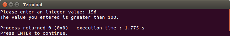
From the preceding console window, we can see that the line std::cout << "equals or less than 100."; is not executed at all since we have input a number that is greater than 100.
Also, in the if...else condition, we can have more than two conditional statements. We can refactor the preceding code so that it has more than two conditional statements, as follows:
    // If_ElseIf.cbp
    #include <iostream>

    using namespace std;

   int main ()
   {
      int i;
      cout << "Please enter an integer value: ";
      cin >> i;
      cout << "The value you entered is ";

      if(i > 100)
          cout << "greater than 100.";
      else if(i < 100)
          cout << "less than 100.";
      else
          cout << "equals to 100";

      cout << endl;
      return 0;
   }
Another conditional statement keyword is switch. Before we discuss this keyword, let's create a simple calculator program that can add two numbers. It should also be capable of performing the subtract, multiply, and divide operations. We will use the if...else keyword first. The code should be as follows:
// If_ElseIf_2.cbp
#include <iostream>
using namespace std;
int main ()
{
int i, a, b;
cout << "Operation Mode: " << endl;
cout << "1. Addition" << endl;
cout << "2. Subtraction" << endl;
cout << "3. Multiplication" << endl;
cout << "4. Division" << endl;
cout << "Please enter the operation mode: ";
cin >> i;
cout << "Please enter the first number: ";
cin >> a;
cout << "Please enter the second number: ";
cin >> b;
cout << "The result of ";
if(i == 1)
cout << a << " + " << b << " is " << a + b;
else if(i == 2)
cout << a << " - " << b << " is " << a - b;
else if(i == 3)
cout << a << " * " << b << " is " << a * b;
else if(i == 4)
cout << a << " / " << b << " is " << a / b;
cout << endl;
return 0;
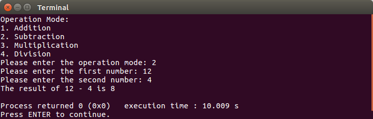
}As we can see in the preceding code, we have four options that we have to choose from. We use the if...else conditional statement for this purpose. The output of the preceding code should be as follows:
However, we can use the switch keyword as well. The code should be as follows after being refactored:
    // Switch.cbp
    #include <iostream>

    using namespace std;

    int main ()
    {
       int i, a, b;

       cout << "Operation Mode: " << endl;
       cout << "1. Addition" << endl;
       cout << "2. Subtraction" << endl;
       cout << "3. Multiplication" << endl;
       cout << "4. Division" << endl;
       cout << "Please enter the operation mode: ";
       cin >> i;

       cout << "Please enter the first number: ";
       cin >> a;
       cout << "Please enter the second number: ";
       cin >> b;

       cout << "The result of ";

       switch(i)
       {
         case 1:
              cout << a << " + " << b << " is " << a + b;
              break;
         case 2:
              cout << a << " - " << b << " is " << a - b;
              break;
         case 3:
              cout << a << " * " << b << " is " << a * b;
              break;
         case 4:
              cout << a << " / " << b << " is " << a / b;
              break;
        }

     cout << endl;
     return 0;
    }
And if we run the preceding code, we will get the same output compared with the If_ElseIf_2.cbp code.
There are several loop statements in C++, and they are for, while, and do...while. The for loop is usually used when we know how many iterations we want, whereas while and do...while will iterate until the desired condition is met.
Suppose we are going to generate ten random numbers between 0 to 100; the for loop is the best solution for it since we know how many numbers we need to generate. For this purpose, we can create the following code:
// For.cbp
#include <iostream>
#include <cstdlib>
#include <ctime>
using namespace std;
int GenerateRandomNumber(int min, int max)
{
// static used for efficiency,
// so we only calculate this value once
static const double fraction =
1.0 / (static_cast<double>(RAND_MAX) + 1.0);
// evenly distribute the random number
// across our range
return min + static_cast<int>(
(max - min + 1) * (rand() * fraction));
}
int main()
{
// set initial seed value to system clock
srand(static_cast<unsigned int>(time(0)));
// loop ten times
for (int i=0; i < 10; ++i)
{
cout << GenerateRandomNumber(0, 100) << " ";
}
cout << "\n";
return 0;
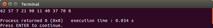
}From the preceding code, we create another function besides main(), that is, GenerateRandomNumber(). The code will invoke the function ten times using the for loop, as we can see in the preceding code. The output we will get should be as follows:
Back to the others loop statements which we discussed earlier, which are while and do...while loop. They are quite similar based on their behavior. The difference is when we use the while loop, there is a chance the statement inside the loop scope is not run, whereas the statement in the loop scope must be run at least once in the do...while loop.
Now, let's create a simple game using those loop statements. The computer will generate a number between 1 to 100, and then the user has to guess what number has been generated by the computer. The program will give a hint to the user just after she or he inputs the guessed number. It will tell the user whether the number is greater than the computer's number or lower than it. If the guessed number matches with the computer's number, the game is over. The code should be as follows:
// While.cbp
#include <iostream>
#include <cstdlib>
#include <ctime>
using namespace std;
int GenerateRandomNumber(int min, int max)
{
// static used for efficiency,
// so we only calculate this value once
static const double fraction =
1.0 / (static_cast<double>(RAND_MAX) + 1.0);
// evenly distribute the random number
// across our range
return min + static_cast<int>(
(max - min + 1) * (rand() * fraction));
}
int main()
{
// set initial seed value to system clock
srand(static_cast<unsigned int>(time(0)));
// Computer generate random number
// between 1 to 100
int computerNumber = GenerateRandomNumber(1, 100);
// User inputs a guessed number
int userNumber;
cout << "Please enter a number between 1 to 100: ";
cin >> userNumber;
// Run the WHILE loop
while(userNumber != computerNumber)
{
cout << userNumber << " is ";
if(userNumber > computerNumber)
cout << "greater";
else
cout << "lower";
cout << " than computer's number" << endl;
cout << "Choose another number: ";
cin >> userNumber;
}
cout << "Yeeaayy.. You've got the number." << endl;
return 0;
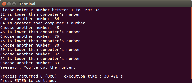
}From the preceding code, we can see that we have two variables, computerNumber and userNumber, handling the number that will be compared. There will be a probability that computerNumber is equal to userNumber. If this happens, the statement inside the while loop scope won't be executed at all. The flow of the preceding program can be seen in the following output console screenshot:
We have successfully implemented the while loop in the preceding code. Although the while loop is similar to the do...while loop, as we discussed earlier, we cannot refactor the preceding code by just replacing the while loop with the do...while loop. However, we can create another game as our example in implementing the do...while loop. However, now the user has to choose a number and then the program will guess it. The code should be as follows:
// Do-While.cbp
#include <iostream>
#include <cstdlib>
#include <ctime>

using namespace std;

int GenerateRandomNumber(int min, int max)
{
    // static used for efficiency,
    // so we only calculate this value once
    static const double fraction =
        1.0 / (static_cast<double>(RAND_MAX) + 1.0);

    // evenly distribute the random number
    // across our range
    return min + static_cast<int>(
        (max - min + 1) * (rand() * fraction));
}

int main()
{
    // set initial seed value to system clock
    srand(static_cast<unsigned int>(time(0)));

    char userChar;

    int iMin = 1;
    int iMax = 100;
    int iGuess;

    // Menu display
    cout << "Choose a number between 1 to 100, ";
    cout << "and I'll guess your number." << endl;
    cout << "Press L and ENTER if my guessed number is lower than
     yours";
    cout << endl;
    cout << "Press G and ENTER if my guessed number is greater than
     yours";
    cout << endl;
    cout << "Press Y and ENTER if I've successfully guessed your
     number!";
    cout << endl << endl;

    // Run the DO-WHILE loop
    do
    {
        iGuess = GenerateRandomNumber(iMin, iMax);
        cout << "I guess your number is " << iGuess << endl;
        cout << "What do you think? ";
        cin >> userChar;
        if(userChar == 'L' || userChar == 'l')
            iMin = iGuess + 1;
        else if(userChar == 'G' || userChar == 'g')
            iMax = iGuess - 1;

    }
    while(userChar != 'Y' && userChar != 'y');

    cout << "Yeeaayy.. I've got your number." << endl;
    return 0;
}
As we can see in the preceding code, the program has to guess the user's number at least once, and if it's lucky, the guessed number matches with the user's number, so that we use the do...while loop here. When we build and run the code, we will have an output similar to the following screenshot:
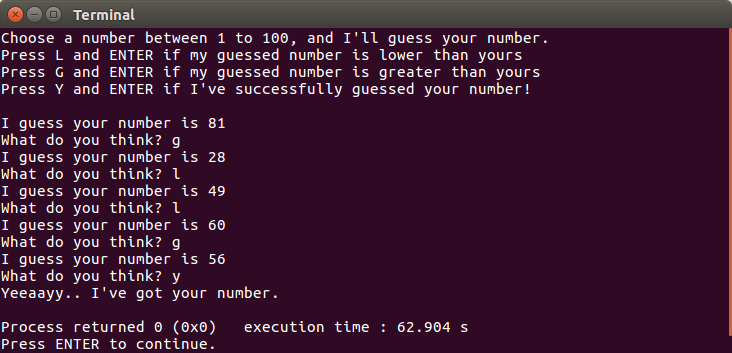
In the preceding screenshot, I chose number 56. The program then guessed 81. Since the number is greater than my number, the program guessed another number, which is 28. It then guessed another number based on the hint from me until it found the correct number. The program will leave the do...while loop if the user presses y, as we can see in the preceding code.
We have discussed the fundamental data type in the previous section. This data type is used in defining or initializing a variable to ensure that the variable can store the selected data type. However, there are other data types that can be used to define a variable. They are enum (enumeration) and struct.
Enumeration is a data type that has several possible values and they are defined as the constant which is called enumerators. It is used to create a collection of constants. Suppose we want to develop a card game using C++. As we know, a deck of playing cards contains 52 cards, which consists of four suits (Clubs, Diamonds, Hearts, and Spades) with 13 elements in each suit. We can notate the card deck as follows:
enum CardSuits
{
    Club,
    Diamond,
    Heart,
    Spade
};

enum CardElements
{
    Ace,
    Two,
    Three,
    Four,
    Five,
    Six,
    Seven,
    Eight,
    Nine,
    Ten,
    Jack,
    Queen,
    King
};
If we want to apply the preceding enum data types (CardSuits and CardElements), we can use the following variable initialization:
CardSuits suit = Club;
CardElements element = Ace;
Actually, enums always contain integer constants. The string we put in the enum element is the constant name only. The first element holds a value of 0, except we define another value explicitly. The next elements are in an incremental number from the first element. So, for our preceding CardSuits enum, Club is equal to 0, and the Diamond, Heart, and Spade are 1, 2, and 3, respectively.
Now, let's create a program that will generate a random card. We can borrow the GenerateRandomNumber() function from our previous code. The following is the complete code for this purpose:
// Enum.cbp
#include <iostream>
#include <cstdlib>
#include <ctime>

using namespace std;

enum CardSuits
{
    Club,
    Diamond,
    Heart,
    Spade
};

enum CardElements
{
    Ace,
    Two,
    Three,
    Four,
    Five,
    Six,
    Seven,
    Eight,
    Nine,
    Ten,
    Jack,
    Queen,
    King
};

string GetSuitString(CardSuits suit)
{
    string s;

    switch(suit)
    {
        case Club:
            s = "Club";
            break;
        case Diamond:
            s = "Diamond";
            break;
        case Heart:
            s = "Heart";
            break;
        case Spade:
            s = "Spade";
            break;
    }

    return s;
}

string GetElementString(CardElements element)
{
    string e;

    switch(element)
    {
        case Ace:
            e = "Ace";
            break;
        case Two:
            e = "Two";
            break;
        case Three:
            e = "Three";
            break;
        case Four:
            e = "Four";
            break;
        case Five:
            e = "Five";
            break;
        case Six:
            e = "Six";
            break;
        case Seven:
            e = "Seven";
            break;
        case Eight:
            e = "Eight";
            break;
        case Nine:
            e = "Nine";
            break;
        case Ten:
            e = "Ten";
            break;
        case Jack:
            e = "Jack";
            break;
        case Queen:
            e = "Queen";
            break;
        case King:
            e = "King";
            break;
    }

    return e;
}

int GenerateRandomNumber(int min, int max)
{
    // static used for efficiency,
    // so we only calculate this value once
    static const double fraction =
        1.0 / (static_cast<double>(RAND_MAX) + 1.0);

    // evenly distribute the random number
    // across our range
    return min + static_cast<int>(
        (max - min + 1) * (rand() * fraction));
}

int main()
{
    // set initial seed value to system clock
    srand(static_cast<unsigned int>(time(0)));

    // generate random suit and element card
    int iSuit = GenerateRandomNumber(0, 3);
    int iElement = GenerateRandomNumber(0, 12);

    CardSuits suit = static_cast<CardSuits>(
        iSuit);
    CardElements element = static_cast<CardElements>(
        iElement);

    cout << "Your card is ";
    cout << GetElementString(element);
    cout << " of " << GetSuitString(suit) << endl;

    return 0;
}
From the preceding code, we can see that we can access the enum data by using an integer value. However, we have to cast the int value so that it can fit the enum data by using static_cast<>, which is shown as follows:
int iSuit = GenerateRandomNumber(0, 3);
int iElement = GenerateRandomNumber(0, 12);

CardSuits suit = static_cast<CardSuits>(iSuit);
CardElements element = static_cast<CardElements>(iElement);
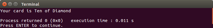
If we build and run the code, we will get the following console output:
Another advanced data type we have in C++ is structs. It is an aggregate data type which groups multiple individual variables together. From the preceding code, we have the suit and element variables that can be grouped as follows:
struct Cards
{
    CardSuits suit;
    CardElements element;
};
If we add the preceding struct to our preceding Enum.cbp code, we just need to refactor the main() function as follows:
int main()
{
    // set initial seed value to system clock
    srand(static_cast<unsigned int>(time(0)));

    Cards card;
    card.suit = static_cast<CardSuits>(
        GenerateRandomNumber(0, 3));
    card.element = static_cast<CardElements>(
        GenerateRandomNumber(0, 12));

    cout << "Your card is ";
    cout << GetElementString(card.element);
    cout << " of " << GetSuitString(card.suit) << endl;

    return 0;
}
If we run the preceding code (you can find the code as Struct.cbp in the repository), we will get the same output as Enum.cbp.
An abstract data type (ADT) is a type that consists of a collection of data and associated operations for manipulating the data. The ADT will only mention the list of operations that can be performed but not the implementation. The implementation itself is hidden, which is why it's called abstract.
Imagine we have a DVD player we usually use in our pleasure time. The player has a remote control, too. The remote control has various menu buttons such as ejecting the disc, playing or stopping the video, increasing or decreasing volume, and so forth. Similar to the ADT, we don't have any idea how the player increases the volume when we press the increasing button (similar to the operation in ADT). We just call the increasing operation and then the player does it for us; we do not need to know the implementation of that operation.
Regarding the process flow, we need to take into account the ADT's implement abstraction, information hiding, and encapsulation techniques. The explanation of these three techniques is as follows:
- Abstraction is hiding the implementation details of the operations that are available in the ADT
- Information hiding is hiding the data which is being affected by that implementation
- Encapsulation is grouping all similar data and functions into a group
Classes are containers for variables and the operations (methods) that will affect the variables. As we discussed earlier, as ADTs implement encapsulation techniques for grouping all similar data and functions into a group, the classes can also be applied to group them. A class has three access control sections for wrapping the data and methods, and they are:
- Public: Data and methods can be accessed by any user of the class
- Protected: Data and methods can only be accessed by class methods, derived classes, and friends
- Private: Data and methods can only be accessed by class methods and friends
Let's go back to the definition of abstraction and information hiding in the previous section. We can implement abstraction by using protected or private keywords to hide the methods from outside the class and implement the information hiding by using a protected or private keyword to hide the data from outside the class.
Now, let's build a simple class named Animal, as shown in the following code snippet:
class Animal
{
private:
    string m_name;

public:
    void GiveName(string name)
    {
        m_name = name;
    }

    string GetName()
    {
        return m_name;
    }
};
As we can see in the preceding code snippet, we cannot access the m_name variable directly since we assigned it as private. However, we have two public methods to access the variable from the inside class. The GiveName() methods will modify the m_name value, and the GetName() methods will return the m_name value. The following is the code to consume the Animal class:
// Simple_Class.cbp
#include <iostream>
using namespace std;
class Animal
{
private:
string m_name;
public:
void GiveName(string name)
{
m_name = name;
}
string GetName()
{
return m_name;
}
};
int main()
{
Animal dog = Animal();
dog.GiveName("dog");
cout << "Hi, I'm a " << dog.GetName() << endl;
return 0;
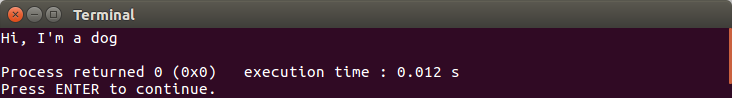
}In the preceding code, we created a variable named dog of the type Animal. Since then, the dog has the ability that Animal has, such as invoking the GiveName() and GetName() methods. The following is the window we should see if we build and run the code:
Now, we can say that Animal ADT has two functions, and they are GiveName(string name) and GetName().
After discussing simple class, you might see that there's a similarity between structs and classes. They both actually have similar behaviors. The differences are, however, that structs have the default public members, while classes have the default private members. I personally recommend using structs as data structures only (they don't have any methods in them) and using classes to build the ADTs.
As we can see in the preceding code, we assign the variable to the instance of the Animal class by using its constructor, which is shown as follows:
Animal dog = Animal();
However, we can initialize a class data member by using a class constructor. The constructor name is the same as the class name. Let's refactor our preceding Animal class so it has a constructor. The refactored code should be as follows:
// Constructor.cbp
#include <iostream>

using namespace std;

class Animal
{
private:
    string m_name;

public:
    Animal(string name) : m_name(name)
    {

    }

    string GetName()
    {
        return m_name;
    }
};

int main()
{
    Animal dog = Animal("dog");

    cout << "Hi, I'm a " << dog.GetName() << endl;

    return 0;
}
As we can see in the preceding code, when we define the dog variable, we also initialize the m_name private variable of the class. We don't need the GiveName() method anymore to assign the private variable. Indeed, we will get the same output again if we build and run the preceding code.
In the preceding code, we assign dog as the Animal data type. However, we can also derive a new class based on the base class. By deriving from the base class, the derived class will also have the behavior that the base class has. Let's refactor the Animal class again. We will add a virtual method named MakeSound(). The virtual method is a method that has no implementation yet, and only has the definition (also known as the interface). The derived class has to add the implementation to the virtual method using the override keyword, or else the compiler will complain. After we have a new Animal class, we will make a class named Dog that derives from the Animal class. The code should be as follows:
// Derived_Class.cbp
#include <iostream>
using namespace std;
class Animal
{
private:
string m_name;
public:
Animal(string name) : m_name(name)
{
}
// The interface that has to be implemented
// in derived class
virtual string MakeSound() = 0;
string GetName()
{
return m_name;
}
};
class Dog : public Animal
{
public:
// Forward the constructor arguments
Dog(string name) : Animal(name) {}
// here we implement the interface
string MakeSound() override
{
return "woof-woof!";
}
};
int main()
{
Dog dog = Dog("Bulldog");
cout << dog.GetName() << " is barking: ";
cout << dog.MakeSound() << endl;
return 0;
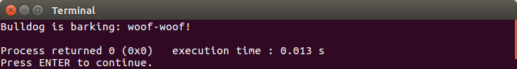
}Now, we have two classes, the Animal class (as the base class) and the Dog class (as the derived class). As shown in the preceding code, the Dog class has to implement the MakeSound() method since it has been defined as a virtual method in the Animal class. The instance of the Dog class can also invoke the GetName() method, even though it's not implemented inside the Dog class since the derived class derives all base class behavior. If we run the preceding code, we will see the following console window:
Again, we can say that the Dog ADT has two functions, and they are the GetName() and MakeSound() functions.
Another necessary requirement of ADT is that it has to be able to control all copy operations to avoid dynamic memory aliasing problems caused by shallow copying (some members of the copy may reference the same objects as the original). For this purpose, we can use assignment operator overloading. As the sample, we will refactor the Dog class so it now has the copy assignment operator. The code should be as follows:
// Assignment_Operator_Overload.cbp
#include <iostream>

using namespace std;

class Animal
{
protected:
    string m_name;

public:
    Animal(string name) : m_name(name)
    {

    }

    // The interface that has to be implemented
    // in derived class
    virtual string MakeSound() = 0;

    string GetName()
    {
        return m_name;
    }
};

class Dog : public Animal
{
public:
    // Forward the constructor arguments
    Dog(string name) : Animal(name) {}

    // Copy assignment operator overloading
    void operator = (const Dog &D)
    {
         m_name = D.m_name;
    }

    // here we implement the interface
    string MakeSound() override
    {
        return "woof-woof!";
    }
};

int main()
{
    Dog dog = Dog("Bulldog");
    cout << dog.GetName() << " is barking: ";
    cout << dog.MakeSound() << endl;

    Dog dog2 = dog;
    cout << dog2.GetName() << " is barking: ";
    cout << dog2.MakeSound() << endl;

    return 0;
}
We have added a copy assignment operator which is overloading in the Dog class. However, since we tried to access the m_name variable in the base class from the derived class, we need to make m_nameprotected instead of private. In the main() method, when we copy dog to dog2 in Dog dog2 = dog;, we can ensure that it's not a shallow copy.
Now, let's play with the templates. The templates are the features that allow the functions and classes to operate with generic types. It makes a function or class work on many different data types without having to be rewritten for each one. Using the template, we can build various data types, which we will discuss later in this book.
Suppose we have another class that is derived from the Animal class, for instance, Cat. We are going to make a function that will invoke the GetName() and MakeSound() methods for both the Dog and Cat instances. Without creating two separated functions, we can use the template, which is shown as follows:
// Function_Templates.cbp
#include <iostream>
using namespace std;
class Animal
{
protected:
string m_name;
public:
Animal(string name) : m_name(name)
{
}
// The interface that has to be implemented
// in derived class
virtual string MakeSound() = 0;
string GetName()
{
return m_name;
}
};
class Dog : public Animal
{
public:
// Forward the constructor arguments
Dog(string name) : Animal(name) {}
// Copy assignment operator overloading
void operator = (const Dog &D)
{
m_name = D.m_name;
}
// here we implement the interface
string MakeSound() override
{
return "woof-woof!";
}
};
class Cat : public Animal
{
public:
// Forward the constructor arguments
Cat(string name) : Animal(name) {}
// Copy assignment operator overloading
void operator = (const Cat &D)
{
m_name = D.m_name;
}
// here we implement the interface
string MakeSound() override
{
return "meow-meow!";
}
};
template<typename T>
void GetNameAndMakeSound(T& theAnimal)
{
cout << theAnimal.GetName() << " goes ";
cout << theAnimal.MakeSound() << endl;
}
int main()
{
Dog dog = Dog("Bulldog");
GetNameAndMakeSound(dog);
Cat cat = Cat("Persian Cat");
GetNameAndMakeSound(cat);
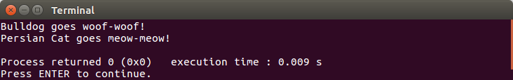
return 0;
}From the preceding code, we can see that we can pass both the Dog and Cat data types to the GetNameAndMakeSound() function since we have defined the <typename T> template before the function definition. The typename is a keyword in C++, which is used to write a template. The keyword is used for specifying that a symbol in a template definition or declaration is a type (in the preceding example, the symbol is T). As a result, the function becomes generic and can accept various data types, and if we build and run the preceding code, we will be shown the following console window:
Please ensure that the data type we pass to the generic function has the ability to do all the operation invoking from the generic function. However, the compiler will compile if the data type we pass does not have the expected operation. In the preceding function template example, we need to pass a data type that is an instance of the Animal class, so we can pass either instance of the Animal class or an instance of a derived class of the Animal class.
Similar to the function template, the class template is used to build a generic class that can accept various data types. Let's refactor the preceding Function_Template.cbp code by adding a new class template. The code should be as follows:
// Class_Templates.cbp
#include <iostream>

using namespace std;

class Animal
{
protected:
    string m_name;

public:
    Animal(string name) : m_name(name)
    {

    }

    // The interface that has to be implemented
    // in derived class
    virtual string MakeSound() = 0;

    string GetName()
    {
        return m_name;
    }
};

class Dog : public Animal
{
public:
    // Forward the constructor arguments
    Dog(string name) : Animal(name) {}

    // Copy assignment operator overloading
    void operator = (const Dog &D)
    {
         m_name = D.m_name;
    }

    // here we implement the interface
    string MakeSound() override
    {
        return "woof-woof!";
    }
};

class Cat : public Animal
{
public:
    // Forward the constructor arguments
    Cat(string name) : Animal(name) {}

    // Copy assignment operator overloading
    void operator = (const Cat &D)
    {
         m_name = D.m_name;
    }

    // here we implement the interface
    string MakeSound() override
    {
        return "meow-meow!";
    }

};

template<typename T>
void GetNameAndMakeSound(T& theAnimal)
{
    cout << theAnimal.GetName() << " goes ";
    cout << theAnimal.MakeSound() << endl;
}

template <typename T>
class AnimalTemplate
{
private:
    T m_animal;

public:
    AnimalTemplate(T animal) : m_animal(animal) {}

    void GetNameAndMakeSound()
    {
        cout << m_animal.GetName() << " goes ";
        cout << m_animal.MakeSound() << endl;
    }
};

int main()
{
    Dog dog = Dog("Bulldog");
    AnimalTemplate<Dog> dogTemplate(dog);
    dogTemplate.GetNameAndMakeSound();

    Cat cat = Cat("Persian Cat");
    AnimalTemplate<Cat> catTemplate(cat);
    catTemplate.GetNameAndMakeSound();

    return 0;
}
As we can see in the preceding code, we have a new class named AnimalTemplate. It's a template class and it can be used by any data type. However, we have to define the data type in the angle bracket, as we can see in the preceding code, when we use the instances dogTemplate and catTemplate. If we build and run the code, we will get the same output as we did for the Function_Template.cbp code.
C++ programming has another powerful feature regarding the use of template classes, which is the Standard Template Library. It's a set of class templates to provide all functions that are commonly used in manipulating various data structures. There are four components that build the STL, and they are algorithms, containers, iterators, and functions. Now, let's look at these components further.
Algorithms are used on ranges of elements, such as sorting and searching. The sorting algorithm is used to arrange the elements, both in ascending and descending order. The searching algorithm is used to look for a specific value from the ranges of elements.
Containers are used to store objects and data. The common container that is widely used is vector. The vector is similar to an array, except it has the ability to resize itself automatically when an element is inserted or deleted.
Iterators are used to work upon a sequence of values. Each container has its own iterator. For instance, there are begin(), end(), rbegin(), and rend() functions in the vector container.
Functions are used to overload the existing function. The instance of this component is called a functor, or function object. The functor is defined as a pointer of a function where we can parameterize the existing function.
We are not building any code in this section since we just need to know that the STL is a powerful library in C++ and that it exists, fortunately. We are going to discuss the STL deeper in the following chapters while we construct data structures.
To create a good algorithm, we have to ensure that we have got the best performance from the algorithm. In this section, we are going to discuss the ways we can analyze the time complexity of basic functions.
Let's start with asymptotic analysis to find out the time complexity of the algorithms. This analysis omits the constants and the least significant parts. Suppose we have a function that will print a number from 0 to n. The following is the code for the function:
void Looping(int n)
{
    int i = 0;

    while(i < n)
    {
        cout << i << endl;
        i = i + 1;
    }
}
Now, let's calculate the time complexity of the preceding algorithm by counting each instruction of the function. We start with the first statement:
int i = 0;
The preceding statement is only executed once in the function, so its value is 1. The following is the code snippet of the rest statements in the Looping() function:
while(i < n)
{
    cout << i << endl;
    i = i + 1;
}
The comparison in the while loop is valued at 1. For simplicity, we can say that the value of the two statements inside the while loop scope is 3 since it needs 1 to print the i variable, and 2 for assignment (=) and addition (+).
However, how much of the preceding code snippet is executed depends on the value of n, so it will be (1 + 3) * n or 4n. The total instruction that has to be executed for the preceding Looping() function is 1 + 4n. Therefore, the complexity of the preceding Looping() function is:
Time Complexity(n) = 4n + 1
And here is the curve that represents its complexity:
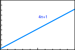
In all curve graphs that will be represented in this book, the x axis represents Input Size (n) and the y axis represents Execution Time.
As we can see in the preceding graph, the curve is linear. However, since the time complexity also depends on the other parameters, such as hardware specification, we may have another complexity for the preceding Looping() function if we run the function on faster hardware. Let's say the time complexity becomes 2n + 0.5, so that the curve will be as follow:
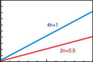
As we can see, the curve is still linear for the two complexities. For this reason, we can omit a constant and the least significant parts in asymptotic analysis, so we can say that the preceding complexity is n, as found in the following notation:
Time Complexity(n) = n
Let's move on to another function. If we have the nested while loop, we will have another complexity, as we can see in the following code:
void Pairing(int n)
{
int i = 0;
while(i < n)
{
int j = 0;
while(j < n)
{
cout << i << ", " << j << endl;
j = j + 1;
}
i = i + 1;
}
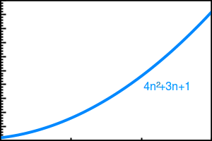
}Based on the preceding Looping() function, we can say that the complexity of the inner while loop of the preceding Pairing() function is 4n + 1. We then calculate the outer while loop so it becomes 1 + (n * (1 + (4n + 1) + 2), which equals 1 + 3n + 4n2. Therefore, the complexity of the preceding code is:
Time Complexity(n) = 4n2 + 3n + 1
The curve for the preceding complexity will be as follows:
And if we run the preceding code in the slower hardware, the complexity might become twice as slow. The notation should be as follows:
Time Complexity(n) = 8n2 + 6n + 2
And the curve of the preceding notation should be as follows:
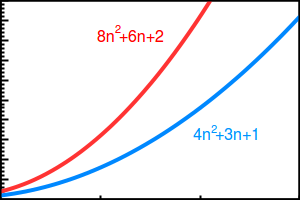
As shown previously, since the asymptotic analysis omits the constants and the least significant parts, the complexity notation will be as follows:
Time Complexity(n) = n2
In the previous section, we were able to define time complexity for our code using an asymptotic algorithm. In this section, we are going to determine a case of the implementation of an algorithm. There are three cases when implementing time complexity in an algorithm; they are worst, average, and best cases. Before we go through them, let's look at the following Search() function implementation:
int Search(int arr[], int arrSize, int x)
{
    // Iterate through arr elements
    for (int i = 0; i < arrSize; ++i)
    {
        // If x is found
        // returns index of x
        if (arr[i] == x)
            return i;
    }

    // If x is not found
    // returns -1
    return -1;
}
As we can see in the preceding Search() function, it will find an index of target element (x) from an arr array containing arrSize elements. Suppose we have the array {42, 55, 39, 71, 20, 18, 6, 84}. Here are the cases we will find:
- Worst case analysis is a calculation of the upper bound on the running time of the algorithm. In the
Search()function, the upper bound can be an element that does not appear in thearr, for instance,60, so it has to iterate through all elements ofarrand still cannot find the element. - Average case analysis is a calculation of all possible inputs on the running time of algorithm, including an element that is not present in the
arrarray. - Best case analysis is a calculation of the lower bound on the running time of the algorithm. In the
Search()function, the lower bound is the first element of thearrarray, which is42. When we search for element42, the function will only iterate through thearrarray once, so thearrSizedoesn't matter.
After discussing asymptotic analysis and the three cases in algorithms, let's discuss asymptotic notation to represent the time complexity of an algorithm. There are three asymptotic notations that are mostly used in an algorithm; they are Big Theta, Big-O, and Big Omega.
The Big Theta notation (θ) is a notation that bounds a function from above and below, like we saw previously in asymptotic analysis, which also omits a constant from a notation.
Suppose we have a function with time complexity 4n + 1. Since it's a linear function, we can notate it like in the following code:
f(n) = 4n + 1
Now, suppose we have a function, g(n), where f(n) is the Big-Theta of g(n) if the value, f(n), is always between c1*g(n) (lower bound) and c2*g(n) (upper bound). Since f(n) has a constant of 4 in the n variable, we will take a random lower bound which is lower than 4, that is 3, and an upper bound which is greater than 4, that is 5. Please see the following curve for reference:
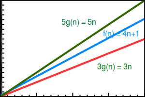
From the f(n) time complexity, we can get the asymptotic complexity n, so then we have g(n) = n, which is based on the asymptotic complexity of 4n + 1. Now, we can decide the upper bound and lower bound for g(n) = n. Let's pick 3 for the lower bound and 5 for the upper bound. Now, we can manipulate the g(n) = n function as follows:
3.g(n) = 3.n
5.g(n) = 5.n
Big-O notation (O) is a notation that bounds a function from above only using the upper bound of an algorithm. From the previous notation, f(n) = 4n + 1, we can say that the time complexity of the f(n) is O(n). If we are going to use Big Theta notation, we can say that the worst case time complexity of f(n) is θ(n) and the best case time complexity of f(n) is θ(1).
Big Omega notation is contrary to Big-O notation. It uses the lower bound to analyze time complexity. In other words, it uses the best case in Big Theta notation. For the f(n) notation, we can say that the time complexity is Ω(1).
In the previous code sample, we calculated the complexity of the iterative method. Now, let's do this with the recursive method. Suppose we need to calculate the factorial of a certain number, for instance 6, which will produce 6 * 5 * 4 * 3 * 2 * 1 = 720. For this purpose, we can use the recursive method, which is shown in the following code snippet:
int Factorial(int n)
{
    if(n == 1)
        return 1;

    return n * Factorial(n - 1);
}
For the preceding function, we can calculate the complexity similarly to how we did for the iterative method, which is f(n) = n since it depends on how much data is being processed (which is n). We can use a constant, for instance c, to calculate the lower bound and the upper bound.
In the previous section, we just discussed the single input, n, for calculating the complexity. However, sometimes we will deal with more than just one input. Please look at the following SumOfDivision() function implementation:
int SumOfDivision(
    int nArr[], int n, int mArr[], int m)
{
    int total = 0;

    for(int i = 0; i < n; ++i)
    {
        for(int j = 0; j < m; ++j)
        {
            total += (nArr[i] * mArr[j]);
        }
    }

    return total;
}
And that's where amortized analysis comes in. Amortized analysis calculates the complexity of performing the operation for varying inputs, for instance, when we insert some elements into several arrays. Now, the complexity doesn't only depend on the n input only, but also the m input. The complexity can be as follows:
Time Complexity(n, m) = n · m
We are going to discuss these analysis methods in more detail in the following chapters.
This chapter provided us with an introduction to basic C++ (simple program, IDE, flow control) and all data types (fundamental and advanced data types, including template and STL) that we will use to construct the data structures in the following chapters. We also discussed a basic complexity analysis, and we will dig into this deeper in the upcoming chapters.
Next, we are going to create our first data structures, that is, linked list, and we are going to perform some operations on the data structure.
- What is the first function in C++ which is executed for the first time?
- Please list the fundamental data types in C++!
- What can we use to control the flow of code?
- What is the difference between enums and structs?
- What are the abstraction, information hiding, and encapsulation techniques? Please explain!
- What is the keyword to create a template in C++?
- What is the difference between the function template and the class template?
- What is the difference between Big Theta, Big-O, and Big Omega?
You can also refer to the following links: