In this chapter, we will learn about the core concepts of Bayesian statistics and some of the instruments in the Bayesian toolbox. We will use some Python code, but this chapter will be mostly theoretical; most of the concepts we will see here will be revisited many times throughout this book. This chapter, being heavy on the theoretical side, may be a little anxiogenic for the coder in you, but I think it will ease the path in effectively applying Bayesian statistics to your problems.

In this chapter, we will cover the following topics:

• Statistical modeling
• Probabilities and uncertainty
• Bayes' theorem and statistical inference
• Single-parameter inference and the classic coin-flip problem
• Choosing priors and why people often don't like them, but should
• Communicating a Bayesian analysis

Statistics is about collecting, organizing, analyzing, and interpreting data, and hence statistical knowledge is essential for data analysis. Two main statistical methods are used in data analysis:

• Exploratory Data Analysis (EDA): This is about numerical summaries, such as the mean, mode, standard deviation, and interquartile ranges (this part of EDA is also known as descriptive statistics). EDA is also about visually inspecting the data, using tools you may be already familiar with, such as histograms and scatter plots.
• Inferential statistics: This is about making statements beyond the current data. We may want to understand some particular phenomenon, or maybe we want to make predictions for future (as yet unobserved) data points, or we need to choose among several competing explanations for the same observations. Inferential statistics is the set of methods and tools that will help us to answer these types of questions.

Most introductory statistical courses, at least for non-statisticians, are taught as a collection of recipes that more or less go like this: go to the statistical pantry, pick one tin can and open it, add data to taste, and stir until you obtain a consistent p-value, preferably under 0.05. The main goal in this type of course is to teach you how to pick the proper can. I never liked this approach, mainly because the most common result is a bunch of confused people unable to grasp, even at the conceptual level, the unity of the different learned methods. We will take a different approach: we will also learn some recipes, but this will be homemade rather than canned food; we will learn how to mix fresh ingredients that will suit different gastronomic occasions and, more importantly, that will let you to apply concepts far beyond the examples in this book.

Taking this approach is possible for two reasons:

• Ontological: Statistics is a form of modeling unified under the mathematical framework of probability theory. Using a probabilistic approach provides a unified view of what may seem like very disparate methods; statistical methods and machine learning (ML) methods look much more similar under the probabilistic lens.
• Technical: Modern software, such as PyMC3, allows practitioners, just like you and me, to define and solve models in a relative easy way. Many of these models were unsolvable just a few years ago or required a high level of mathematical and technical sophistication.

Data is an essential ingredient in statistics and data science. Data comes from several sources, such as experiments, computer simulations, surveys, and field observations. If we are the ones in charge of generating or gathering the data, it is always a good idea to first think carefully about the questions we want to answer and which methods we will use, and only then proceed to get the data. In fact, there is a whole branch of statistics dealing with data collection, known as experimental design. In the era of the data deluge, we can sometimes forget that gathering data is not always cheap. For example, while it is true that the Large Hadron Collider (LHC) produces hundreds of terabytes a day, its construction took years of manual and intellectual labor.

As a general rule, we can think of the process generating the data as stochastic, because there is ontological, technical, and/or epistemic uncertainty, that is, the system is intrinsically stochastic, there are technical issues adding noise or restricting us from measuring with arbitrary precision, and/or there are conceptual limitations veiling details from us. For all these reasons, we always need to interpret data in the context of models, including mental and formal ones. Data does not speak but through models.

In this book, we will assume that we already have collected the data. Our data will also be clean and tidy, something rarely true in the real world. We will make these assumptions in order to focus on the subject of this book. I just want to emphasize, especially for newcomers to data analysis, that even when not covered in this book, these are important skills that you should learn and practice in order to successfully work with data.

A very useful skill when analyzing data is knowing how to write code in a programming language, such as Python. Manipulating data is usually necessary given that we live in a messy world with even messier data, and coding helps to get things done. Even if you are lucky and your data is very clean and tidy, coding will still be very useful since modern Bayesian statistics is done mostly through programming languages such as Python or R.

If you want to learn how to use Python for cleaning and manipulating data, I recommend reading the excellent book, Python Data Science Handbook, by Jake VanderPlas.

Models are simplified descriptions of a given system or process that, for some reason, we are interested in. Those descriptions are deliberately designed to capture only the most relevant aspects of the system and not to explain every minor detail. This is one reason a more complex model is not always a better one.

There are many different kinds of models; in this book, we will restrict ourselves to Bayesian models. We can summarize the Bayesian modeling process using three steps:

1. Given some data and some assumptions on how this data could have been generated, we design a model by combining building blocks known as probability distributions. Most of the time these models are crude approximations, but most of the time is all we need.
2. We use Bayes' theorem to add data to our models and derive the logical consequences of combining the data and our assumptions. We say we are conditioning the model on our data.
3. We criticize the model by checking whether the model makes sense according to different criteria, including the data, our expertise on the subject, and sometimes by comparing several models.

In general, we will find ourselves performing these three steps in an iterative non-linear fashion. We will retrace our steps at any given point: maybe we made a silly coding mistake, or we found a way to change the model and improve it, or we realized that we need to add more data or collect a different kind of data.

Bayesian models are also known as probabilistic models because they are built using probabilities. Why probabilities? Because probabilities are the correct mathematical tool to model uncertainty, so let's take a walk through the garden of forking paths.

The title of this section may be a little bit pretentious as we are not going to learn probability theory in just a few pages, but that is not my intention. I just want to introduce a few general and important concepts that are necessary to better understand Bayesian methods, and that should be enough for understanding the rest of the book. If necessary, we will expand or introduce new probability-related concepts as we need them. For a detailed study of probability theory, I highly recommend the book, Introduction to Probability by Joseph K Blitzstein and Jessica Hwang. Another useful book could be Mathematical Theory of Bayesian Statistics by Sumio Watanabe, as the title says, the book is more Bayesian-oriented than the first, and also heavier on the mathematical side.

While probability theory is a mature and well-established branch of mathematics, there is more than one interpretation of probability. From a Bayesian perspective, a probability is a measure that quantifies the uncertainty level of a statement. Under this definition of probability, it is totally valid and natural to ask about the probability of life on Mars, the probability of the mass of the electron being 9.1 x 10^-31 kg, or the probability of the 9^th of July of 1816 being a sunny day in Buenos Aires. Notice, for example, that life on Mars exists or does not exist; the outcome is binary, a yes-no question. But given that we are not sure about that fact, a sensible course of action is trying to find out how likely life on Mars is. Since this definition of probability is related to our epistemic state of mind, people often call it the subjective definition of probability. But notice that any scientific-minded person will not use their personal beliefs, or the information provided by an angel to answer such a question, instead they will use all the relevant geophysical data about Mars, and all the relevant biochemical knowledge about necessary conditions for life, and so on. Therefore, Bayesian probabilities, and by extension Bayesian statistics, is as subjective (or objective) as any other well-established scientific method we have.

If we do not have information about a problem, it is reasonable to state that every possible event is equally likely, formally this is equivalent to assigning the same probability to every possible event. In the absence of information, our uncertainty is maximum. If we know instead that some events are more likely, then this can be formally represented by assigning higher probability to those events and less to the others. Notice than when we talk about events in stats-speak, we are not restricting ourselves to things that can happen, such as an asteroid crashing into Earth or my auntie's 60^th birthday party; an event is just any of the possible values (or subset of values) a variable can take, such as the event that you are older than 30, or the price of a Sachertorte, or the number of bikes sold last year around the world.

The concept of probability it is also related to the subject of logic. Under Aristotelian or classical logic, we can only have statements that take the values of true or false. Under the Bayesian definition of probability, certainty is just a special case: a true statement has a probability of 1, a false statement has probability of 0. We would assign a probability of 1 to the statement, There is Martian life, only after having conclusive data indicating something is growing, and reproducing, and doing other activities we associate with living organisms. Notice, however, that assigning a probability of 0 is harder because we can always think that there is some Martian spot that is unexplored, or that we have made mistakes with some experiment, or several other reasons that could lead us to falsely believe life is absent on Mars even when it is not. Related to this point is Cromwell's rule, stating that we should reserve the use of the prior probabilities of 0 or 1 to logically true or false statements. Interestingly enough, Richard Cox mathematically proved that if we want to extend logic to include uncertainty, we must use probabilities and probability theory. Bayes' theorem is just a logical consequence of the rules of probability, as we will see soon. Hence, another way of thinking about Bayesian statistics is as an extension of logic when dealing with uncertainty, something that clearly has nothing to do with subjective reasoning in the pejorative sense—people often used the term subjective.

To summarize, using probability to model uncertainty is not necessarily related to the debate about whether nature is deterministic or random at is most fundamental level, nor is related to subjective personal beliefs. Instead, it is a purely methodological approach to model uncertainty. We recognize most phenomena are difficult to grasp because we generally have to deal with incomplete and/or noisy data, we are intrinsically limited by our evolution-sculpted primate brain, or any other sound reason you could add. As a consequence, we use a modeling approach that explicitly takes uncertainty into account.

Now that we've discussed the Bayesian interpretation of probability, let's learn about a few of the mathematical properties of probabilities.

Probabilities are numbers in the [0, 1] interval, that is, numbers between 0 and 1, including both extremes. Probabilities follow a few rules; one of these rules is the product rule:

We read this as follows: the probability of and is equal to the probability of given , times the probability of . The expression represents the joint probability of and . The expression is used to indicate a conditional probability; the name refers to the fact that the probability of is conditioned on knowing . For example, the probability that the pavement is wet is different from the probability that the pavement is wet if we know (or given that) it's raining. A conditional probability can be larger than, smaller than, or equal to the unconditioned probability. If knowing does not provides us with information about , then . This will be true only if and are independent of each other. On the contrary, if knowing gives us useful information about , then the conditional probability could be larger or smaller than the unconditional probability, depending on whether knowing makes less or more likely. Let's see a simple example using a fair six-sided die. What is the probability of getting the number 3 if we roll the die, ? This is 1/6 since each of the six numbers has the same chance for a fair six-sided die. And what is the probability of getting the number 3 given that we have obtained an odd number, ? This is 1/3, because if we know we have an odd number, the only possible numbers are and each of them has the same chance. Finally, what is the probability of ? This is 0, because if we know the number is even, then the only possible ones are , and thus getting a 3 is not possible.

As we can see from this simple example, by conditioning on observed data we effectively change the probability of events, and with it, the uncertainty we have about them. Conditional probabilities are the heart of statistics, irrespective of your problem being rolling dice or building self-driving cars.

A probability distribution is a mathematical object that describes how likely different events are. In general, these events are restricted somehow to a set of possible events, such as for a die (we exclude undefined). A common and useful conceptualization in statistics is to think data is generated from some true probability distribution with unknown parameters. Then, inference is the process of finding out the values of those parameters using just a sample (also known as a dataset) from the true probability distribution. In general, we do not have access to the true probability distribution and thus we must resign ourselves and create a model in an attempt to somehow approximate that distribution. Probabilistic models are built by properly combining probability distributions.

If a variable, , can be described by a probability distribution, then we call a random variable. As a general rule, people use capital letters, such as , to indicate the objects random variable, and , to indicate an instance of that random variable. can be a vector and thus contains many elements or individual values . Let's see an example using Python; our true probability distribution will be a Normal (or Gaussian) distribution with means of and ; these two parameters completely and unambiguously define a Normal distribution. Using SciPy, we can define the random variable, , by writing stats.norm(μ, σ) and we can get an instance, , from it using the rvs (random variates) method. In the following example, we ask for three values:

μ = 0.
σ = 1.
X = stats.norm(μ, σ)
x = X.rvs(3)

You will notice that each time you execute this code (in stats-speak: every trial), you will get a different random result. Notice that once the values of the parameters of a distributions are known, the probability of each value is also known; what is random is the exact values we will get at each trial. A common misconception with the meaning of random is that you can get any possible value from a random variable or that all values are equally likely. The allowed values of a random variable and their probabilities are strictly controlled by a probability distribution, and the randomness arises only from the fact that we can not predict the exact values we will get in each trial. Every time we execute the preceding code, we will get three different numbers, but if we iterate the code thousands of times, we will be able to empirically check that the mean of the sampled values is around zero and that 95% of the samples will have values within the [-1.96, +1.96] range. Please do not trust me, use your Pythonic powers and verify it for yourself. We can arrive at this same conclusion if we study the mathematical properties of the Normal distribution.

A common notation used in statistics to indicate that a variable is distributed as a normal distribution with parameters and is:

In this context, when you find the (tilde) symbol, say is distributed as.

In many texts, it is common to see the normal distribution expressed in terms of the variance and not the standard deviation. Thus, people write . In this book, we are going to parameterize the Normal distribution using the standard deviation, first because it is easier to interpret, and second because this is how PyMC3 works.

We will meet several probability distributions in this book; every time we discover one, we will take a moment to describe it. We started with the normal distribution because it is like the Zeus of the probability distributions. A variable, , follows a Gaussian distribution if its values are dictated by the following expression:

This is the probability density function for the Normal distribution; you do not need to memorize expression 1.3, I just like to show it to you so you can see where the numbers come from. As we have already mentioned, and are the parameters of the distribution, and by specifying those values we totally define the distribution; you can see this from expression 1.3 as the other terms are all constants. can take any real value, that is, , and dictates the mean of the distribution (and also the median and mode, which are all equal). is the standard deviation, which can only be positive and dictates the spread of the distribution, the larger the value of , the more spread out the distribution. Since there are an infinite number of possible combinations of and , there is an infinite number of instances of the Gaussian distribution and all of them belong to the same Gaussian family.

Mathematical formulas are concise and unambiguous and some people say even beautiful, but we must admit that meeting them for the first time can be intimidating, specially for those not very mathematically inclined; a good way to break the ice is to use Python to explore them:

mu_params = [-1, 0, 1]
sd_params = [0.5, 1, 1.5]
x = np.linspace(-7, 7, 200)
_, ax = plt.subplots(len(mu_params), len(sd_params), sharex=True, 
                     sharey=True,
                     figsize=(9, 7), constrained_layout=True)
for i in range(3):
    for j in range(3):
        mu = mu_params[i]
        sd = sd_params[j]
        y = stats.norm(mu, sd).pdf(x)
        ax[i,j].plot(x, y)
        ax[i,j].plot([], label="μ = {:3.2f}\nσ = {:3.2f}".format(mu, 
                     sd), alpha=0)
        ax[i,j].legend(loc=1)
ax[2,1].set_xlabel('x')
ax[1,0].set_ylabel('p(x)', rotation=0, labelpad=20)
ax[1,0].set_yticks([])

Most of the preceding code is for plotting, the probabilistic part is performed by the y = stats.norm(mu, sd).pdf(x) line. With this line, we are evaluating the probability density function of the normal distribution, given the mu and sd parameters for a set of x values. The preceding code generates Figure 1.1. In each subplot we have a blue (dark gray) curve representing a Gaussian distribution with specific parameters, and , included in each subplot's legend:

There are two types of random variables: continuous and discrete. Continuous variables can take any value from some interval (we can use Python floats to represent them), and discrete variables can take only certain values (we can use Python integers to represent them). The Normal distribution is a continuous distribution.

Notice that in the preceding plot, the yticks are omitted; this is a feature not a bug. The reason to omit them is that, in my experience, those values do not add too much relevant information and could be potentially confusing to some people. Let me explain myself: the actual numbers on the y axis do not really matter—what is relevant is their relative values. If you take two values from , let's say and _, and you find that (two times higher in the plot), you can safely say the probability of the value of is twice the probability of . This is something that most people will understand intuitively, and fortunately is the correct interpretation. The only tricky part when dealing with continuous distributions is that the values plotted on the y axis are not probabilities, but probability densities. To get a proper probability, you have to integrate between a given interval, that is, you have to compute the area below the curve (for that interval). While probabilities cannot be greater than one, probability densities can, and is the total area under the probability density curve the one restricted to be 1. Understanding the difference between probabilities and probability densities is crucial from a mathematical point of view. For the practical approach used in this book, we can be a little bit more sloppy, since that difference is not that important as long as you get the correct intuition on how to interpret the previous plot in terms of relative values.

Many models assume that successive values of random variables are all sampled from the same distribution and those values are independent of each other. In such a case, we will say that the variables are independently and identically distributed (iid) variables for short. Using mathematical notation, we can see that two variables are independent if for every value of and .

A common example of non-iid variables are temporal series, where a temporal dependency in the random variable is a key feature that should be taken into account. Take, for example, the following data coming from http://cdiac.esd.ornl.gov. This data is a record of atmospheric CO₂ measurements from 1959 to 1997. We are going to load the data (including the accompanying code) and plot it:

data = np.genfromtxt('../data/mauna_loa_CO2.csv', delimiter=',')
plt.plot(data[:,0], data[:,1])
plt.xlabel('year')
plt.ylabel('$CO_2$ (ppmv)')
plt.savefig('B11197_01_02.png', dpi=300)

Each data point corresponds to the measured levels of atmospheric CO₂ per month. The temporal dependency of data points is easy to see in this plot. In fact, we have two trends here: a seasonal one (this is related to cycles of vegetation growth and decay), and a global one, indicating an increasing concentration of atmospheric CO₂.

Now that we have learned some of the basic concepts and jargon from probability theory, we can move to the moment everyone was waiting for. Without further ado, let's contemplate, in all its majesty, Bayes' theorem:

Well, it's not that impressive, is it? It looks like an elementary school formula, and yet, paraphrasing Richard Feynman, this is all you need to know about Bayesian statistics.

Learning where Bayes' theorem comes from will help us to understand its meaning.

According to the product rule we have:

This can also be written as:

Given that the terms on the left are equal for equations 1.5 and 1.6, we can combine them and write:

And if we reorder 1.7, we get expression 1.4, thus is Bayes' theorem.

Now, let's see what formula 1.4 implies and why it is important. First, it says that is not necessarily the same as . This is a very important fact, one that is easy to miss in daily situations even for people trained in statistics and probability. Let's use a simple example to clarify why these quantities are not necessarily the same. The probability of a person being the Pope given that this person is Argentinian is not the same as the probability of being Argentinian given that this person is the Pope. As there are around 44,000,000 Argentinians alive and a single one of them is the current Pope, we have and we also have _.

If we replace with hypothesis and with data, Bayes' theorem tells us how to compute the probability of a hypothesis, , given the data, , and that's the way you will find Bayes' theorem explained in a lot of places. But, how do we turn a hypothesis into something that we can put inside Bayes' theorem? Well, we do it by using probability distributions. So, in general, our hypothesis is a hypothesis in a very, very, very narrow sense; we will be more precise if we talk about finding a suitable value for parameters in our models, that is, parameters of probability distributions. By the way, don't try to set to statements such as unicorns are real, unless you are willing to build a realistic probabilistic model of unicorn existence!

Bayes' theorem is central to Bayesian statistics, as we will see in Chapter 2, Programming Probabilistically using tool such as PyMC3 free ourselves of the need to explicitly write Bayes' theorem every time we build a Bayesian model. Nevertheless, it is important to know the name of its parts because we will constantly refer to them and it is important to understand what each part means because this will help us to conceptualize models, so let's do it:

• : Prior
• : Likelihood
• : Posterior
• : Marginal likelihood

The prior distribution should reflect what we know about the value of the parameter before seeing the data, . If we know nothing, like Jon Snow, we could use flat priors that do not convey too much information. In general, we can do better than flat priors, as we will learn in this book. The use of priors is why some people still talk about Bayesian statistics as subjective, even when priors are just another assumption that we made when modeling and hence are just as subjective (or objective) as any other assumption, such as likelihoods.

The likelihood is how we will introduce data in our analysis. It is an expression of the plausibility of the data given the parameters. In some texts, you will find people call this term sampling model, statistical model, or just model. We will stick to the name likelihood and we will call the combination of priors and likelihood model.

The posterior distribution is the result of the Bayesian analysis and reflects all that we know about a problem (given our data and model). The posterior is a probability distribution for the parameters in our model and not a single value. This distribution is a balance between the prior and the likelihood. There is a well-known joke: A Bayesian is one who, vaguely expecting a horse, and catching a glimpse of a donkey, strongly believes he has seen a mule. One excellent way to kill the mood after hearing this joke is to explain that if the likelihood and priors are both vague, you will get a posterior reflecting vague beliefs about seeing a mule rather than strong ones. Anyway, I like the joke, and I like how it captures the idea of a posterior being somehow a compromise between prior and likelihood. Conceptually, we can think of the posterior as the updated prior in the light of (new) data. In fact, the posterior from one analysis can be used as the prior for a new analysis. This makes Bayesian analysis particularly suitable for analyzing data that becomes available in sequential order. Some examples could be an early warning system for natural disasters that processes online data coming from meteorological stations and satellites. For more details, read about online machine learning methods.

The last term is the marginal likelihood, also known as evidence. Formally, the marginal likelihood is the probability of observing the data averaged over all the possible values the parameters can take (as prescribed by the prior). Anyway, for most of this book, we will not care about the marginal likelihood, and we will think of it as a simple normalization factor. We can do this because when analyzing the posterior distribution, we will only care about the relative values of the parameters and not their absolute values. You may remember that we mentioned this when we talked about how to interpret plots of probability distributions in the previous section. If we ignore the marginal likelihood, we can write Bayes' theorem as a proportionality:

Understanding the exact role of each term in Bayes' theorem will take some time and practice, and it will require we work through a few examples, and that's what the rest of this book is for.

In the last two sections, we learned several important concepts, but two of them are essentially the core of Bayesian statistics, so let's restate them in a single sentence.

Now that we know what Bayesian statistics is, let's learn how to do Bayesian statistics with a simple example. We are going to begin inferring a single, unknown parameter.

The coin-flipping problem, or the beta-binomial model if you want to sound fancy at parties, is a classical problem in statistics and goes like this: we toss a coin a number of times and record how many heads and tails we get. Based on this data, we try to answer questions such as, is the coin fair? Or, more generally, how biased is the coin? While this problem may sound dull, we should not underestimate it. The coin-flipping problem is a great example to learn the basics of Bayesian statistics because it is a simple model that we can solve and compute with ease. Besides, many real problems consist of binary, mutually-exclusive outcomes such as 0 or 1, positive or negative, odds or evens, spam or ham, hotdog or not hotdog, cat or dog, safe or unsafe, and healthy or unhealthy. Thus, even when we are talking about coins, this model applies to any of those problems.

In order to estimate the bias of a coin, and in general to answer any questions in a Bayesian setting, we will need data and a probabilistic model. For this example, we will assume that we have already tossed a coin a number of times and we have a record of the number of observed heads, so the data-gathering part is already done. Getting the model will take a little bit more effort. Since this is our first model, we will explicitly write Bayes' theorem and do all the necessary math (don't be afraid, I promise it will be painless) and we will proceed very slowly. From Chapter 2, Programming Probabilistically, onward, we will use PyMC3 and our computer to do the math for us.

The first thing we will do is generalize the concept of bias. We will say that a coin with a bias of 1 will always land heads, one with a bias of 0 will always land tails, and one with a bias of 0.5 will land half of the time heads and half of the time tails. To represent the bias, we will use the parameter, and to represent the total number of heads for a number of tosses, we will use the variable. According to Bayes' theorem (equation 1.4), we have to specify the prior, , and likelihood, , we will use. Let's start with the likelihood.

Let's assume that only two outcomes are possible—heads or tails—and let's also assume that a coin toss does not affect other tosses, that is, we are assuming coin tosses are independent of each other. We will further assume all coin tosses come from the same distribution. Thus the random variable coin toss is an example of an iid variable. I hope you agree these are very reasonable assumptions to make for our problem. Given these assumptions a good candidate for the likelihood is the binomial distribution:

This is a discrete distribution returning the probability of getting heads (or in general, successes) out of coin tosses (or in general, trials or experiments) given a fixed value of :

n_params = [1, 2, 4]  # Number of trials
p_params = [0.25, 0.5, 0.75]  # Probability of success

x = np.arange(0, max(n_params)+1)
f,ax = plt.subplots(len(n_params), len(p_params), sharex=True, 
                    sharey=True,
                    figsize=(8, 7), constrained_layout=True)

for i in range(len(n_params)):
    for j in range(len(p_params)):
        n = n_params[i]
        p = p_params[j]

        y = stats.binom(n=n, p=p).pmf(x)

        ax[i,j].vlines(x, 0, y, colors='C0', lw=5)
        ax[i,j].set_ylim(0, 1)
        ax[i,j].plot(0, 0, label="N = {:3.2f}\nθ = 
                           {:3.2f}".format(n,p), alpha=0)
        ax[i,j].legend()

        ax[2,1].set_xlabel('y')
        ax[1,0].set_ylabel('p(y | θ, N)')
        ax[0,0].set_xticks(x)

The preceding figure shows nine binomial distributions; each subplot has its own legend indicating the values of the parameters. Notice that for this plot I did not omit the values on the y axis. I did this so you can check for yourself that if you sum the high of all bars you will get 1, that is, for discrete distributions, the height of the bars represents actual probabilities.

The binomial distribution is a reasonable choice for the likelihood. We can see that indicates how likely it is to obtain a head when tossing a coin (this is easier to see when , but is valid for any value of )—just compare the value of with the height of the bar for (heads).

OK, if we know the value of , the binomial distribution will tell us the expected distribution of heads. The only problem is that we do not know ! But do not despair; in Bayesian statistics, every time we do not know the value of a parameter, we put a prior on it, so let's move on and choose a prior for .

As a prior, we will use a beta distribution, which is a very common distribution in Bayesian statistics and looks as follows:

If we look carefully, we will see that the beta distribution looks similar to the binomial except for the first term, the one with all those . The first term is a normalizing constant that ensures the distribution integrates to 1, and is the Greek uppercase gamma letter and represents what is known as gamma function. We can see from the preceding formula that the beta distribution has two parameters, and . Using the following code, we will explore our third distribution so far:

params = [0.5, 1, 2, 3]
x = np.linspace(0, 1, 100)
f, ax = plt.subplots(len(params), len(params), sharex=True, 
                     sharey=True,
                     figsize=(8, 7), constrained_layout=True)
for i in range(4):
    for j in range(4):
        a = params[i]
        b = params[j]
        y = stats.beta(a, b).pdf(x)
        ax[i,j].plot(x, y)
        ax[i,j].plot(0, 0, label="α = {:2.1f}\nβ = {:2.1f}".format(a, 
                     b), alpha=0)
        ax[i,j].legend()
ax[1,0].set_yticks([])
ax[1,0].set_xticks([0, 0.5, 1])
f.text(0.5, 0.05, 'θ', ha='center')
f.text(0.07, 0.5, 'p(θ)', va='center', rotation=0)

I really like the beta distribution and all the shapes we can get from it, but why are we using it for our model? There are many reasons to use a beta distribution for this and other problems. One of them is that the beta distribution is restricted to be between 0 and 1, in the same way our parameter is. In general, we use the beta distribution when we want to model proportions of a binomial variable. Another reason is for its versatility. As we can see in the preceding figure, the distribution adopts several shapes (all restricted to the [0, 1] interval), including a uniform distribution, Gaussian-like distributions, and U-like distributions. As a third reason, the beta distribution is the conjugate prior of the binomial distribution (which we are using as the likelihood). A conjugate prior of a likelihood is a prior that, when used in combination with a given likelihood, returns a posterior with the same functional form as the prior. Untwisting the tongue, every time we use a beta distribution as the prior and a binomial distribution as the likelihood, we will get a beta as the posterior distribution. There are other pairs of conjugate priors; for example, the Normal distribution is the conjugate prior of itself. For many years, Bayesian analysis was restricted to the use of conjugate priors. Conjugacy ensures mathematical tractability of the posterior, which is important given that a common problem in Bayesian statistics is ending up with a posterior we cannot solve analytically. This was a deal breaker before the development of suitable computational methods to solve probabilistic methods. From Chapter 2, Programming Probabilistically onwards, we will learn how to use modern computational methods to solve Bayesian problems, whether we choose conjugate priors or not.

Let's remember that Bayes' theorem (equation 1.4) says the posterior is proportional to the likelihood times the prior. So, for our problem, we have to multiply the binomial and the beta distributions:

We can simplify this expression. For our practical concerns, we can drop all the terms that do not depend on and our results will still be valid. Accordingly, we can write:

Reordering it, we get:

If we pay attention, we will see that this expression has the same functional form of a beta distribution (except for the normalization term) with and . In fact, the posterior distribution for our problem is the beta distribution:

Now we will use Python to compute and plot the posterior distribution based on the analytical expression we have just derived. In the following code, you will see there is actually one line that computes the results while the others are there just to get a nice plot:

plt.figure(figsize=(10, 8))

n_trials = [0, 1, 2, 3, 4, 8, 16, 32, 50, 150]
data = [0, 1, 1, 1, 1, 4, 6, 9, 13, 48]
theta_real = 0.35

beta_params = [(1, 1), (20, 20), (1, 4)]
dist = stats.beta
x = np.linspace(0, 1, 200)

for idx, N in enumerate(n_trials):
    if idx == 0:
        plt.subplot(4, 3, 2)
        plt.xlabel('θ')
    else:
        plt.subplot(4, 3, idx+3)
        plt.xticks([])
    y = data[idx]
    for (a_prior, b_prior) in beta_params:
        p_theta_given_y = dist.pdf(x, a_prior + y, b_prior + N - y)
        plt.fill_between(x, 0, p_theta_given_y, alpha=0.7)

    plt.axvline(theta_real, ymax=0.3, color='k')
    plt.plot(0, 0, label=f'{N:4d} trials\n{y:4d} heads', alpha=0)
    plt.xlim(0, 1)
    plt.ylim(0, 12)
    plt.legend()
    plt.yticks([])
plt.tight_layout()

On the first subplot of Figure 1.5, we have zero trials, thus the three curves represent our priors:

• The uniform (blue) prior. This represent all the possible values for the bias being equally probable a priori.
• The Gaussian-like (orange) prior is centered and concentrated around 0.5, so this prior is compatible with information indicating that the coin has more or less about the same chance of landing heads or tails. We could also say this prior is compatible with the belief that most coins are fair. While belief is commonly used in Bayesian discussions, we think is better to talk about models and parameters that are informed by data.
• The skewed (green) prior puts the most weight on a tail-biased outcome.

The rest of the subplots show posterior distributions for successive trials. The number of trials (or coin tosses) and the number of heads are indicated in each subplot's legend. There is also a black vertical line at 0.35 representing the true value for . Of course, in real problems, we do not know this value, and it is here just for pedagogical reasons. This figure can teach us a lot about Bayesian analysis, so grab your coffee, tea, or favorite drink and let's take a moment to understand it:

• The result of a Bayesian analysis is a posterior distribution, not a single value but a distribution of plausible values given the data and our model.
• The most probable value is given by the mode of the posterior (the peak of the distribution).
• The spread of the posterior is proportional to the uncertainty about the value of a parameter; the more spread out the distribution, the less certain we are.
• Intuitively, we are more confident in a result when we have observed more data supporting that result. Thus, even when numerically , seeing four heads out of eight trials gives us more confidence that the bias is 0.5 than observing one head out of two trials. This intuition is reflected in the posterior, as you can check for yourself if you pay attention to the (blue) posterior in the third and sixth subplots; while the mode is the same, the spread (uncertainty) is larger in the third subplot than in the sixth subplot.
• Given a sufficiently large amount of data, two or more Bayesian models with different priors will tend to converge to the same result. In the limit of infinite data, no matter which prior we use, all of them will provide the same posterior. Remember that infinite is a limit and not a number, so from a practical point of view, we could get practically indistinguishably posteriors for a finite and rather small number of data points.
• How fast posteriors converge to the same distribution depends on the data and the model. In the preceding figure, we can see that the posteriors coming from the blue prior (uniform) and green prior (biased towards tails) converge faster to almost the same distribution, while it takes longer for the orange posterior (the one coming from the concentrated prior). In fact, even after 150 trials, it is somehow easy to recognize the orange posterior as a different distribution from the two others.
• Something not obvious from the figure is that we will get the same result if we update the posterior sequentially than if we do it all at once. We can compute the posterior 150 times, each time adding one more observation and using the obtained posterior as the new prior, or we can just compute one posterior for the 150 tosses at once. The result will be exactly the same. This feature not only makes perfect sense, it also leads to a natural way of updating our estimations when we get new data, a situation common in many data-analysis problems.

From the preceding example, it is clear that priors can influence inferences. This is totally fine, priors are supposed to do this. Newcomers to Bayesian analysis (as well as detractors of this paradigm) are generally a little nervous about how to choose priors, because they do not want the prior to act as a censor that does not let the data speak for itself! That's OK, but we have to remember that data does not really speak; at best, data murmurs. Data only makes sense in the context of our models, including mathematical and mental models. There are plenty of examples in the history of science where the same data leads people to think differently about the same topics, and this can happen even if you base your opinions on formal models.

Some people like the idea of using non-informative priors (also known as flat, vague, or diffuse priors); these priors have the least possible amount of impact on the analysis. While it is possible to use them, in general, we can do better. Throughout this book, we will follow the recommendations of Gelman, McElreath, Kruschke, and many others, and we will prefer weakly-informative priors. For many problems, we often know something about the values a parameter can take, we may know that a parameter is restricted to being positive, or we may know the approximate range it can take, or whether we expect the value to be close to zero or below/above some value. In such cases, we can use priors to put some weak information in our models without being afraid of being too pushy. Because these priors work to keep the posterior distribution within certain reasonable bounds, they are also known as regularizing priors. Using informative priors is also a valid option if we have good-quality information to define those priors. Informative priors are very strong priors that convey a lot of information. Depending on your problem, it could be easy or not to find this type of prior. For example, in my field of work (structural bioinformatics), people have been using, in Bayesian and non-Bayesian ways, all the prior information they could get to study and especially predict the structure of proteins. This is reasonable because we have been collecting data from thousands of carefully-designed experiments for decades and hence we have a great amount of trustworthy prior information at our disposal. Not using it would be absurd! So, the take-home message is this: if you have reliable prior information, there is no reason to discard that information, including the nonsensical argument that being objective means throwing away valuable information. Imagine if every time an automotive engineer had to design a new car, they had to start from scratch and reinvent the combustion engine, the wheel, and for that matter, the whole concept of a car. That's not the way things should work.

Knowing we can classify priors into categories according to their relative strength does not make us less nervous about choosing from them. Maybe it would be better to not have priors at all—that would make modeling easier, right? Well, not necessarily. Priors can make models behave better, have better generalization properties, and can help us convey useful information. Also, every model, Bayesian or not, has some kind of prior in one way or another, even if the prior is not set explicitly. In fact, many result from frequentist statistics, and can be seen as special cases of a Bayesian model under certain circumstances, such as flat priors. One common frequentist method to estimate parameters is known as maximum likelihood; this methods avoids setting a prior and works just by finding the value of that maximizes the likelihood. This value is usually notated by adding a little hat on top of the symbol of the parameter we are estimating, such as or sometimes (or even both). is a point estimate (a number) and not a distribution. For the coin-flipping problem we can compute this analytically:

If you go back to Figure 1.5, you will be able to check for yourself that the mode of the blue posterior (the one corresponding to the uniform/flat prior) agrees with the values of , computed for each subplot. So, at least for this example, we can see that even when the maximum likelihood method does not explicitly invoke any prior, it can be considered a special case of a Bayesian model, one with a uniform prior.

We cannot really avoid priors, but if we include them in our analysis, we will get several benefits, including a distribution of plausible values and not only the most probable one. Another advantage of being explicit about priors is that we get more transparent models, meaning they're easier to criticize, debug (in a broad sense of the word), and hopefully improve. Building models is an iterative process; sometimes the iteration takes a few minutes, sometimes it could take years. Sometimes it will only involve you, and sometimes it will involve people you do not even know. Reproducibility matters and transparent assumptions in a model contribute to it. Besides, we are free to use more than one prior (or likelihood) for a given analysis if we are not sure about any special one; exploring the effect of different priors can also bring valuable information to the table. Part of the modeling process is about questioning assumptions, and priors (and likelihood) are just that. Different assumptions will lead to different models and probably different results. By using data and our domain knowledge of the problem, we will be able to compare models and, if necessary, decide on a winner. Chapter 5, Model Comparison, will be devoted to this issue. Since priors have a central role in Bayesian statistics, we will keep discussing them as we face new problems. So if you have doubts and feel a little bit confused about this discussion, just keep calm and don't worry, people have been confused for decades and the discussion is still going on.

Creating reports and communicating results is central to the practice of statistics and data science. In this section, we will briefly discuss some of the peculiarities of this task when working with Bayesian models. In future chapters, we will keep looking at examples about this important matter.

If you want to communicate the results of an analysis, you should also communicate the model you used. A common notation to succinctly represent probabilistic models is:

This is just the model we use for the coin-flip example. As you may remember, the symbol indicates that the variable, on the left of it, is a random variable distributed according to the distribution on the right. In many contexts, this symbol is used to indicate that a variable takes approximately some value, but when talking about probabilistic models, we will read this symbol out loud saying is distributed as. Thus, we can say is distributed as a beta distribution with and parameters, and is distributed as a binomial with and parameters. The very same model can be represented graphically using Kruschke's diagrams:

On the first level, we have the prior that generates the values for , then the likelihood, and on the last line the data, . Arrows indicate the relationship between variables, and the symbol indicates the stochastic nature of the variables. All Kruschke's diagrams in the book were made using the templates provided by Rasmus Bååth (http://www.sumsar.net/blog/2013/10/diy-kruschke-style-diagrams/).

The result of a Bayesian analysis is a posterior distribution, and all the information about the parameters given a dataset and a model is contained in the posterior distribution. Thus, by summarizing the posterior, we are summarizing the logical consequences of a model and data. A common practice is to report, for each parameter, the mean (or mode or median) to have an idea of the location of the distribution and some measure, such as the standard deviation, to have an idea of the dispersion and hence the uncertainty in our estimate. The standard deviation works well for normal-like distributions but can be misleading for other type of distributions, such as skewed ones. So, an alternative is to use the following measure.

A commonly-used device to summarize the spread of a posterior distribution is to use a Highest-Posterior Density (HPD) interval. An HPD is the shortest interval containing a given portion of the probability density. One of the most commonly-used is the 95% HPD, often accompanied by the 50% HPD. If we say that the 95% HPD for some analysis is [2-5], we mean that according to our data and model, we think the parameter in question is between 2 and 5 with a probability of 0.95.

ArviZ is a Python package for exploratory data analysis for Bayesian models. ArviZ has many functions to help us summarize the posterior, for example, az.plot_posterior can be used to generate a plot with the mean and HPD of a distribution. In the following example, instead of a posterior from a real analysis, we are generating a random sample from a beta distribution:

np.random.seed(1)
az.plot_posterior({'θ':stats.beta.rvs(5, 11, size=1000)})

Note that in Figure 1.7, the reported HPD is 94%. This is a friendly remainder of the arbitrary nature of the 95% value. Every time ArviZ computes and reports a HPD, it will use, by default, a value of 0.94 (corresponding to 94%). You can change this by passing a different value to the credible_interval argument.

One of the nice elements of the Bayesian toolkit is that once we have a posterior, it is possible to use the posterior, , to generate predictions, , based on the data, , and the estimated parameters, . The posterior predictive distribution is:

Thus, the posterior predictive distribution is an average of conditional predictions over the posterior distribution of . Conceptually (and computationally), we approximate this integral 1.17 as an iterative two-step process:

1. We sample a value of from the posterior,
2. We feed that value of to the likelihood (or sampling distribution if you wish), thus obtaining a data point,

The generated predictions, , can be used when we need to make, ahem, predictions. But also we can use them to criticize the models by comparing the observed data, , and the predicted data, , to spot differences between these two sets, this is known as posterior predictive checks. The main goal is to check for auto-consistency. The generated data and the observed data should look more or less similar, otherwise there was some problem during the modeling or some problem feeding the data to the model. But even in the absence of mistakes, differences could arise. Trying to understand the mismatch could lead us to improve models or at least to understand their limitations. Knowing which parts of our problem/data the model is capturing well and which it is not is valuable information even if we do not know how to improve the model. Maybe the model captures the mean behavior of our data well but fails to predict rare values. This could be problematic for us, or maybe we only care about the mean, so this model will be OK to us. The general aim is not to declare that a model is false. We just want to know which part of the model we can trust, and try to test whether the model is a good fit for our specific purpose. How confident one can be about a model is certainly not the same across disciplines. Physics can study systems under highly-controlled conditions using high-level theories, so models are often seen as good descriptions of reality. Other disciplines, such as sociology and biology, study complex, difficult-to-isolate systems, and thus models usually have a weaker epistemological status. Nevertheless, independent of which discipline you are working in, models should always be checked, and posterior predictive checks together with ideas from exploratory data analysis are a good way to check our models.

We began our Bayesian journey with a very brief discussion about statistical modeling, probability theory, and the introduction of Bayes' theorem. We then used the coin-flipping problem as an excuse to introduce basic aspects of Bayesian modeling and data analysis. We used this classic example to convey some of the most important ideas of Bayesian statistics, such as using probability distributions to build models and represent uncertainties. We tried to demystify the use of priors and put them on an equal footing with other elements that are part of the modeling process, such as the likelihood, or even more meta-questions, such as why we are trying to solve a particular problem in the first place. We ended the chapter by discussing the interpretation and communication of the results of a Bayesian analysis.

Figure 1.8 is based on one from Sumio Watanabe and summarizes the Bayesian workflow as described in this chapter:

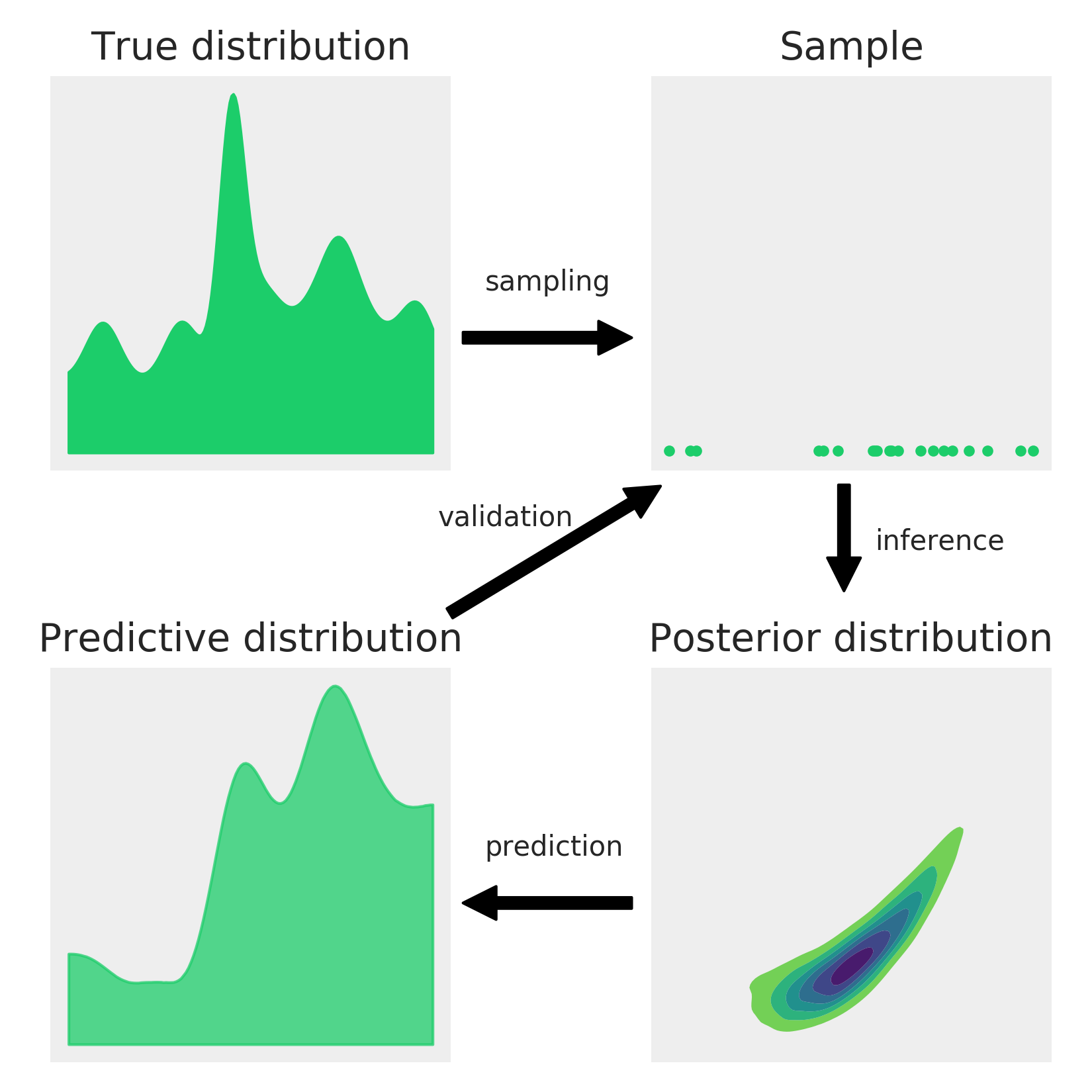
We assume there is a True distribution that in general is unknown (and in principle also unknowable), from which we get a finite sample, either by doing an experiment, a survey, an observation, or a simulation. In order to learn something from the True distribution, given that we have only observed a sample, we build a probabilistic model. A probabilistic model has two basic ingredients: a prior and a likelihood. Using the model and the sample, we perform Bayesian Inference and obtain a Posterior distribution; this distribution encapsulates all the information about a problem, given our model and data. From a Bayesian perspective, the posterior distribution is the main object of interest and everything else is derived from it, including predictions in the form of a Posterior Predictive Distribution. As the Posterior distribution (and any other derived quantity from it) is a consequence of the model and data, the usefulness of Bayesian inferences are restricted by the quality of models and data. One way to evaluate our model is by comparing the Posterior Predictive Distribution with the finite sample we got in the first place. Notice that the Posterior distribution is a distribution of the parameters in a model (conditioned on the observed samples), while the Posterior Predictive Distribution is a distribution of the predicted samples (averaged over the posterior distribution). The process of model validation is of crucial importance not because we want to be sure we have the right model, but because we know we almost never have the right model. We check models to evaluate whether they are useful enough in a specific context and, if not, to gain insight into how to improve them.

In this chapter, we have briefly summarized the main aspects of doing Bayesian data analysis. Throughout the rest of this book, we will revisit these ideas to really absorb them and use them as the scaffold of more advanced concepts. In the next chapter, we will introduce PyMC3, which is a Python library for Bayesian modeling and Probabilistic Machine Learning, and ArviZ, which is a Python library for the exploratory analysis of Bayesian models.

We do not know whether the brain really works in a Bayesian way, in an approximate Bayesian fashion, or maybe some evolutionary (more or less) optimized heuristics. Nevertheless, we know that we learn by exposing ourselves to data, examples, and exercises... well you may say that humans never learn, given our record as a species on subjects such as wars or economic systems that prioritize profit and not people's well-being... Anyway, I recommend you do the proposed exercises at the end of each chapter:

1. From the following expressions, which one corresponds to the sentence, The probability of being sunny given that it is 9^th of July of 1816?
   • p(sunny)
   • p(sunny | July)
   • p(sunny | 9^th of July of 1816)
   • p(9^th of July of 1816 | sunny)
   • p(sunny, 9^th of July of 1816) / p(9^th of July of 1816)
2. Show that the probability of choosing a human at random and picking the Pope is not the same as the probability of the Pope being human. In the animated series Futurama, the (Space) Pope is a reptile. How does this change your previous calculations?
3. In the following definition of a probabilistic model, identify the prior and the likelihood:
4. In the previous model, how many parameters will the posterior have? Compare it with the model for the coin-flipping problem.
5. Write the Bayes' theorem for the model in exercise 3.
6. Let's suppose that we have two coins; when we toss the first coin, half of the time it lands tails and half of the time on heads. The other coin is a loaded coin that always lands on heads. If we take one of the coins at random and get a head, what is the probability that this coin is the unfair one?
7. Modify the code that generated Figure 1.5 in order to add a dotted vertical line showing the observed rate head/(number of tosses), compare the location of this line to the mode of the posteriors in each subplot.
8. Try re-plotting Figure 1.5 using other priors (beta_params) and other data (trials and data).

9. Explore different parameters for the Gaussian, binomial, and beta plots (Figure 1.1, Figure 1.3, and Figure 1.4, respectively). Alternatively, you may want to plot a single distribution instead of a grid of distributions.
10. Read about the Cromwel rule on Wikipedia: https://en.wikipedia.org/wiki/Cromwell%27s_rule.
11. Read about probabilities and the Dutch book on Wikipedia: https://en.wikipedia.org/wiki/Dutch_book.