This book is for readers who have already begun a journey learning about robotics and wish to progress to a more advanced level of capability by adding AI behaviors to your robot, unmanned vehicle, or self-driving car. You may have already made a robot for yourself out of standard parts, and have a robot that can drive around, perhaps make a map, and avoid obstacles with some basic sensors. The question then is: what comes next?

The basic difference between what we will call an AI robot and a more normal robot is the ability of the robot and its software to make decisions, and learn and adapt to its environment based on data from its sensors. To be a bit more specific, we are leaving the world of deterministic behaviors behind. When we call a system deterministic, we mean that for a set of inputs, the robot will always produce the same output. If faced with the same situation, such as encountering an obstacle, then the robot will always do the same thing, such as go around the obstacle to the left. An AI robot, however, can do two things the standard robot cannot: make decisions and learn from experience. The AI robot will change and adapt to circumstances, and may do something different each time a situation is encountered. It may try to push the obstacle out of the way, or make up a new route, or change goals.

The following topics will be covered in this chapter:

• What is Artificial Intelligence (AI)?
• Modern AI – nothing new
• Our example problem
• What you will learn in this book – AI techniques covered
• Introduction to TinMan, our robot
• Keeping control – soft real-time control
• The OODA loop – basis for decision making

• Python 2.7 or 3.5 with numpy, scipy, matplotlib, and scikit-learn installed.
• Robotics Operating System (ROS) Kinetic Kame.
• A computer running Linux for development or a virtual machine running Linux under Windows. Ubuntu 16.04 is used for the examples and illustrations.
• Raspberry Pi 3 or a similar single board computer (BeagleBone Black, Odroid, or similar). We are not using the GPIO or special interfaces on the Pi3.
• An Arduino Mega 2560 microcontroller.

The repository for the source code in this chapter on GitHub is: https://github.com/FGovers/AI_and_Robotics_source_code/chapter_1

Check out the following video to see the Code in Action:
http://bit.ly/2BT0Met

Artificial intelligence applied to robotics development requires a different set of skills from you, the robot designer or developer. You may have made robots before. You probably have a quadcopter or a 3D printer (which is, in fact, a robot). The familiar world of Proportional Integral Derivative (PID) controllers, sensor loops, and state machines must give way to artificial neural networks, expert systems, genetic algorithms, and searching path planners. We want a robot that does not just react to its environment as a reflex action, but has goals and intent—and can learn and adapt to the environment. We want to solve problems that would be intractable or impossible otherwise.

What we are going to do in this book is introduce a problem – picking up toys in a playroom—that we will use as our example throughout the book as we learn a series of techniques for applying AI techniques to our robot. It is important to understand that in this book, the journey is far more important than the destination. At the end of the book, you should gain some important skills with broad applicability, not just learn how to pick up toys.

One of the difficult decisions I had to make about writing this book was deciding if this is an AI book about robotics or a robotics approach to AI—that is, is the focus learning about robotics or learning about AI? The answer is that this is a book about how to apply AI tools to robotics problems, and thus is primarily an AI book using robotics as an example. The tools and techniques learned will have applicability even if you don’t do robotics, but just apply AI to decision making to trade on the stock market.

What we are going to do is first provide some tools and background to match the infrastructure that was used to develop the examples in the book. This is both to provide an even playing field and to not assume any knowledge on the reader’s part. We will use the Python programming language, the ROS for our data infrastructure, and be running under the Linux operating system. I developed the examples in the book with Oracle’s VirtualBox software running Ubuntu Linux in a virtual machine on a Windows Vista computer. Our robot hardware will be a Raspberry Pi 3 as the robot’s on-board brain, and an Arduino Mega2560 as the hardware interface microcontroller.

In the rest of this chapter, we will discuss some basics about AI, and then proceed to develop two important tools that we will use in all of the examples in the rest of the book. We will introduce the concept of soft real-time control, and then provide a framework, or model, for interfacing AI to our robot called the Observe-Orient-Decide-Act (OODA) loop.

What would be a definition of AI? In general, it means a machine that exhibits some characteristics of intelligence—thinking, reasoning, planning, learning, and adapting. It can also mean a software program that can simulate thinking or reasoning. Let’s try some examples: a robot that avoids obstacles by simple rules (if the obstacle is to the right, go left) is not an AI. A program that learns by example to recognize a cat in a video, is an AI. A mechanical arm that is operated by a joystick is not AI, but a robot arm that adapts to different objects in order to pick them up is AI.

There are two defining characteristics of artificial intelligence robots that you must be aware of. First of all, AI robots learn and adapt to their environments, which means that they change behaviors over time. The second characteristic is emergent behavior, where the robot exhibits developing actions that we did not program into it explicitly. We are giving the robot controlling software that is inherently non-linear and self-organizing. The robot may suddenly exhibit some bizarre or unusual reaction to an event or situation that seems to be odd, or quirky, or even emotional. I worked with a self-driving car that we swore had delicate sensibilities and moved very daintily, earning it the nickname Ferdinand after the sensitive, flower loving bull from the cartoon, which was appropriate in a nine-ton truck that appeared to like plants. These behaviors are just caused by interactions of the various software components and control algorithms, and do not represent anything more than that.

One concept you will hear around AI circles is the Turing test. The Turing test was proposed by Alan Turing in 1950, in a paper entitled Computing Machinery and Intelligence. He postulated that a human interrogator would question an hidden, unseen AI system, along with another human. If the human posing the questions was unable to tell which person was the computer and which the human was, then that AI computer would pass the test. This test supposes that the AI would be fully capable of listening to a conversation, understanding the content, and giving the same sort of answers a person will. I don’t believe that AI has progressed to this point yet, but chat bots and automated answering services have done a good job of making you believe that you are talking to a human and not a robot.

Our objective in this book is not to pass the Turing test, but rather to take some novel approaches to solving problems using techniques in machine learning, planning, goal seeking, pattern recognition, grouping, and clustering. Many of these problems would be very difficult to solve any other way. A software AI that could pass the Turing test would be an example of a general artificial intelligence, or a full, working intelligent artificial brain, and just like you, a general AI does not need to be specifically trained to solve any particular problem. To date, a general AI has not been created, but what we do have is narrow AI, or software that simulates thinking in a very narrow application, such as recognizing objects, or picking good stocks to buy.

What we are not building in this book is a general AI, and we are not going to be worried about our creations developing a mind of their own or getting out of control. That comes from the realm of science fiction and bad movies, rather than the reality of computers today. I am firmly of the mind that anyone preaching about the evils of AI or predicting that robots will take over the world has not worked or practiced in this area, and has not seen the dismal state of AI research in respect of solving general problems or creating anything resembling an actual intelligence.

Most of AI as practiced today is not new. Most of these techniques were developed in the 1960s and 1970s and fell out of favor because the computing machinery of the day was insufficient for the complexity of the software or number of calculations required, and only waited for computers to get bigger, and for another very significant event – the invention of the internet. In previous decades, if you needed 10,000 digitized pictures of cats to compile a database to train a neural network, the task would be almost impossible—you could take a lot of cat pictures, or scan images from books. Today, a Google search for cat pictures returns 126,000,000 results in 0.44 seconds. Finding cat pictures, or anything else, is just a search away, and you have your training set for your neural network—unless you need to train on a very specific set of objects that don't happen to be on the internet, as we will see in this book, in which case we will once again be taking a lot of pictures with another modern aid not found in the 1960s, a digital camera. The happy combination of very fast computers; cheap, plentiful storage; and access to almost unlimited data of every sort has produced a renaissance in AI.

Another modern development has occurred on the other end of the computer spectrum. While anyone can now have a supercomputer on their desk at home, the development of the smartphone has driven a whole series of innovations that are just being felt in technology. Your wonder of a smartphone has accelerometers and gyroscopes made of tiny silicon chips called microelectromechanical systems (MEMS). It also has a high resolution but very small digital camera, and a multi-core computer processor that takes very little power to run. It also contains (probably) three radios: a WiFi wireless network, a cellular phone, and a Bluetooth transceiver. As good as these parts are at making your iPhone™ fun to use, they have also found their way into parts available for robots. That is fun for us because what used to be only available for research labs and universities are now for sale to individual users. If you happen to have a university or research lab, or work for a technology company with multi-million dollar development budgets, you will also learn something from this book, and find tools and ideas that hopefully will inspire your robotics creations or power new products with exciting capabilities.

In the course of this book, we will be using a single problem set that I feel most people can relate to easily, while still representing a real challenge for the most seasoned roboticist. We will be using AI and robotics techniques to pick up toys in my upstairs game room after my grandchildren have visited. That sound you just heard was the gasp from the professional robotics engineers and researchers in the audience. Why is this a tough problem, and why is it ideal for this book?

This problem is a close analog to the problem Amazon has in picking items off of shelves and putting them in a box to send to you. For the last several years, Amazon has sponsored the Amazon Robotics Challenge where they invited teams to try and pick items off shelves and put them into a box for cash prizes. They thought the program difficult enough to invite teams from around the world. The contest was won in 2017 by a team from Australia.

Let’s discuss the problem and break it down a bit. Later, in Chapter 2, we will do a full task analysis, use cases, and storyboards to develop our approach, but we can start here with some general observations.

Robotics designers first start with the environment – where does the robot work? We divide environments into two categories: structured and unstructured. A structured environment, such as the playing field for a first robotics competition, an assembly line, or lab bench, has everything in an organized space. You have heard the saying A place for everything and everything in its place—that is a structured environment. Another way to think about it, is that we know in advance where everything is or is going to be. We know what color things are, where they are placed in space, and what shape they are. A name for this type of information is a prior knowledge – things we know in advance. Having advanced knowledge of the environment in robotics is sometimes absolutely essential. Assembly line robots are expecting parts to arrive in exactly the position and orientation to be grasped and placed into position. In other words, we have arranged the world to suit the robot.

In the world of our game room, this is simply not an option. If I could get my grandchildren to put their toys in exactly the same spot each time, then we would not need a robot for this task. We have a set of objects that is fairly fixed – we only have so many toys for them to play with. We occasionally add things or lose toys, or something falls down the stairs, but the toys are a elements of a set of fixed objects. What they are not is positioned or oriented in any particular manner – they are just where they were left when the kids finished playing with them and went home. We also have a fixed set of furniture, but some parts move – the footstool or chairs can be moved around. This is an unstructured environment, where the robot and the software have to adapt, not the toys or furniture.

The problem is to have the robot drive around the room, and pick up toys. Let's break this task down into a series of steps:

1. We want the user to interact with the robot by talking to it. We want the robot to understand what we want it to do, which is to say, what our intent is for the commands we are giving it.
2. Once commanded to start, the robot will have to identify an object as being a toy, and not a wall, a piece of furniture, or a door.
3. The robot must avoid hazards, the most important being the stairs going down to the first floor. Robots have a particular problem with negative obstacles (dropoffs, curbs, cliffs, stairs, and so on), and that is exactly what we have here.
4. Once the robot finds a toy, it has to determine how to pick the toy up with its robot arm. Can it grasp the object directly, or must it scoop the item up, or push it along? We expect that the robot will try different ways to pick up toys and may need several trial and error attempts.
5. Once the toy is acquired by the robot arm, the robot needs to carry the toy to a toy box. The robot must recognize the toy box in the room, remember where it is for repeat trips, and then position itself to place the toy in the box. Again, more than one attempt may be required.
6. After the toy is dropped off, the robot returns to patrolling the room looking for more toys. At some point, hopefully, all of the toys are retrieved. It may have to ask us, the human, if the room is acceptable, or if it needs to continue cleaning.

What will we be learning from this problem? We will be using this backdrop to examine a variety of AI techniques and tools. The purpose of the book is to teach you how to develop AI solutions with robots. It is the process and the approach that is the critical information here, not the problem and not the robot I developed so that we have something to take pictures of for the book. We will be demonstrating techniques for making a moving machine that can learn and adapt to its environment. I would expect that you will pick and choose which chapters to read and in which order according to your interests and you needs, and as such, each of the chapters will be standalone lessons.

The first three chapters are foundation material that support all of the rest of the book by setting up the problem and providing a firm framework to attach all of the rest of the material.

Not all of the chapters or topic in this book are considered classical AI approaches, but they do represent different ways of approaching machine learning and decision-making problems.

Building a firm foundation for robot control by understanding control theory and timing. We will be using a soft real-time control scheme with what I call a frame-based control loop. This technique has a fancy technical name – rate monotonic scheduling—but I think you will find the concept fairly intuitive and easy to understand.

At the most basic level, AI is a way for the robot to make decisions about its actions. We will introduce a model for decision making that comes from the US Air Force, called the OODA (Observe- Orient-Decide- Act) loop. Our robot will have two of these loops: an inner loop or introspective loop, and an outward looking environment sensor loop. The lower, inner loop takes priority over the slower, outer loop, just as the autonomic parts of your body (heartbeat, breathing, eating) take precedence over your task functions (going to work, paying bills, mowing the lawn). This makes our system a type of subsumption architecture in Chapter 2, Setting Up Your Robot, a biologically inspired control paradigm named by Rodney Brooks of MIT, one of the founders of iRobot and designer of a robot named Baxter.

The OODA loop was invented by Col. John Boyd, a man also called The Father of the F-16. Col. Boyd's ideas are still widely quoted today, and his OODA loop is used to describe robot artificial intelligence, military planning, or marketing strategies with equal utility. The OODA provides a model for how a thinking machine that interacts with its environment might work.

Our robot works not by simply doing commands or following instructions step by step, but by setting goals and then working to achieve these goals. The robot is free to set its own path or determine how to get to its goal. We will tell the robot to pick up that toy and the robot will decide which toy, how to get in range, and how to pick up the toy. If we, the human robot owner, instead tried to treat the robot as a teleoperated hand, we would have to give the robot many individual instructions, such as move forward, move right, extend arm, open hand, each individually and without giving the robot any idea of why we were making those motions.

Before designing the specifics of our robot and its software, we have to match its capabilities to the environment and the problem it must solve. The book will introduce some tools for designing the robot and managing the development of the software. We will use two tools from the discipline of systems engineering to accomplish this – use cases and storyboards. I will make this process as streamlined as possible. More advanced types of systems engineering are used by NASA and aerospace companies to design rockets and aircraft – this gives you a taste of those types of structured processes.

The next sections will each detail a step-by-step example of the application of a different AI approach.

We start with object recognition. We need our robot to recognize objects, and then classify them as either toys to be picked up or not toys to be left alone. We will use a trained artificial neural network (ANN) to recognize objects from a video camera from various angles and lighting conditions.

The next task, once a toy is identified, is to pick it up. Writing a general purpose pick up anything program for a robot arm is a difficult task involving a lot of higher mathematics (google inverse kinematics to see what I mean). What if we let the robot sort this out for itself? We use genetic algorithms that permit the robot to invent its own behaviors and learn to use its arm on its own.

Our robot needs to understand commands and instructions from its owner (us). We use natural language processing to not just recognize speech, but understand intent for the robot to create goals consistent to what we want it to do. We use a neat technique called the “fill in the blank” method to allow the robot to reason from the context of a command. This process is useful for a lot of robot planning tasks.

The robot’s next problem is avoiding the stairs and other hazards. We will use operant conditioning to have the robot learn through positive and negative reinforcement where it is safe to move.

The robot will need to be able to find the toy box to put items away, as well as have a general framework for planning moves into the future. We will use decision trees for path planning, as well as discuss pruning for quickly rejecting bad plans. We will also introduce forward and backwards chaining as a means to quickly plan to reach a goal. If you imagine what a computer chess program algorithm must do, looking several moves ahead and scoring good moves versus bad moves before selecting a strategy, that will give you an idea of the power of this technique. This type of decision tree has many uses and can handle many dimensions of strategies. We'll be using it to find a path to our toy box to put toys away.

Our final practical chapter brings a different set of tools not normally used in robotics, or at least not in the way we are going to employ them.

I have four wonderful, talented, and delightful grandchildren who love to come and visit. You'll be hearing a lot about them throughout the book. The oldest grandson is six years old, and autistic, as is my grandaughter, the third child. I introduced the grandson, William, to the robot , and he immediately wanted to have a conversation with it. He asked What's your name? and What do you do? He was disappointed when the robot made no reply. So for the grandkids, we will be developing an engine for the robot to carry on a small conversation. We will be creating a robot personality to interact with children. William had one more request of this robot: he wants it to tell and respond to knock, knock jokes.

While developing a robot with actual feelings is far beyond the state of the art in robotics or AI today, we can simulate having a personality with a finite state machine and some Monte-Carlo modeling. We will also give the robot a model for human interaction so that the robot will take into account the child's mood as well. I like to call this type of software an artificial personality to distinguish it from our artificial intelligence. AI builds a model of thinking, and AP builds a model of emotion for our robot.

This is a book about robots and artificial intelligence, so we really need to have a robot to use for all of our practical examples. As we will discuss in Chapter 2 at some length, I have selected robot hardware and software that would be accessible to the average reader, and readily available for mail order. In the Appendix, I go through all of the setup of all of the hardware and software required and show you how I put together this robot and wired up his brain and control system. The base and robot arm were purchased as a unit from AliExpress, but you can buy them separately. All of the electronics were purchased from Amazon.

As shown in the photo, our robot has tracks, a mechanical six degree-of-freedom arm, and a computer. Let's call him TinMan, since, like the storybook character in The Wizard of Oz, he has a metal body and all he wants for is a brain.

Our tasks in this book center around picking up toys in an interior space, so our robot has a solid base with two motors and tracks for driving over a carpet. Our steering method is the tank-type, or differential drive where we steer by sending different commands to the track motors. If we want to go straight ahead, we set both motors to the same forward speed. If we want to travel backward, we reverse both motors the same amount. Turns are accomplished by moving one motor forward and the other backward (which makes the robot turn in place) or by giving one motor more forward drive than the other. We can make any sort of turn this way. In order to pick up toys we need some sort of manipulator, so I've included a six-axis robot arm that imitates a shoulder – elbow – wrist- hand combination that is quite dexterous, and since it is made out of standard digital servos, quite easy to wire and program.

You will note that the entire robot runs on one battery. You may want to split that and have a separate battery for the computer and the motors. This is a common practice, and many of my robots have had separate power for each. Make sure if you do to connect the ground wires of the two systems together. I've tested my power supply carefully and have not had problems with temperature or noise, although I don't run the arm and drive motors at the same time. If you have noise from the motors upsetting the Arduino (and you will tell because the Arduino will keep resetting itself), you can add a small filter capacitor of 10 µf across the motor wires.

The main control of the TinMan robot is the Raspberry Pi 3 single board computer (SBC), that talks to the operator via a built-in Wi-Fi network. An Arduino Mega 2560 controller based on the Atmel architecture provides the interface to the robot's hardware components, such as motors and sensors.

You can refer to the preceding diagram on the internal components of the robot. We will be primarily concerned with the Raspberry Pi3 single board computer (SBC), which is the brains of our robot. The rest of the components we will set up once and not change for the entire book.

The Raspberry Pi 3 acts as the main interface between our control station, which is a PC running Linux in a virtual machine, and the robot itself via a Wi-Fi network. Just about any low power, Linux-based SBC can perform this job, such as a BeagleBone Black, Oodroid XU4, or an Intel Edison.

Connected to the SBC is an Arduino 2560 Mega microcontroller board that will serve as our hardware interface. We can do much of the hardware interface with the PI if we so desired, but by separating out the Arduino we don’t have to worry about the advanced AI software running in the Pi 3 disrupting the timing of sending PWM (pulse width modulated) controls to the motors, or the PPM (pulse position modulation) signals that control our six servos in the robot arm. Since our motors draw more current than the Arduino can handle itself, we need a motor controller to amplify our commands into enough power to move the robot’s tracks. The servos are plugged directly into the Arduino, but have their own connection to the robot’s power supply. We also need a 5v regulator to provide the proper power from the 11.1v rechargeable lithium battery power pack into the robot. My power pack is a rechargeable 3S1P (three cells in series and one in parallel) 2,700 ah battery normally used for quadcopter drones, and came with the appropriate charger. As with any lithium battery, follow all of the directions that came with the battery pack and recharge it in a metal box or container in case of fire.

I am going to direct you once again to the Appendix to see all of the software that runs the robot, but I'll cover the basics here to remind you. The base operating system for the robot is Linux running on a Raspberry Pi 3 SBC, as we said. We are using the ROS to connect all of our various software components together, and it also does a wonderful job of taking care of all of the finicky networking tasks, such as setting up sockets and establishing connections. It also comes with a great library of already prepared functions that we can just take advantage of, such as a joystick interface.

The ROS is not a true operating system that controls the whole computer like Linux or Windows does, but rather it is a backbone of communications and interface standards and utilities that make putting together a robot a lot simpler. The ROS uses a publish/subscribe technique to move data from one place to another that truly decouples the programs that produce data (such as sensors and cameras) from those programs that use the data, such as controls and displays. We’ll be making a lot of our own stuff and only using a few ROS functions. Packt Publishing has several great books for learning ROS. My favorite is Learning ROS for Robotics by Aaron Martinez and Enrique Fernandez.

The programming language we will use throughout this book, with a couple of minor exceptions, will be Python. Python is a great language for this purpose for two great reasons: it is widely used in the robotics community in conjunction with ROS, and it is also widely accepted in the machine learning and AI community. This double whammy makes using Python irresistible. Python is an interpreted language, which has three amazing advantages for us:

• Portability: Python is very portable between Windows, Mac, and Linux. Usually the only time you have to worry about porting is if you use a function out of the operating system, such as opening a file that has a directory name.
• As an interpreted language, Python does not require a compile step. Some of the programs we are developing in this book are pretty involved, and if we write them in C or C++, would take 10 or 20 minutes of build time each time we made a change. You can do a lot with that much time, which you can spend getting your program to run and not waiting for make to finish.
• Isolation. This is a benefit that does not get talked about much, but having had a lot of experience with crashing operating systems with robots, I can tell you that the fact that Python’s interpreter is isolated from the core operating system means that having one of your Python ROS programs crash the computer is very rare. A computer crash means rebooting the computer and also probably losing all of your data you need to diagnose the crash. I had a professional robot project that we moved from Python to C++, and immediately the operating system crashes began, which shot the reliability of our robot. If a Python program crashes, another program can monitor that and restart it. If the operating system is gone, there is not much you can do without some extra hardware that can push the reset button for you. (For further information, refer to Python Success Stories https://www.python.org/about/success/devil/).

Before we dive into the coding of our base control system, let’s talk about the theory we will use to create a robust, modular, and flexible control system for robotics. As I mentioned previously, we are going to use two sets of tools in the sections: soft real-time control and the OODA loop. One gives us a base for controlling the robot easily and consistently, and the other provides a basis for all of the robot’s autonomy.

The basic concept of how a robot works, especially one that drives, is fairly simple. There is a master control loop that does the same thing over and over; it reads data from the sensors and motor controller, looks for commands from the operator (or the robot's autonomy functions), makes any changes to the state of the robot based on those commands, and then sends instructions to the motors or effectors to make the robot move:

The preceding diagram illustrates how we have instantiated the OODA loop into the software and hardware of our robot. The robot can either act autonomously, or accept commands from a control station connected via a wireless network.

What we need to do is perform this control loop in a consistent manner all of the time. We need to set a base frame rate, or basic update frequency, in our control loop. This makes all of the systems of the robot perform better. Without some sort of time manager, each control cycle of the robot takes a different amount of time to complete, and any sort of path planning, position estimate, or arm movement becomes more complicated.

If you have used a PID controller before to perform a process, such as driving the robot at a consistent speed, or aiming a camera at a moving target, then you will understand that having even-time steps is important to getting good results.

In order to have control of our robot, we have to establish some sort of control or feedback loop. Let’s say that we tell the robot to move 12 inches (30 cm) forward. The robot has to send a command to the motors to start moving forward, and then have some sort of mechanism to measure 12 inches of travel. We can use several means to accomplish this, but let’s just use a clock. The robot moves 3 inches (7.5 cm) per second. We need the control loop to start the movement, and then at each update cycle, or time through the loop, check the time, and see if 4 seconds has elapsed. If it has, then it sends a stop command to the motors. The timer is the control, 4 seconds is the set point, and the motor is the system that is controlled. The process also generates an error signal that tells us what control to apply (in this case, to stop). The following diagram shows a simple control loop. What we want is a constant temperature in the pot of water:

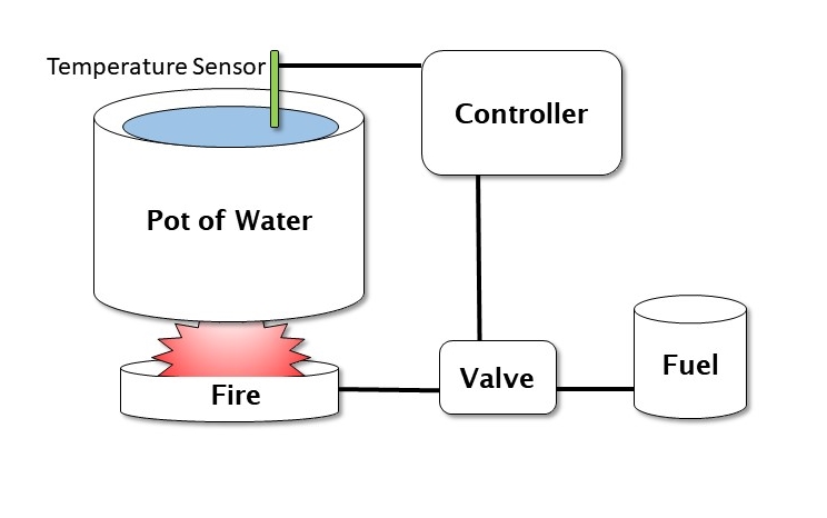
The Valve controls the heat produced by the fire, which warms the pot of water. The Temperature Sensor detects if the water is too cold, too hot, or just right. The Controller uses this information to control the valve for more heat. This type of schema is called a closed loop control system.

You can think of this also in terms of a process. We start the process, and then get feedback to show our progress, so that we know when to stop or modify the process. We could be doing speed control, where we need the robot to move at a specific speed, or pointing control, where the robot aims or turns in a specific direction.

Let’s look at another example. We have a robot with a self-charging docking station, with a set of light emitting diodes (LEDs) on the top as an optical target. We want the robot to drive straight into the docking station. We use the camera to see the target LEDs on the docking station. The camera generates an error, which is the direction that the LEDs are seen in the camera. The distance between the LEDs also gives us a rough range to the dock. Let’s say that the LEDs in the image are off to the left of center 50% and the distance is 3 feet (1 m) We send that information to a control loop to the motors – turn right (opposite the image) a bit and drive forward a bit. We then check again, and the LEDs are closer to the center (40%) and the distance is a bit less (2.9 feet or 90 cm). Our error signal is a bit less, and the distance is a bit less, so we send a slower turn and a slower movement to the motors at this update cycle. We end up exactly in the center and come to zero speed just as we touch the docking station. For those people currently saying "But if you use a PID controller …", yes, you are correct, I’ve just described a "P" or proportional control scheme. We can add more bells and whistles to help prevent the robot from overshooting or undershooting the target due to its own weight and inertia, and to damp out oscillations caused by those overshoots.

The point of these examples is to point out the concept of control in a system. Doing this consistently is the concept of real-time control.

In order to perform our control loop at a consistent time interval (or to use the proper term, deterministically), we have two ways of controlling our program execution: soft real time and hard real time.

A hard real-time system places requirements that a process executes inside a time window that is enforced by the operating system, which provides deterministic performance – the process always takes exactly the same amount of time.

The problem we are faced with is that a computer running an operating system is constantly getting interrupted by other processes, running threads, switching contexts, and performing tasks. Your experience with desktop computers, or even smart phones, is that the same process, like starting up a word processor program, always seems to take a different amount of time whenever you start it up, because the operating system is interrupting the task to do other things in your computer.

This sort of behavior is intolerable in a real-time system where we need to know in advance exactly how long a process will take down to the microsecond. You can easily imagine the problems if we created an autopilot for an airliner that, instead of managing the aircraft’s direction and altitude, was constantly getting interrupted by disk drive access or network calls that played havoc with the control loops giving you a smooth ride or making a touchdown on the runway.

A real-time operating system (RTOS) allows the programmers and developers to have complete control over when and how the processes are executing, and which routines are allowed to interrupt and for how long. Control loops in RTOS systems always take the exact same number of computer cycles (and thus time) every loop, which makes them reliable and dependable when the output is critical. It is important to know that in a hard real-time system, the hardware is enforcing timing constraints and making sure that the computer resources are available when they are needed.

We can actually do hard real time in an Arduino microcontroller, because it has no operating system and can only do one task at a time, or run only one program at a time. We have complete control over the timing of any executing program. Our robot will also have a more capable processor in the form of a Raspberry Pi 3 running Linux. This computer, which has some real power, does quite a number of tasks simultaneously to support the operating system, run the network interface, send graphics to the output HDMI port, provide a user interface, and even support multiple users.

Soft real time is a bit more of a relaxed approach. The software keeps track of task execution, usually in the form of frames, which are set time intervals, like the frames in a movie film. Each frame is a fixed time interval, like 1/20 of a second, and the program divides its tasks into parts it can execute in those frames. Soft real time is more appropriate to our playroom cleaning robot than a safety-critical hard real-time system – plus, RTOSs are expensive and require special training. What we are going to do is treat the timing of our control loop as a feedback system. We will leave extra "room" at the end of each cycle to allow the operating system to do its work, which should leave us with a consistent control loop that executes at a constant time interval. Just like our control loop example, we will make a measurement, determine the error, and apply a correction each cycle.

We are not just worried about our update rate. We also have to worry about "jitter", or random variability in the timing loop caused by the operating system getting interrupted and doing other things. An interrupt will cause our timing loop to take longer, causing a random jump in our cycle time. We have to design our control loops to handle a certain amount of jitter for soft real time, but these are comparatively infrequent events.

The process is actually fairly simple in practice. We start by initializing our timer, which needs to be as high a resolution as we can get. We are writing our control loop in Python, so we will use the time.time() function, which is specifically designed to measure our internal program timing performance (set frame rate, do loop, measure time, generate error, sleep for error, loop). Each time we call time.time(), we get a floating point number, which is the number of seconds from the Unix clock.

The concept for this process is to divide our processing into a set of fixed time frames. Everything we do will fit within an integral number of frames. Our basic running speed will process 30 frames per second. That is how fast we will be updating the robot’s position estimate, reading sensors, and sending commands to motors. We have other functions that run slower than the 30 frames, so we can divide them between frames in even multiples. Some functions run every frame (30 fps), and are called and executed every frame. Let’s say that we have a sonar sensor that can only update 10 times a second. We call the read sonar function every third frame. We assign all our functions to be some multiple of our basic 30 fps frame rate, so we have 30, 15, 10, 7.5, 6,5,4.28,2, and 1 frames per second if we call the functions every frame, every second frame, every third frame, and so on. We can even do less that one frame per second – a function called every 60 frames executes once every 2 seconds.

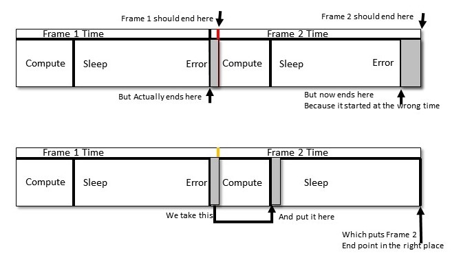
The tricky bit is we need to make sure that each process fits into one frame time, which is 1/30 of a second or 0.033 seconds or 33 milliseconds. If the process takes longer than that, we have to ether divide it up into parts, or run it in a separate thread or program where we can start the process in one frame and get the result in another. It is also important to try and balance the frames so that not all processing lands in the same frame. The following diagram shows a task scheduling system based on a 30 frames per second basic rate.

We have four tasks to take care of: Task A runs at 15 fps, Task B runs at 6 fps (every five frames), Task C runs at 10 fps (every three frames), and Task D runs at 30 fps, every frame. Our first pass (the top diagram) at the schedule has all four tasks landing on the same frame at frames 1, 13, and 25. We can improve the balance of the load on the control program if we delay the start of Task B on the second frame, as shown in the bottom diagram.

This is very akin to how measures in music work, where a measure is a certain amount of time, and different notes have different intervals – one whole note can only appear once per measure, a half note can appear twice, all the way down to 64th notes. Just as a composer makes sure that each measure has the right number of beats, we can make sure that our control loop has a balanced measure of processes to execute each frame.

Let’s start by writing a little program to control our timing loop and to let you play with these principles.

This is exciting; our first bit of coding together. This program just demonstrates the timing control loop we are going to use in the main robot control program, and is here to let you play around with some parameters and see the results. This is the simplest version I think is possible of a soft-time controlled loop, so feel free to improve and embellish.

The following diagram show what we are doing with this program:

Now we begin with coding. This is pretty straightforward Python code; we won't get fancy until later. We start by importing our libraries. It is not surprising that we start with the time module. We also will use the mean function from numpy (Python numerical analysis) and matplotlib to draw our graph at the end. We will also be doing some math calculations to simulate our processing and create a load on the frame rate.

import time
from numpy import mean
import matplotlib.pyplot as plt
import math
#

Now we have some parameters to control our test. This is where you can experiment with different timings. Our basic control is the FRAMERATE – how many updates per second do we want to try? Let’s start with 30, as we did before:

# set our frame rate - how many cycles per second to run our loop?
FRAMERATE = 30
# how long does each frame take in seconds?
FRAME = 1.0/FRAMERATE
# initialize myTimer
# This is one of our timer variables where we will store the clock time from the operating system.
myTimer = 0.0

The duration of the test is set by the counter variable. The time the test will take is the FRAME time times the number of cycles in the counter. In our example, 2000 frames divided by 30 frames per second is 66.6 seconds, or a bit over a minute to run the test:

# how many cycles to test?  counter*FRAME = runtime in seconds
counter = 2000

We will be controlling our timing loop in two ways. We will first measure the amount of time it takes to perform the calculations for this frame. We have a stub of a program with some trig functions we will call to put a load on the computer. Robot control functions, such as computing the angles needed in a robot arm, need lots of trig math to work.

We will measure the time for our control function to run, which will take some part of our frame. We then compute how much of our frame remains, and tell the computer to sleep this process for the rest of the time. Using the sleep function releases the computer to go take care of other business in the operating system, and is a better way to mark time rather that running a tight loop of some sort to waste the rest of our frame time. The second way we control our loop is by measuring the complete frame – compute time plus rest time – and looking to see if we are over or under our frame time. We use TIME_CORRECTION for this function to trim our sleep time to account for variability in the sleep function and any delays getting back from the operating system:

# factor for our timing loop computations
TIME_CORRECTION= 0.0
# place to store data

We will collect some data to draw a "jitter" graph at the end of the program. We use the dataStore structure for this. Let's put a header on the screen to tell the you the program has begun, since it takes a while to finish:

dataStore = []
# Operator information  ready to go
# We create a heading to show that the program is starting its test
print "START COUNTING: FRAME TIME", FRAME, "RUN TIME:",FRAME*counter
# initialize the precision clock

In this step, we are going to set up some variables to measure our timing. As we mentioned, the objective is to have a bunch of compute frames, each the same length. Each frame has two parts: a compute part, where we are doing work, and a sleep period, when we are allowing the computer to do other things. myTime is the "top of frame" time, when the frame begins. newTime is the end of the work period timer. We use masterTime to compute the total time the program is running:

 myTime = newTime = time.time()
 # save the starting time for later
 masterTime=myTime
 # begin our timing loop
 for ii in range(counter):

This section is our "payload", the section of the code doing the work. This might be an arm angle calculation, a state estimate, or a command interpreter. We'll stick in some trig functions and some math to get the CPU to do some work for us. Normally, this "working" section is the majority of our frame, so let's repeat these math terms 1,000 times:

 # we start our frame - this represents doing some detailed math calculations
 # this is just to burn up some CPU cycles
 for jj in range(1000):
 x = 100
 y = 23 + ii
 z = math.cos(x)
 z1 = math.sin(y)
 #
 # read the clock after all compute is done
 # this is our working frame time
 #
 

Now we read the clock to find the working time. We can now compute how long we need to sleep the process before the next frame. The important part is that working time + sleep time = frame time. I'll call this timeError:

 newTime = time.time()
 # how much time has elapsed so far in this frame
 # time = UNIX clock in seconds
 # so we have to subract our starting time to get the elapsed time
 myTimer = newTime-myTime
 # what is the time left to go in the frame?
 timeError = FRAME-myTimer
 

We carry forward some information from the previous frame here. TIME_CORRECTION is our adjustment for any timing errors in the previous frame time. We initialized it earlier to zero before we started our loop so we don't get an undefined variable error here. We also do some range checking because we can get some large "jitters" in our timing caused by the operating system that can cause our sleep timer to crash if we try to sleep a negative amount of time:

 # OK time to sleep
 # the TIME CORRECTION helps account for all of this clock reading
 # this also corrects for sleep timer errors
 # we are using a porpotional control to get the system to converge
 # if you leave the divisor out, then the system oscillates out of control
 sleepTime = timeError + (TIME_CORRECTION/1.5)
 # quick way to eliminate any negative numbers
 # which are possible due to jitter
 # and will cause the program to crash
sleepTime=max(sleepTime,0.0)

So here is our actual sleep command. The sleep command does not always provide a precise time interval, so we will be checking for errors:

 # put this process to sleep
 time.sleep(sleepTime)

This is the time correction section. We figure out how long our frame time was in total (working and sleeping) and subtract it from what we want the frame time to be (FrameTime). Then we set our time correction to that value. I'm also going to save the measured frame time into a data store so we can graph how we did later, using matplotlib. This technique is one of Python's more useful features:

 #print timeError,TIME_CORRECTION
 # set our timer up for the next frame
 time2=time.time()
 measuredFrameTime = time2-myTime
 ##print measuredFrameTime,
 TIME_CORRECTION=FRAME-(measuredFrameTime)
 dataStore.append(measuredFrameTime*1000)
 #TIME_CORRECTION=max(-FRAME,TIME_CORRECTION)
 #print TIME_CORRECTION
 myTime = time.time()

This completes the looping section of the program. This example does 2,000 cycles of 30 frames a second and finishes in 66.6 seconds. You can experiment with different cycle times and frame rates.

Now that we have completed the program, we can make a little report and a graph. We print out the frame time and total runtime, compute the average frame time (total time/counter), and display the average error we encountered, which we can get by averaging the data in the dataStore:

# Timing loop test is over - print the results
#
# get the total time for the program
endTime = time.time() - masterTime
# compute the average frame time by dividing total time by our number of frames
avgTime = endTime / counter
#print report
 print "FINISHED COUNTING"
 print "REQUESTED FRAME TIME:",FRAME,"AVG FRAME TIME:",avgTime
 print "REQUESTED TOTAL TIME:",FRAME*counter,"ACTUAL TOTAL TIME:", endTime
 print "AVERAGE ERROR",FRAME-avgTime, "TOTAL_ERROR:",(FRAME*counter) - endTime
 print "AVERAGE SLEEP TIME: ",mean(dataStore),"AVERAGE RUN TIME",(FRAME*1000)-mean(dataStore)
 # loop is over, plot result
 # this let's us see the "jitter" in the result
 plt.plot(dataStore)
 plt.show()

Results from our program are shown in the following code. Note that the average error is just 0.00018 of a second, or .18 milliseconds out of a frame of 33 milliseconds:

START COUNTING: FRAME TIME 0.0333333333333 RUN TIME: 66.6666666667
FINISHED COUNTING
REQUESTED FRAME TIME: 0.0333333333333 AVG FRAME TIME: 0.0331549999714
REQUESTED TOTAL TIME: 66.6666666667 ACTUAL TOTAL TIME: 66.3099999428
AVERAGE ERROR 0.000178333361944 TOTAL_ERROR: 0.356666723887
AVERAGE SLEEP TIME:  33.1549999714 AVERAGE RUN TIME 0.178333361944

The following diagram shows the timing graph from our program. The "spikes" in the image are jitter caused by operating system interrupts. You can see the program controls the frame time in a fairly narrow range. If we did not provide control, the frame time would get greater and greater as the program executed. The diagram shows that the frame time stays in a narrow range that keeps returning to the correct value:

Now that we have exercised our programming muscles, we can apply this knowledge into the main control loop for our robot. The control loop has two primary functions:

• To respond to commands from the control station
• To interface to the robot's motors and sensors in the Arduino Mega

We will use a standard format for sending commands around the robot. All robot commands will have a three letter identifier, which is just a three letter code that identifies the command. We will use "DRV" for motor drive commands to the tracks, "ARM" for commands to the robot arm, and "TLn" for telemetry data (where "n" is a number or letter, allowing us to create various telemetry lists for different purposes). Error messages will start with "ERR", and general commands will start with "COM". A motor telemetry message might look like this:

TL11500,1438\n

Here TL1 is the identifier (telemetry list 1) and the data is separated by commas. In this case, the two values are the motor states of the left and right drive motors. The \n is the end of line character escape character in Python, which designates the end of that message.

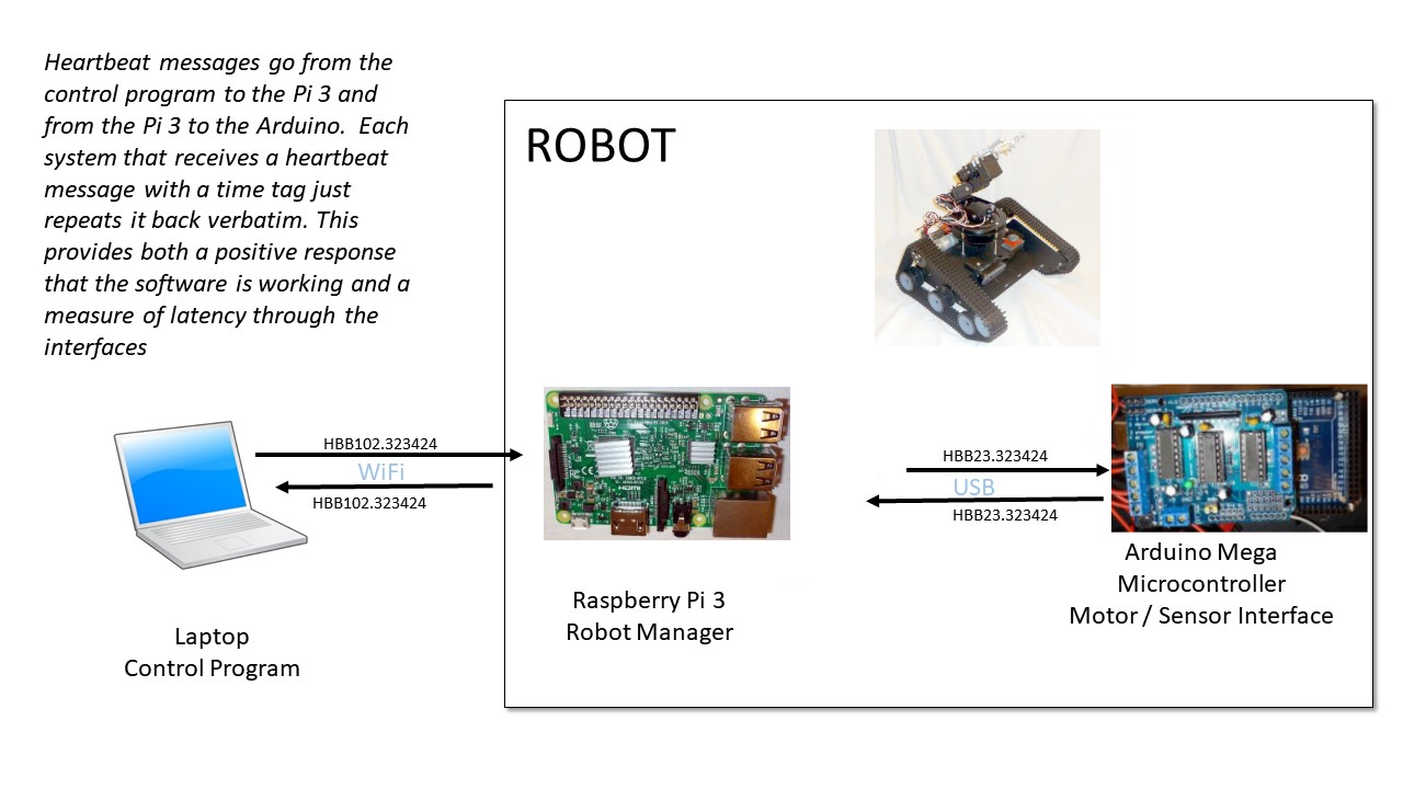
We will also be adding a feature that I always include in all of my robots and unmanned vehicles. It is always good to maintain "positive control" over the robot at all times. We don't want a hardware fault or a software error to result in the robot being stuck in a loop or run out of control. One of the means we can use to detect faults is to use end-to-end heartbeats. A heartbeat is a regular message that is periodically passed from the control station, to the robot's brain, and down to the microcontroller, and then back again. One of the tricks I use is to put a time tag on the heartbeat message so that it also acts as a latency measurement. Latency is the delay time that it takes from the time a command is generated until the robot acts on that command. If we have a heartbeat failure, we can detect that a process is stuck and stop the robot from moving, as well as send an error message to the operator.

This robot, like most of my creations, is designed to run autonomously a majority of the time, so it does not require communications with a control station full time. You can log onto the robot, send some commands, or operate it as a teleoperated unit, and then put it back into autonomous mode. So we have to design the heartbeat to not require a control station, but allow for heartbeats to and from a control station if one is connected.

Twice a second the main computer, the Raspberry Pi3, will send a message with a header of HBB, along with the clock time. The Arduino will simply repeat the HBB message back to the Pi3 with the same time information; that is, it just repeats the message back as soon as it can. This allows the Pi3 to measure the route trip delay time by looking at its clock. Repeating the clock eliminates the problem of synchronizing the clocks on the two systems. When a control program running on my PC is connected to the robot, a separate HBB message comes via the ROS message interface on a special topic called robotCommand, which is just a string message type. The command station puts a time tag on the heartbeat message, which allows the network latency along the wireless (Wi-Fi) network to be measured. Once a command station connects to the robot, it sends a HBB message once a second to the Pi 3 using ROS. The robot just repeats the message back as fast as it can. This tells the control station that the robot is being responsive, and tells the robot that someone is connected via Wi-Fi and is monitoring and can send commands.

Here is a diagram explaining the process:

OK, now let's start into our main robot control program that runs on the Raspberry Pi3 and handles the main controls of the robot, including accepting commands, sending instructions to the motors, receiving telemetry from the Arduino, and keeping the robot's update rate managed:

import rospy
import tf.transformations
from geometry_msgs.msg import Twist
from std_msgs.msg import String
import time
import serial
#GLOBAL VARIABLES
# set our frame rate - how many cycles per second to run our loop?
FRAMERATE = 30
# how long does each frame take in seconds?
FRAME = 1.0/FRAMERATE
# initialize myTimer
topOfFrame = 0.0
endOfWork = 0.0
endOfFrame=0.0
# how many cycles to test? counter*FRAME = runtime in seconds
counter = 2000
# fudge factor for our timing loop computations
TIME_CORRECTION= 0.0
class RosIF():
 def __init__(self):
 self.speed = 0.0
 self.turn = 0.0
 self.lastUpdate = 0.0
 rospy.init_node('robotControl', anonymous=True)
 rospy.Subscribe("cmd_vel",Twist,self.cmd_vel_callback)
 rospy.Subscribe("robotCommand",String,self.robCom_callback)
 self.telem_pub = rospy.Publish("telemetry",String,queue_size=10)
 self.robotCommand=rospy.Publish("robotCommand",String,queue_size=10)
 
 def cmd_vel_callback(self,data):
 self.speed = data.linear.x
 self.turn = data.angular.z
 self.lastUpdate = time.time()
 
 def command(self,cmd):
 rospy.loginfo(cmd)
 self.robotCommand.Publish(cmd)
 def robCom_callback(self,cmd):
 rospy.loginfo(cmd)
 robot_command = cmd.data
 # received command for robot - process
 if robot_command == "STOP":
 robot.stop()
 if robot_command == "GO":
 robot.go()
# This object encapsulates our robot
class Robot():
 def __init__(self):
 # position x,y
 # velocity vx, vy
 # accelleration ax, ay
 # angular position (yaw), angular velocity, angular acceleration
<< CODE SNIPPED - SEE APPENDIX>>

We will cover the design of the robot object in the Appendix. The full code is available in the repository on GitHub. Since we are not using this part of the program for the example in this chapter, I'm going to snip this bit out. See the Appendix; we will be using this section in great detail in later chapters.

One of our functions for the robot control program is to communicate with the Arduino microcontroller over a serial port. How do we do that and maintain our timing loop we have worked so hard for? Let's put down another very important rule about controlling robots that will be illustrated in the next bit of code. Let's make this a tip:

Let's have a quick review. A blocking call suspends execution of our program to wait for some event to happen. In this case, we would be waiting for the serial port to receive data ending in a new line character. If the system on the other end of the serial port never sends data, we can be blocked forever, and our program will freeze. So how do we talk to our serial port? We poll the port (examine the port to see if data is available), rather than wait for data to arrive, which would the be standard manner to talk to a serial port. That means we use read instead of readline commands, since readline blocks (suspends our execution) until a newline character is received. That means we can't count on the data in the receive buffer to consist only of complete lines of data. We need to pull the data until we hit a newline character (\n in Python), then put that data into our dataline output buffer (see the following code), and process it. Any leftover partial lines we will save for later, when more data is available. It's a bit more work, but the result is that we can keep our timing.

For advanced students, it is possible to put the read serial function into a separate thread and pass the data back and still use a blocking call, but I think this is just as much work as what we are doing here, and the polling technique is less overhead for the processor and more control for us, because we are never blocked:

def readBuffer(buff):
# the data we get is a series of lines separated by EOL symbols
# we read to a EOL character (0x10) that is a line
# process complete lines and save partial lines for later
# 
EOL = '\n'
if len(buff)==0:
    return
dataLine = ""
lines=[]
for inChar in buff:
    if inChar != EOL:
    dataLine +=inChar
else:
    lines.append(dataLine)
    dataLine=""
for telemetryData in lines:
    processData(telemetryData)
return dataLine

This part of the code processes the complete lines of data we get from the Arduino. We have three types of message we can get from the microcontroller. Each message starts with a three letter identifier followed by data. The types are HBB for heartbeat, TLn for telemetry, and ERR for error messages. Right now we just have one telemetry message, TL1 (telemetry list 1). Later we will add more telemetry lists as we add sensors to the robot. The HBB message is just the Arduino repeating back the heartbeat message we send it twice a second. We'll use ERR to send messages back to the control program from the microcontroller, and these will be things like illegal motor command:

def processData(dataLine):
 #
 # take the information from the arduino and process telemetry into
 # status information
 # we recieve either heartbeat (HBB), TL1 (telemtry List 1), or ERR (Error messages)
 # we are saving room for other telemetry lists later
 dataType = dataLine[:3]
 payload = dataLine[3:] # rest of the line is data
 if dataType == 'HBB':
 # process heartbeat
 # we'll fill this in later
 pass
 if dataType == "TL1": # telemetry list 1
 # we'll add this later
 pass
 if dataType == "ERR": # error message
 print "ARUDUINO ERROR MESSAGE ",payload
 # log the error
 rospy.loginfo(payload)
 return
 

This section starts our main program. We start by instantiating our objects for the ROS interface and the robot. I like to put the ROS interface stuff in an object because it makes it easier to keep track of and make changes. Then, we open the serial port to the Arduino on /dev/ttyUSB0. Note that we set the timeout to zero. I don't think this is relevant since we are not using blocking calls on the serial port, but it can't hurt to double check that no blocking takes place. We do some error checking with the try...except block to catch any errors. Since the lack of a connection to the robot motors means we can't operate at all, I've had the program raise the error and stop the program run:

# main program starts here
# *****************************************************
rosif = RosIF() # create a ROS interface instance
robot = Robot() # define our robot instance
serialPort = "/dev/ttyUSB0"
# open serial port to arduino
ser = serial.Serial(serialPort,38400,timeout=0) #
# serial port with setting 38,400 baud, 8 bits, No parity, 1 stop bit
try:
 ser.open()
except:
 print "SERIAL PORT FOR ARDIONO DID NOT OPEN ", serialPort
 raise

Now, we start the ROS loop. not rospy.is_shutdown() controls the program and allows us to use the ROS shutdown command to terminate the program. We also initialize our frame counter we use to schedule tasks. I count the frames in each second (frameKnt) and then can set tasks to run at some divisor of the frame rate, as we discussed earlier in the chapter:

 frameKnt = 0 # counter used to time processes
 while not rospy.is_shutdown():
 # main loop
 topOfFrame=time.time()
 # do our work
 # read data from the seral port if there is any
 serData = ser.read(1024)
 # process the data from the arduino
 # we don't want any blocking, so we use read and parse the lines ourselves
 holdBuffer = readBuffer(serData)
 #drive command
 com = ',' # comma symbol we use as a separator
 EOL = '\n'
 if robot.newCommand:
 ardCmd = "DRV"+str(robot.leftMotorCmd)+com+str(robot.rightMotorCmd)+EOL
 serial.write(ardCmd)
 serial.flush() # output Now

Here is an example of scheduling a task. We want the heartbeat message to go to the Arduino twice a second, so we compute how many frames that is (15 in this case) and then use the modulo operator to determine when that occurs. We use the formula in case we want to change the frame rate later, and we probably will.:

 if frameKnt % (FRAMERATE/2)==0: # twice per second
 hbMessage = "HBB"+com+str(time.time())+EOL
 serial.write(hbMessage)
 serial.flush() # output Now

We manage the frame counter, resetting it each second back to zero. We could let it just run, but let's keep it tidy. We'll reset the frame counter each second so we don't have to worry about overflow later:

 frameKnt +=1
 if frameKnt > FRAMERATE: frameKnt = 0 # just count number of frames in a second
 
 # done with work, now we make timing to get our frame rate to come out right
 #
 endOfWork = time.time()
 workTime = endOfWork - topOfFrame
 sleepTime = (FRAME-workTime)+ timeError
 time.sleep(sleepTime)
 endOfFrame = time.time()
 actualFrameTime = endOfFrame-topOfFrame
 timeError = FRAME-actualFrameTime
 # clamp the time error to the size of the frame
 timeError = min(timeError,FRAME)
 timeError = max(timeError,-FRAME)

Finally, when we fall out of the loop and end the program, we need to close the serial port to prevent the port from being locked the next time we start up:

 # end of the main loop
 #
 ser.close()

In this chapter, we introduced the subject of artificial intelligence, and discussed that this is an artificial intelligence book applied to robotics, so our emphasis will be on AI. The main difference between an AI robot and a "regular" robot is that an AI robot may behave non-deterministically, which is to say it may have a different response to the same stimulus, due to learning. We introduced the problem we will use throughout the book, which is picking up toys in a playroom and putting them into a toy box. Next, we discussed two critical tools for AI robotics: the OODA loop (Observe-Orient-Decide-Act), which provides a model for how our robot makes decisions, and the soft real-time control loop, which manages and controls the speed of execution of our program. We applied these techniques in a timing loop demonstration and began to develop our main robot control program. The Appendix provides detailed instructions on setting up the various environments and software we will use to develop our AI-based robot, which I call TinMan.

1. What does the acronym PID stand for? Is this considered an AI software method?
2. What is the Turing test? Do you feel this is a valid method of assessing an artificial intelligence system?
3. Why do you think robots have a problem in general with negative obstacles, such as stairs and potholes?
4. In the OODA loop, what does the "orient" step do?
5. From the discussion of Python advantages, compute the following. You have a program that needs 50 changes tested. Assuming each change requires one run and a recompile step to test. A "C" Make step takes 450 seconds and a Python "run" command takes 3 seconds. How much time do you sit idle waiting for the C compiler?
6. What does RTOS stand for?

7. Your robot has the following scheduled tasks: telemetry: 10 Hz GPS 5 Hz Inertial 50 Hz Motors 20 Hz. What base frame rate would you use to schedule these tasks? (Hz or hertz means times per second. 3 Hz = three times per second)
8. Given that a frame rate scheduler has the fastest task at 20 frames per second, how would you schedule a task that needs to run at seven frames per second? How about one that runs at 3.5 frames per second?
9. What is a blocking call function? Why is it bad to use blocking calls in a real-time system like a robot?

• Coram, R. (2004). Boyd: The Fighter Pilot Who Changed the Art of War. New York, NY: Back Bay Books/Little, Brown. (History of the OODA Loop)
• Fernández, E., Crespo, L. S., Mahtani, A., and Martinez, A. (2015). Learning ROS for Robotics Programming: Your One-Stop Guide to the Robot Operating System. Birmingham, UK: Packt Publishing.
• Joshi, P. (2017). Artificial Intelligence with Python: A Comprehensive Guide to Building Intelligent Apps for Python Beginners and Developers. Birmingham, UK: Packt Publishing Ltd.
• Brooks, R. (1986). "A robust layered control system for a mobile robot". Robotics and Automation, IEEE Journal of . 2 (1): 14–23. doi:10.1109/JRA.1986.1087032.