


Note
Learning Objectives
By the end of this chapter, you will be able to:
Present data for use in machine learning models
Explain how to preprocess data for a machine learning model
Build a logistic regression model with scikit-learn
Use regularization in machine learning models
Evaluate model performance with model evaluation metrics
Machine learning is the science of utilizing machines to emulate human tasks and to have the machine improve their performance of that task over time. By feeding machines data in the form of observations of real-world events, they can develop patterns and relationships that will optimize an objective function, such as the accuracy of a binary classification task or the error in a regression task. In general, the usefulness of machine learning is in the ability to learn highly complex and non-linear relationships in large datasets and to replicate the results of that learning many times.
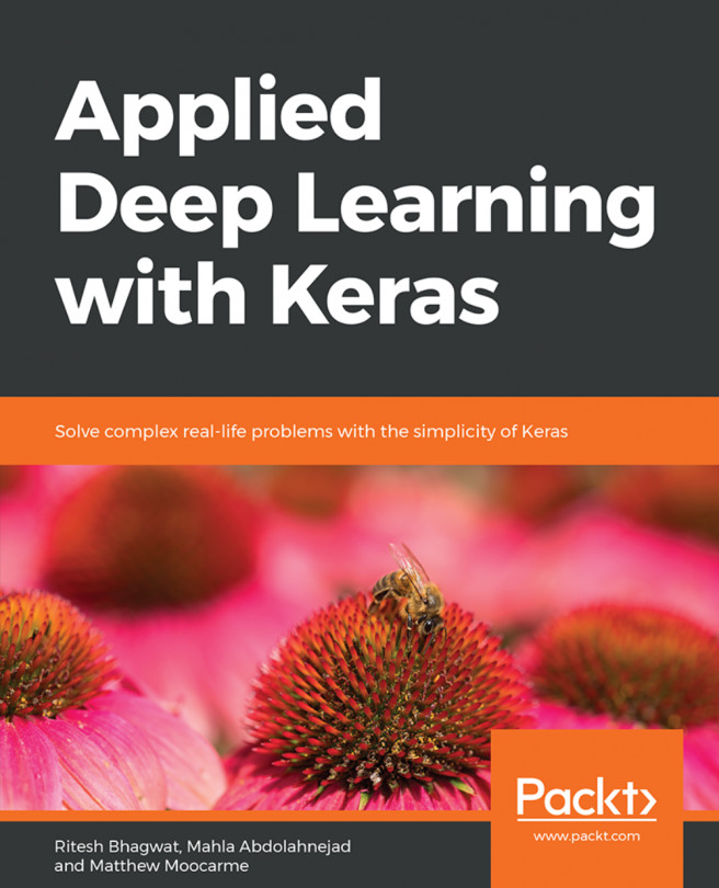
Take, for example, the classification of a dataset of pictures of either dogs or cats into classes of their respective type. For a human, this is trivial, and the accuracy would likely be very high. However, it may take around a second to categorize each picture, and scaling the task can only be achieved by increasing the number of humans, which may be infeasible. While it may be difficult, though certainly not impossible, for machines to reach the same level of accuracy as humans for this task, machines can classify many images per second, and scaling can be easily done by increasing the processing power of single machine, or making the algorithm more efficient.
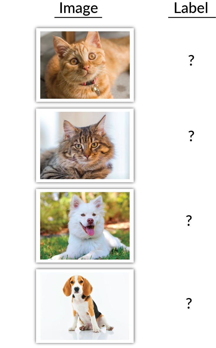
Figure 1.1: A trivial classification task for humans, but quite difficult for machines
While the trivial task of classifying dogs and cats may be simple for us humans, the same principles that are used to create a machine learning model classify dogs and cats can be applied to other classification tasks that humans may struggle with. An example of this is identifying tumors in Magnetic Resonance Images (MRIs). For humans, this task requires a medical professional with years of experience, whereas a machine may only need a dataset of labeled images.
Figure 1.2: A non-trivial classification task for humans. Are you able to spot the tumors?
We build models so that we can learn something about the data we are training on and about the relationships between the features of the dataset. This learning can inform us when we encounter new observations. However, we must realize that the observations we interact with in the real world and the format of data needed to train machine learning models are very different. Working with text data is a prime example of this. When we read text, we are able to understand each word and apply context given each word in relation to the surrounding words -- not a trivial task.However, machines are unable to interpret this contextual information. Unless it specifically encoded, they have no idea how to convert text into something that can be an input numerical. Therefore, we must represent the data appropriately, often by converting non-numerical data types, for example, converting text, dates, and categorical variables into numerical ones.
Much of the data fed into machine learning problems is two-dimensional, and can be represented as rows or columns. Images are a good example of a dataset that may be three-or even four-dimensional. The shape of each image will be two-dimensional (a height and a width), the number of images together will add a third dimension, and a color channel (red, green, blue) will add a fourth.

Figure 1.3: A color image and its representation as red, green, and blue images
Note
We have used datasets from this repository: Dua, D. and Graff, C. (2019). UCI Machine Learning Repository [http://archive.ics.uci.edu/ml]. Irvine, CA: University of California, School of Information and Computer Science.
The following figure shows a few rows from a marketing dataset taken from the UCI repository. The dataset presents marketing campaign results of a Portuguese banking institution. The columns of the table show various details about each customer, while the final column, y, shows whether or not the customer subscribed to the product that was featured in the marketing campaign.
One objective of analyzing the dataset could be to try and use the information given to predict whether a given customer subscribed to the product (that is, to try and predict what is in column y for each row). We can then check whether we were correct by comparing our predictions to column y. The longer-term benefit of this is that we could then use our model to predict whether new customers will subscribe to the product, or whether existing customers will subscribe to another product after a different campaign.

Figure 1.4: An image showing the first 20 instances of the marketing dataset
Data can be in different forms and can be available in many places. Datasets for beginners are often given in a flat format, which means that they are two-dimensional, with rows and columns. Other common forms of data may include images, JSON objects, and text documents. Each type of data format has to be loaded in specific ways. For example, numerical data can be loaded into memory using the NumPy library, which is an efficient library for working with matrices in Python. However, we would not be able to load our marketing data .csv into memory using the NumPy library because the dataset contains string values. For our dataset, we will use the pandas library becauseof its ability to easily work with various data types, such as strings, integers, floats, and binary values. In fact, pandas is dependent on NumPy for operations on numerical data types. pandas is also able to read JSON, Excel documents, and databases using SQL queries, which makes the library common amongst practitioners for loading and manipulating data in Python.
Here is an example of how to load a CSV file using the NumPy library. We use the skiprows argument in case is there is a header, which usually contains column names:
import numpy as np
data = np.loadtxt(filename, delimiter=",", skiprows=1)
Here's an example of loading data using the pandas library:
import pandas as pd
data = pd.read_csv(filename, delimiter=",")
Here we are loading in a CSV file. The default delimiter is a comma, and so passing this as an argument is not necessary, but is useful to see. The pandas library can also handle non-numeric datatypes, which makes the library more flexible:
import pandas as pd
data = pd.read_json(filename)
The pandas library will flatten out the JSON and return a DataFrame.
The library can even connect to a database, and queries can be fed directly into the function, and the table returned will be loaded as a pandas DataFrame:
import pandas as pd
data = pd.read_sql(con, "SELECT * FROM table")
We have to pass a database connection to the function in order for this to work. There are a myriad of ways for this to be achieved, depending on the database flavor.
Other forms of data that are common in deep learning, such as images and text, can also be loaded in and will be discussed later in the book.
Note
For all exercises and activities in this chapter, you will need to have Python 3.6, Jupyter, and pandas installed on your system. They are developed in Jupyter notebooks. It is recommended to keep a separate notebook for different assignments. You can download all the notebooks from the GitHub repository. Here is the link: https://github.com/TrainingByPackt/Applied-Deep-Learning-with-Keras.
In this exercise, we will be loading the bank marketing dataset from the UCI Machine Learning Repository. The goal of this exercise will be to load in the CSV data, identify a target variable to predict, and feature variables with which to use to model the target variable. Finally, we will separate the feature and target columns and save them to CSV files to use in subsequent activities and exercises.
The dataset comes from a Portuguese banking institution and is related to direct marketing campaigns by the bank. Specifically, these marketing campaigns were composed of individual phone calls to clients, and the success of the phone call, that is, whether or not the client subscribed to a product. Each row represents an interaction with a client and records attributes of the client, campaign, and outcome. You can look at the bank-names.txt file provided in the bank.zip file, which describes various aspects of the dataset:
Note
The header='y' parameter is used to provide a column name. We will do this to reduce confusion later on.
In this topic, we have successfully demonstrated how to load data into Python using the pandas library. This will form the basis of loading data into memory for most tabular data. Images and large documents, other common forms of data for machine learning applications, have to be loaded in using other methods that are discussed later in the book.
Open a Jupyter notebook from the start menu to implement this exercise.
Download the dataset from https://github.com/TrainingByPackt/Applied-Deep-Learning-with-Keras/tree/master/Lesson01/data.
To verify that the data looks as follows, we can look at the first 10 rows of the .csv file using the head function:
!head data/bank.csv
The output of the preceding code is as follows:
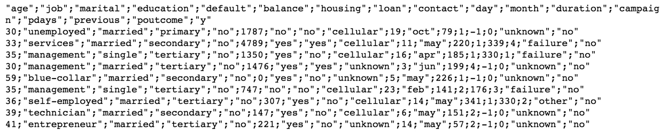
Figure 1.5: The first 10 rows of the dataset
Now let's load the data into memory using the pandas library with the read_csv function. First, import the pandas library:
import pandas as pd
bank_data = pd.read_csv('data/bank.csv', sep=';')
Finally, to verify that we have the data loaded into the memory correctly, we can print the first few rows. Then, print out the top 20 values of the variable:
bank_data.head(20)
The printed output should look like this:

Figure 1.6: The first 20 rows of the pandas DataFrame
We can also print the shape of the DataFrame:
bank_data.shape
The printed output should look as follows, showing that the DataFrame has 4,521 rows and 17 columns:
The following figure shows the output of the preceding code:
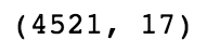
Figure 1.7: Output of the shape command on the DataFrame
We have successfully loaded the data into memory, and now we can manipulate and clean the data so that a model can be trained using this data. Remember that machine learning models require data to be represented as numerical data types in order to be trained. We can see from the first few rows of the dataset that some of the columns are string types, so we will have to convert them to numerical data types later in the chapter.
We can see that there is a given output variable for the dataset, known as 'y', which indicates whether or not the client has subscribed. This seems like an appropriate target to predict for, since it is conceivable that we may know all the variables about our clients, such as their age. For those variables that we don't know, substituting unknowns is acceptable. The 'y' target may be useful to the bank to figure out as to which customers they want to focus their resources on. We can create feature and target datasets as follows, providing the axis=1 argument:
feats = bank_data.drop('y', axis=1) target = bank_data['y']To verify that the shapes of the datasets are as expected, we can print out the number of rows and columns of each:
print(f'Features table has {feats.shape[0]} rows and {feats.shape[1]} columns')print(f'Target table has {target.shape[0]} rows')The following figure shows the output of the preceding code:
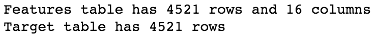
Figure 1.8: Output of the shape commands on the feature and target DataFrames
We can see two important things here that we should always verify before continuing: first, the number of rows of the feature DataFrame and target DataFrame are the same. Here, we can see that both have 4,521 rows. Second, the number of columns of the feature DataFrame should be one fewer than the total DataFrame, and the target DataFrame has exactly one column.
On the second point, we have to verify that the target is not contained in the feature dataset, otherwise the model will quickly find that this is the only column needed to minimize the total error, all the way down to zero. It's also not incredibly useful to include the target in the feature set. The target column doesn't necessarily have to be one column, but for binary classification, as in our case, it will be. Remember that these machine learning models are trying to minimize some cost function, in which the target variable will be part of that cost function.
Finally, we will save our DataFrames to CSV so that we can use them later:
feats.to_csv('data/bank_data_feats.csv')target.to_csv('data/bank_data_target.csv', header='y')
To fit models to the data, it must be represented in numerical format since the mathematics used to in all machine learning algorithms only work on matrices of numbers (you cannot perform linear algebra on an image). This will be one goal of this topic, to learn how to encode all features into numerical representations. For example, in binary text, values that contain one of two possible values may be represented as zeros or ones. An example is shown in the following figure. Since there are only two possible values, a value 0 is assumed to be a cat and the value 1 a dog We can also rename the column for interpretation..
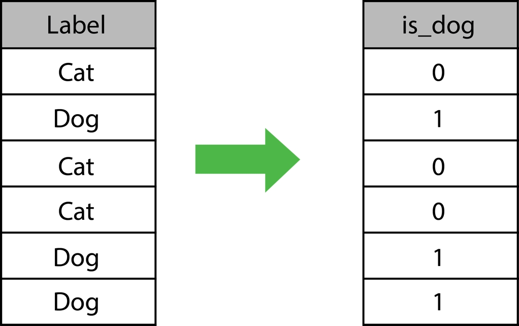
Figure 1.9: A numerical encoding of binary text values
Another goal will be to appropriately represent the data in numerical format — by appropriately, we mean that we want to encode relevant information numerically through the distribution of numbers. For example, one method to encode the months of the year would be to use the number of the month in the year. For example, January would be encoded as 1, since it is the first month, and December would be 12. Here's an example of how this would look in practice:
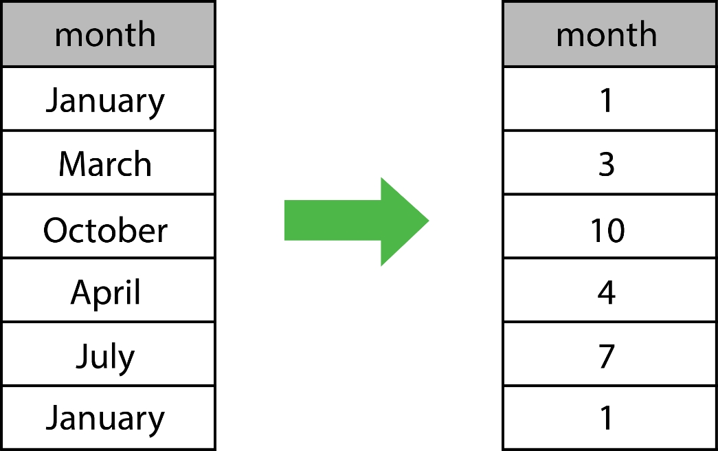
Figure 1.10: A numerical encoding of months
Not encoding information appropriately into numerical features can lead to machine learning models learning unintuitive representations, and relationships between the feature data and target variables that will prove useless for human interpretation.
An understanding of the machine learning algorithms you are looking to use will also help encode features into numerical representations appropriately. For example, algorithms for classification tasks such as Artificial Neural Networks (ANNs) and logistic regression are susceptible to large variations in the scale between the features that may hamper model-fitting ability. Take, for example, a regression problem attempting to fit house attributes, such as area in square feet and the number of bedrooms, to the house price. The bounds of the area may be anywhere from 0 to 5,000, whereas the number of bedrooms may only vary from 0 to 6, so there is a large difference between the scale of the variables. An effective way to combat the large variation in scale between the features is to normalize the data. Normalizing the data will scale the data appropriately so that it is all of a similar magnitude, so that any model coefficients or weights can be compared correctly. Algorithms such as decision trees are unaffected by data scaling, so this step can be omitted for models using tree-based algorithms.
In this topic, we demonstrate a number of different ways to encode information numerically. There is a myriad of alternative techniques that can be explored elsewhere. Here, we will show some simple and popular methods to tackle common data formats.
It is important that we clean the data appropriately so that it can be used for training models. This often includes converting non-numerical datatypes into numerical datatypes. This will be the focus of this exercise – to convert all columns in the feature dataset into numerical columns. To complete the exercise, perform the following steps:
First, we load the feature dataset into memory:
%matplotlib inline import pandas as pd bank_data = pd.read_csv('data/bank_data_feats.csv', index_col=0)Again, we can look at the first 20 rows to check out the data:
bank_data.head(20)
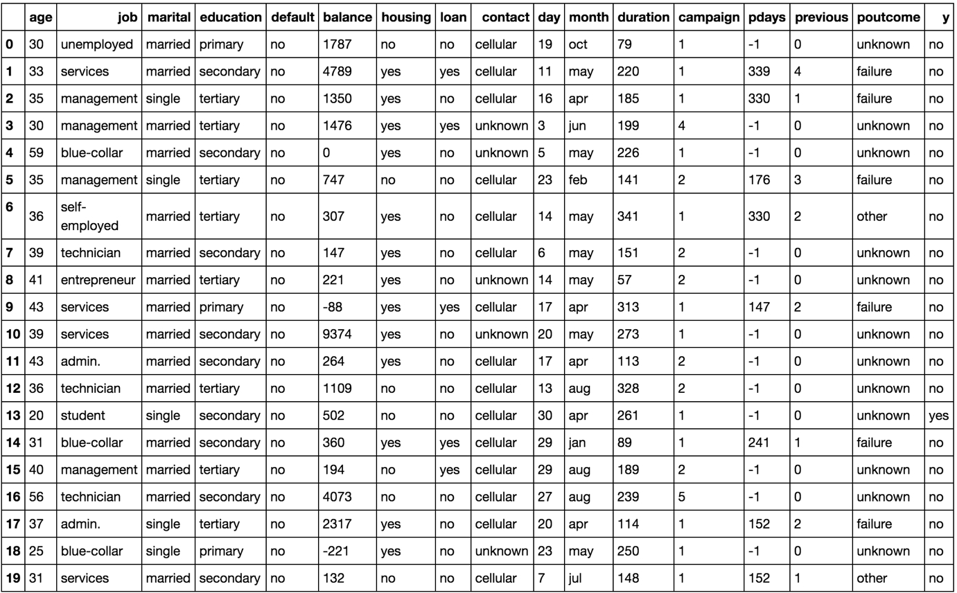
Figure 1.11: First 20 rows of the pandas feature DataFrame
We can see that there are a number of columns that need to be converted to numerical format. The numerical columns we may not need to touch the columns named age, balance, day, duration, campaign, pdays, and previous.
There are some binary columns, which have either one of two possible values. They are default, housing, and loan.
Finally, there are also categorical columns that are string types, but there are a limited number of choices (>2) that the column can take. They are job, education, marital, contact, month, and poutcome.
For the numerical columns, we can use the describe function, which can give us a quick indication of the bounds of the numerical columns:
bank_data.describe()
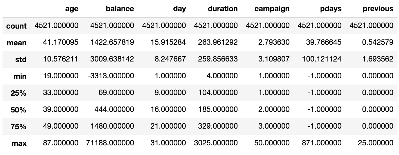
Figure 1.12: Output of the describe function in the feature DataFrame
We will convert the binary columns into numerical columns. For each column, we will follow the same procedure, examine the possible values, and convert one of the values to 1 and the other to 0. If appropriate, we will rename the column for interpretability.
For context, it is helpful to see the distribution of each value. We can do that using the value_counts function. We can try this out on the default column:
bank_data['default'].value_counts()
We can also look at these values as a bar graph by plotting the value counts:
bank_data['default'].value_counts().plot(kind='bar')
Note
The kind='bar' argument will plot the data as a bar graph. The default is a line graph. When plotting in the Jupyter Notebook, in order to make the plots within the notebook, the following command may need to be run: %matplotlib inline.
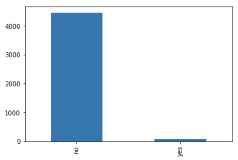
Figure 1.13: A plot of the distribution of values of the default column
We can see that this distribution is very skewed. Let's convert the column to numerical value by converting the yes values to 1, and the no values to 0. We can also change the name of the column from default to is_default. This makes it a bit more obvious what the column means:
bank_data['is_default'] = bank_data['default'].apply(lambda row: 1 if row == 'yes' else 0)
We can take a look at the original and converted columns side by side. We can take a sample of the last few rows to show examples of both values manipulated to numerical data types:
bank_data[['default','is_default']].tail()
Note
The tail function is identical to the head function, except the function returns the bottom n values of the DataFrame instead of the top n.
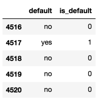
Figure 1.14: The original and manipulated default column
We can see that yes is converted to 1 and no is converted to 0.
Let's do the same for the other binary columns, housing and loan:
bank_data['is_loan'] = bank_data['loan'].apply(lambda row: 1 if row == 'yes' else 0)
bank_data['is_housing'] = bank_data['housing'].apply(lambda row: 1 if row == 'yes' else 0)
Next, we have to deal with categorical columns. We will approach the conversion of categorical columns to numerical values slightly differently, than with binary text columns but the concept will be the same. We will convert each categorical column into a set of dummy columns. With dummy columns, each categorical column will be converted to n columns, where n is the number unique values in the category. The columns will be zero or one depending on the value of categorical column.
This is achieved with the get_dummies function. If we need any help understanding the function, we can use the help function, or any function:
help(pd.get_dummies)
Figure 1.15: The output of the help command applied to the pd.get_dummies function
Let's demonstrate how to manipulate categorical columns with the marital column. Again, it is helpful to see the distribution of values, so let's look at the value counts and plot them:
bank_data['marital'].value_counts()
bank_data['marital'].value_counts().plot(kind='bar')
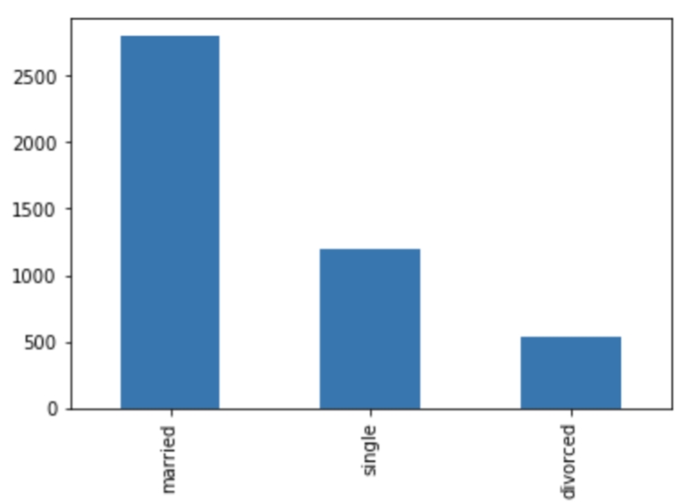
Figure 1.16: A plot of the distribution of values of the marital column
We can call the get_dummies function on the marital column and take a look at the first few rows alongside the original:
marital_dummies = pd.get_dummies(bank_data['marital'])
pd.concat([bank_data['marital'], marital_dummies], axis=1).head(n=10)
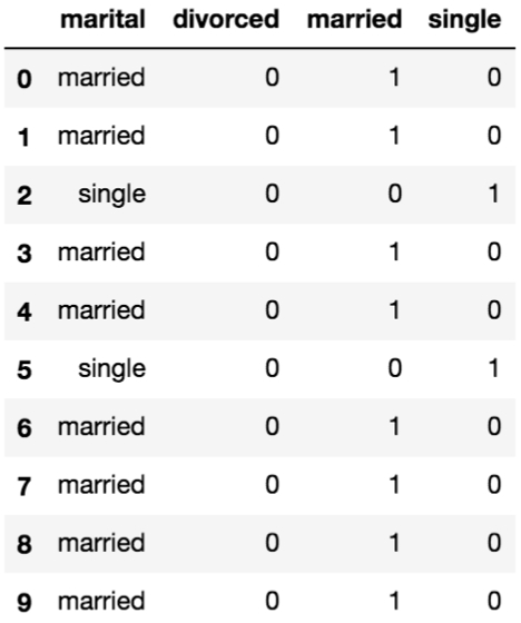
Figure 1.17: Dummy columns from the marital column
We can see that in each of the rows there can be one value of 1, which is in the column corresponding the value in the marital column.
In fact, when using dummy columns there is some redundant information. Because we know there are three values, if two of the values in the dummy columns are zero for a particular row, then the remaining column must be equal to one. It is important to eliminate any redundancy and correlations in features as it becomes difficult to determine which feature is most important in minimizing the total error.
To remove the inter-dependency, let's drop the divorced column because it occurs with the lowest frequency. We can also change the name of the columns so that it is a little easier to read and include the original column:
marital_dummies.drop('divorced', axis=1, inplace=True)
marital_dummies.columns = [f'marital_{colname}' for colname in marital_dummies.columns]
marital_dummies.head()
Note
In the drop function, the inplace argument will apply the function in place, so a new variable does not have to declared.
Looking at the first few rows, we can see what remains of our dummy columns for the original marital column.
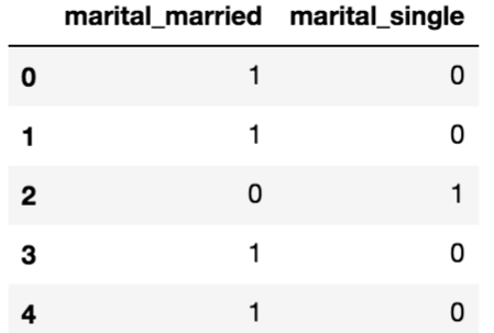
Figure 1.18: Final dummy columns from the marital column
Finally, we can add these dummy columns to the original feature data by concatenating the two DataFrames column-wise and dropping the original column:
bank_data = pd.concat([bank_data, marital_dummies], axis=1)
bank_data.drop('marital', axis=1, inplace=True)
We will repeat the exact same steps with the remaining categorical columns: education, job, contact, and poutcome. First, we will examine the distribution of column values, which is an optional step. Second, we will create dummy columns. Third, we will drop one of the columns to remove redundancy. Fourth, we will change the column names for interpretability. Fifth, we will concatenate the dummy columns into a feature dataset. Sixth, we will drop the original column if it remains in the dataset.
We could treat the month column like a categorical variable, although since there is some order to the values (January comes before February, and so on) they are known as ordinal values. We can encode this into the feature by converting the month name into the month number, for example, January becomes 1 as it is the first month in the year.
This is one way to convert months into numerical features that may make sense in certain models. In fact, for a logistic regression model, this may not make sense since we are encoding some inherent weighting into the features. This feature will contribute 12 times as much for rows with December as the month compared to January, which there should be no reason to do. Regardless, in the spirit of showing multiple techniques to convert columns to numerical datatypes, we will continue.
We can achieve this result by mapping the month names to month numbers by creating a Python dictionary of key-value pairs in which the keys will be the month names and the values will be the month numbers:
month_map = {'jan':1, 'feb':2, 'mar':3, 'apr':4, 'may':5, 'jun':6, 'jul':7, 'aug':8, 'sep':9, 'oct':10, 'nov':11, 'dec': 12}Then we can convert the column by utilizing the map function:
bank_data['month'] = bank_data['month'].map(month_map)
Since we have kept the column name the same, there is no need for us to concatenate back into the original feature dataset and drop the column.
Now we should have our entire dataset as numerical columns. Let's check the types of each column to verify:
bank_data.dtypes
Figure 1.19: The datatypes of the processed feature dataset
Now that we have verified the datatypes, we have a dataset we can use to train a model, so let's save this for later:
bank_data.to_csv('data/bank_data_feats_e2.csv')Let's do the same for the target variable. First, load the data in, then convert the column to numerical datatype, and lastly, save the column as CSV:
target = pd.read_csv('data/bank_data_target.csv', index_col=0)
target.head(n=10)
Figure 1.20: First 10 rows of the target dataset
We can see that this is a string datatype, and there are two unique values.
Let's convert this into a binary numerical column, much like we did the binary columns in the feature dataset:
target['y'] = target['y'].apply(lambda row: 1 if row=='yes' else 0)
target.head(n=10)
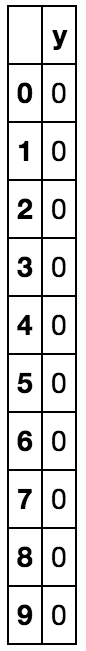
Figure 1.21: First 10 rows of the target dataset when converted to integers
Finally, we save the target dataset to CSV:
target.to_csv('data/bank_data_target_e2.csv')
In this exercise, we learned how to clean the data appropriately so that it can be used to train models. We converted the non-numerical datatypes into numerical datatypes. That is, we converted all the columns in the feature dataset into numerical columns. Lastly, we saved the target dataset to a CSV file so that we can use them in the succeeding exercises or activities.
In our bank marketing dataset, we have some columns that do not appropriately represent the data, which will have to be addressed if we want the models we build to learn useful relationships between the features and the target. One column that is an example of this is the pdays column. In the documentation, the column is described as follows:
pdays: number of days that passed by after the client was last contacted from a previous campaign (numeric, -1 means client was not previously contacted)
Here we can see that a value of -1 means something quite different than a positive number. There are two pieces of information encoded in this one column that we may want to separate. They are as follows:
Whether or not they were contacted
If they were contacted, how long ago was that last contact made
When we create columns, they should ideally align with hypotheses we create of relationships between the features and the target.
One hypothesis may be that previously contacted customers are more likely to subscribe to the product. Given our column, we could test this hypothesis by converting the pdays column into a binary variable indicating whether they were previously contacted or not. This can be achieved by observing whether the value of pdays is -1. If so, we will associate that with a value of 0; otherwise, they have been contacted, so the value will be 1.
A second hypothesis is that the more recently the customer was contacted, the greater the likelihood that they will subscribe. There are many ways to encode this second hypothesis. I recommend encoding the first one, and if we see that this feature has predictive power, we can implement the second hypothesis.
Since building machine learning models is an iterative process, we can choose either or both hypotheses and evaluate whether their inclusion has increased the model's predictive performance.
In this exercise, we will encode the hypothesis that a customer will be more likely to subscribe to the product that they were previously targeted with. We will encode this hypothesis by transforming the pdays column. Wherever the value is -1, we will transform it to 0, indicating the customer has never been previously contacted. Otherwise, the value will be 1. To do so, we follow the following steps:
Open a Jupyter notebook.
Load the dataset into memory. We can use the same feature dataset as was the output from Exercise 2:
import pandas as pd
bank_data = pd.read_csv('data/bank_data_feats_e2.csv', index_col=0)
Use the apply function to manipulate the column and create a new column:
bank_data['was_contacted'] = bank_data['pdays'].apply(lambda row: 0 if row == -1 else 1)
Drop the original column:
bank_data.drop('pdays', axis=1, inplace=True)Let's look at the column that was just changed:
bank_data[['was_contacted']].head(n=10)
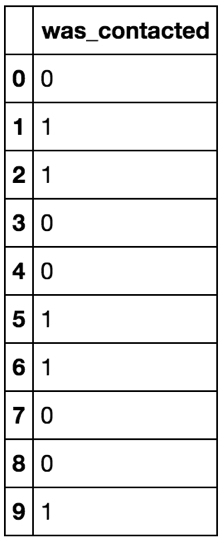
Figure 1.22: The first 10 rows of the formatted column
Finally, let's save the dataset to a CSV file for later use:
bank_data.to_csv('data/bank_data_feats_e3.csv')
Great! Now we can test our hypothesis of whether previous contact will affect the target variable. This exercise has demonstrated how to appropriately represent data for use in machine learning algorithms. We have presented some techniques to convert data into numerical datatypes that cover many situations that may be encountered when working with tabular data.
In this section, we will cover the life cycle of creating performant machine learning models from engineering features, to fitting models to training data, and evaluating our models using various metrics. Many of the steps to create models are highly transferable between all machine learning libraries – we'll start with scikit-learn, which has the advantage of being widely used, and as such there is a lot of documentation, tutorials, and learning to be found across the internet.
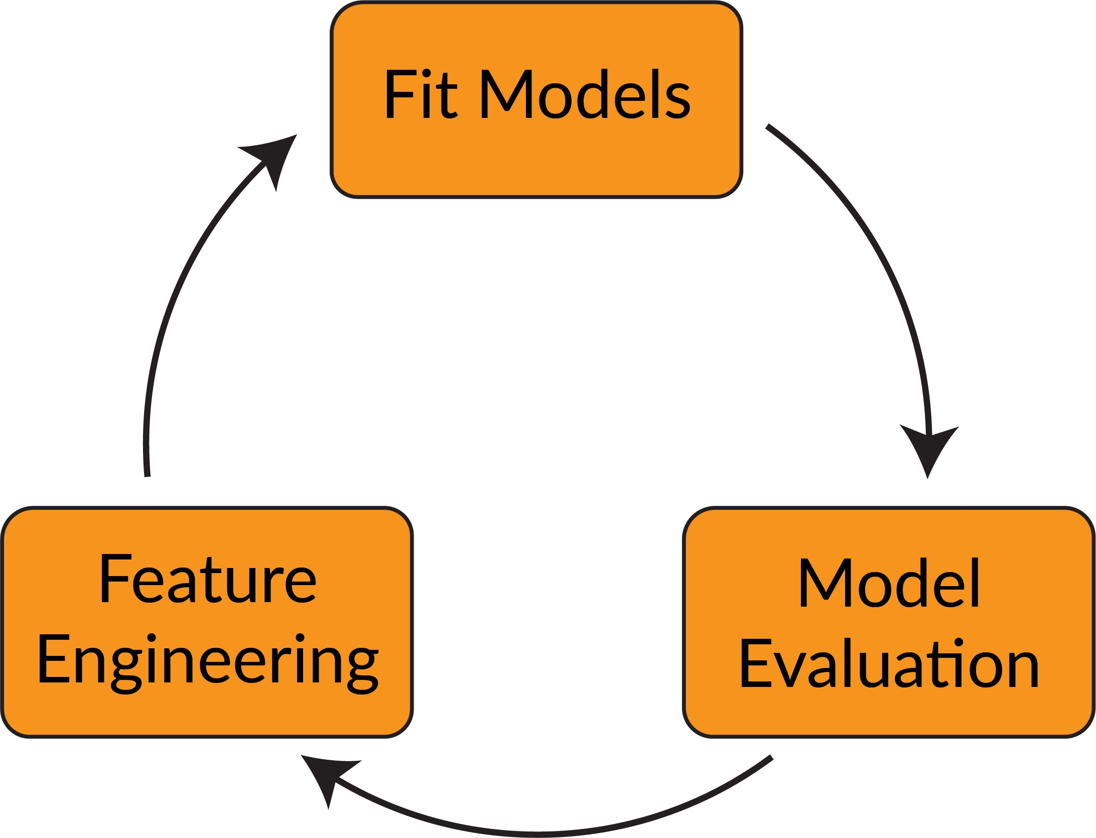
Figure 1.23: The life cycle of model creation
While this book is an introduction to deep learning with Keras, as mentioned earlier, we will start by utilizing scikit-learn. This will help us establish the fundamentals of building a machine learning model using the Python programming language.
Similar to scikit-learn, Keras makes it easy to create models in the Python programming language through an easy-to-use API. However, the goal of Keras is for the creation and training of neural networks, rather than machine learning models in general. ANNs represent a large class of machine learning algorithms, and they are so called because their architecture resembles the neurons in the human brain. The Keras library has many general-purpose functions built in, such as optimizers, activation functions, and layer properties, so that users, like in scikit-learn, do not have to code these algorithms from scratch.
scikit-learn was initially created in 2007 as a way to easily create machine learning models in the Python programming language by David Cournapeau. Since its inception, the library has grown immensely in popularity because of its ease of use, wide adoption within the machine learning community, and flexibility of use.
In the next section are a few of the advantages and disadvantages of using scikit-learn for machine learning purposes.
Advantages of scikit-learn are as follows:
Mature: scikit-learn is well established within the community and used by members of the community of all skill levels. The package includes most of the common machine learning algorithms for classification, regression, and clustering tasks.
User-friendly: scikit-learn features an easy-to-use API that enables beginners to efficiently prototype without having to have a deep understanding or code each specific mode.
Open source: There is an active open source community working to improve the library, add documentation, and release regular updates, which ensures that the package is stable and up to date.
Disadvantage of scikit-learn is as follows:
Neural network support lacking: Estimators with ANN algorithms are minimal.
The estimators in scikit-learn can generally be classified into supervised learning and unsupervised learning techniques. Supervised learning occurs when a target variable is present. A target variable is a variable of the dataset for which you are trying to predict given the other variables. Supervised learning requires the target variable to be known and models are trained in order to correctly predict this variable. Binary classification using logistic regression is a good example of a supervised learning technique.
In unsupervised learning, there is no target variable given in the training data, but models aim to assign a target variable. An example of an unsupervised learning technique is k-means clustering. This algorithm partitions data into a given number of clusters based on proximity to neighboring data points. The target variable assigned may be either the cluster number or cluster center.
An example of utilizing a clustering example in practice may look as follows. Imagine that you are a jacket manufacturer and your goal is to develop dimensions for various jacket sizes. You cannot create a custom-fit jacket for each customer, so one option you have to determine the dimensions for jackets is to sample the population of customers for various parameters that may be correlated to fit, such as height and weight. Then, you can group the population into clusters using scikit-learn's k-means clustering algorithm with a cluster number that matches with the number of jacket sizes you wish to produce. The cluster-centers that are created from the clustering algorithm become the parameters on which the jacket sizes are based. This is visualized in the following figure:
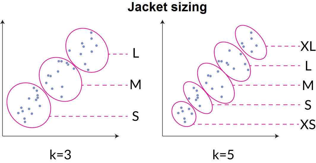
Figure 1.24: An unsupervised learning example of grouping customer parameters into clusters
There are even semi-supervised learning techniques in which unlabeled data is used in the training of machine learning models. This technique may be used if there is only a small amount of labeled data and a copious amount of unlabeled data. In practice, semi-supervised learning produces a significant improvement in model performance compared to unsupervised learning.
The scikit-learn library is ideal for beginners as the general concepts for building machine learning pipelines can be learned easily. Concepts such as data preprocessing, hyperparameter tuning, model evaluation, and many more are all included in the library. Even experienced users find the library easy to rapidly prototype models before using a more specialized machine learning library.
Indeed, the various machine learning techniques discussed such as supervised and unsupervised learning can be applied with Keras using neural networks with different architectures that will be discussed throughout the book.
Keras is designed to be a high-level neural network API that is built on top of frameworks such as TensorFlow, CNTK, or Theano. One of the great benefits of using Keras as an introduction to deep learning for beginners is that it is very user-friendly – advanced functions such as optimizers and layers are already built in to the library and do not have to be written from scratch. This is why Keras is popular not only amongst beginners, but also seasoned experts. Also, the library allows rapid prototyping of neural networks, supports a wide variety of network architectures, and can be run on both CPU and GPU.
Note
You can find the library and all documentation for Keras at the following link: https://Keras.io/.
Keras is used to create and train neural networks and does not offer much in terms of other machine learning algorithms, including supervised algorithms such as support vector machines and unsupervised algorithms such as k-means clustering. What Keras does offer, though, is a well-designed API to create and train neural networks, which takes away much of the effort required to apply linear algebra and multivariate calculus accurately.
The specific modules available from the Keras library, such as neural layers, cost functions, optimizers, initialization schemes, activation functions, and regularization schemes, will be explained thoroughly throughout the book. All these modules have relevant functions that can be used to optimize the performance for training neural networks for specific tasks.
Here are a few of the main advantages and disadvantages of using Keras for machine learning purposes:
User-friendly: Much like scikit-learn, Keras features an easy-to-use API that allows users to focus on model-building rather than the specifics of the algorithms.
Modular: The API consists of fully configurable modules that can all be plugged together and work seamlessly.
Extensible: It is relatively simple to add new modules to the library. This allows users to take advantage of the many robust modules within library while providing them the flexibility to create their own.
Open Source: Keras is an open source library and is constantly improving and adding modules to its code base thanks to the work of many collaborators working in conjunction to build improvements and help create a robust library for all.
Works with Python: Keras models are declared directly in Python rather than in separate configuration files, which allows Keras to take advantages of working with Python, such as ease of debugging and extensibility.
Advanced customization: While simple surface-level customization such as creating simple custom loss functions or neural layers is facile, it can be difficult to change how the underlying architecture works.
Lack of examples: Beginners often rely on examples to kick-start their learning. Advanced examples can be lacking in Keras documentation that can prevent beginners from advancing in their learning.
Keras offers those familiar with the Python programming language and machine learning the ability to create neural network architectures easily. Since neural networks are quite complicated, we will use scikit-learn to introduce many machine learning concepts before applying them out in the Keras library.
While machine learning libraries such as scikit-learn and Keras were created to help build and train predictive models, their practicality extends much further. One common use case of building models is that they can be utilized to perform predictions on new data. Once a model is trained, new observations can be fed into the model to generate predictions. Models may even be used as intermediate steps. For example, neural network models can be used as feature extractors, classifying objects in an image that can then be fed into a subsequent model, as illustrated in the following figure:
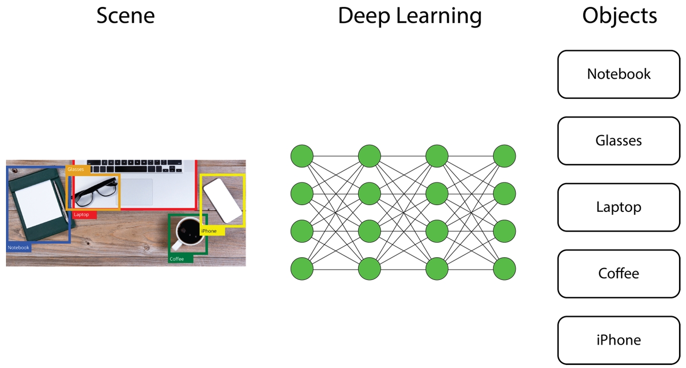
Figure 1.25: Classifying objects using deep learning
Another common use case for models is that they can be used to summarize datasets by learning representations of the data. Such models are known as auto-encoders, a type of neural network architecture that can be used to learn such representations of a given dataset. The dataset can thus be represented in a reduced dimension with minimal loss of information.
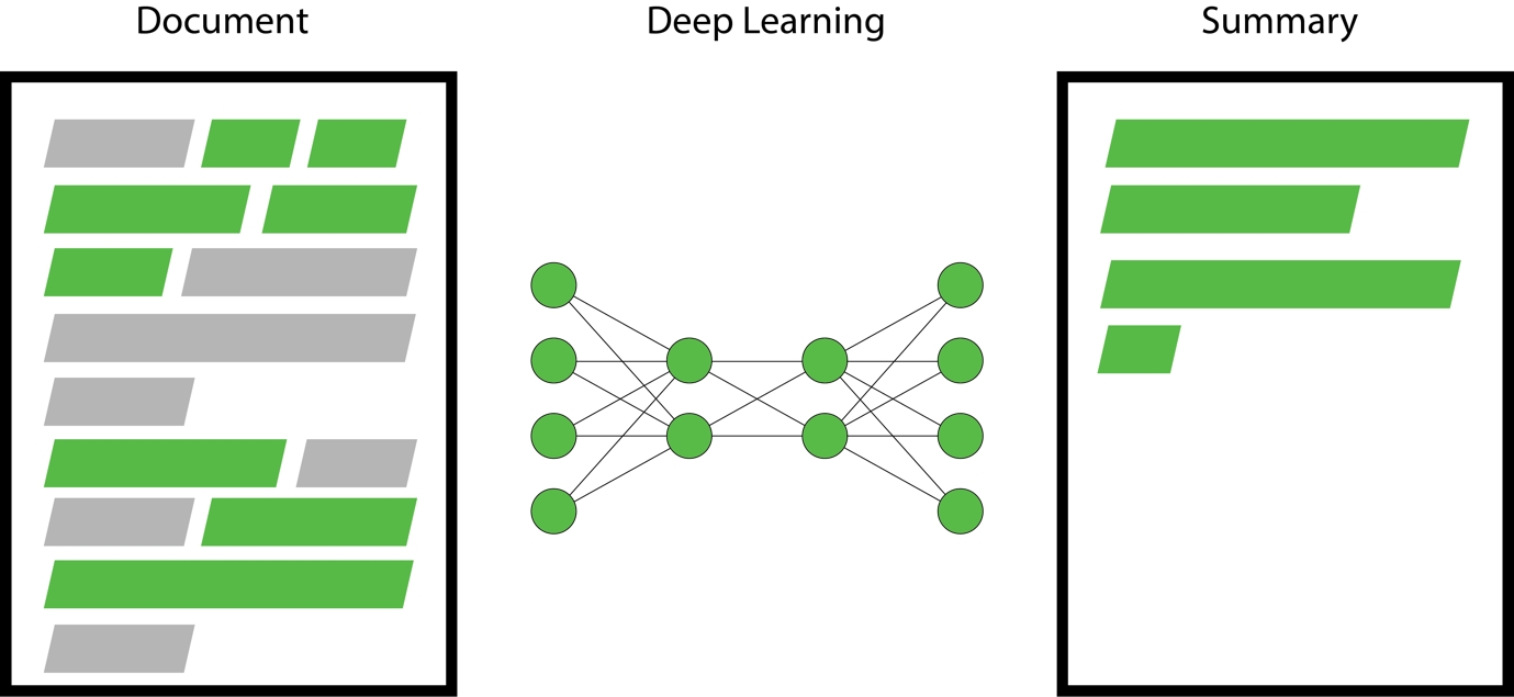
Figure 1.26: An example of using deep learning for text summarization
In this topic, we will begin fitting our model to the datasets that we have created. In this chapter, we will review the minimum steps required to create a machine learning model that can be applied to building models with any machine learning library, including scikit-learn and Keras.
This book is concerned with applications of deep learning. The vast majority of deep learning tasks are supervised learning, in which there is a given target, and we want to fit a model so that we can understand the relationship between the features and the target.
An example of supervised learning is identifying whether a picture contains a dog or a cat. We want to determine the relationship between the input (a matrix of pixel values) and the target variable, that is, whether the image is of a dog or a cat.
Figure 1.27: A simple supervised learning task to classify images into dogs and cats
Ofcourse, we may need many more images in our training dataset to robustly classify new images, but models that are trained on such a dataset are able to identify the various relationships that differentiate cats and dogs, which can then be used to predict labels for new data.
Supervised learning models are generally used for either classification or regression tasks.
The goal of classification tasks is to fit models from data with discrete categories that can be used to label unlabeled data. For example, these types of models can be used to classify images into dogs or cats. But it doesn't stop at binary classification; multi-label classification is also possible.
Most classification tasks output a probability for each unique class. The prediction is determined as the class with the highest probability, as can be seen in the following figure:
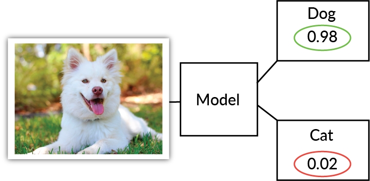
Figure 1.28: An illustration of a classification model labeling an image
Some of the most common classification algorithms are the following:
Logistic regression: This algorithm similar to linear regression, in which feature coefficients are learned and predictions are made by taking the sum of the product of the feature coefficients and features.
Decision trees: This algorithm follows a tree-like structure. Decisions are made at each node and branches represent possible options at the node, terminating in the predicted result.
ANNs: ANNs replicate the structure and performance of a biological neural network to perform pattern recognition tasks. An ANN consists of interconnected neurons, laid out with a set architecture, that pass information to each other until a result is achieved.
While the aim of classification tasks is to label datasets with discrete variables, the aim of regression tasks is to provide input data with continuous variables, and output a numerical value. For example, if you have a dataset of stock market prices, a classification task may predict whether to buy, sell, or hold, whereas a regression task will predict what the stock market price will be.
A simple, yet very popular, algorithm for regression tasks is linear regression. It consists of only one independent feature (x), whose relation with its dependent feature (y) is linear. Due to its simplicity, it is often overlooked, even though it performs very well for simple data problems.
Some of the most common classification algorithms are the following:
Linear regression: This algorithm learns feature coefficients and predictions are made by taking the sum of the product of the feature coefficients and features.
Support Vector Machines: This algorithm uses kernels to map input data into a multi-dimensional feature space to understand relationships between features and the target.
ANNs: ANNs replicate the structure and performance of a biological neural network to perform pattern recognition tasks. An ANN consists of interconnected neurons, laid out with a set architecture, that pass information to each other until a result is achieved.
Whenever we create machine learning models, we separate the data into training and test datasets. The training data is the set of data used to train the model. Typically, it is a large proportion, around 80%, of the total dataset. The test dataset is a sample of the dataset that is held out from the beginning and is used to provide an unbiased evaluation of the model. The test dataset should as accurately as possible represent real-world data. Any model evaluation metrics that are reported should be applied on the test dataset unless it's explicitly stated that the metrics have been evaluated on the training dataset. The reason for this is that models will typically perform better on the data they are trained on. Furthermore, models can overfit the training dataset, meaning that they perform well on the training dataset but perform poorly on the test dataset. A model is said to be overfitted to the data if the model performance is very good when evaluated on the training dataset, but performs poorly on the test dataset. Conversely, a model can be underfitted to the data. In this case, the model will fail to learn relationships between the features and the target, which will lead to poor performance when evaluated on both the training and test datasets. We aim for a balance of the two, not relying so heavily on the training dataset that we overfit, but allowing the model to learn the relationships between features and target so that the model generalizes well to new data. This concept is illustrated in the following figure:
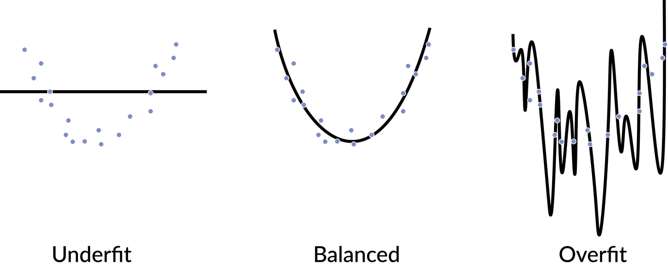
Figure 1.29: A example of under- and overfitting a dataset
There are many ways to split the dataset via sampling methods. One method to split a dataset into training is to simply randomly sample the data until you have the desired number of data points. This is often the default method in functions such as the scikit-learn train_test_spilt function. Another method is to stratify the sampling. In stratified sampling, each subpopulation is sampled independently. Each subpopulation is determined by the target variable. This can be advantageous in examples such as binary classification where the target variable is highly skewed toward one value or another, and random sampling may not provide data points of both values in the training and test datasets. There are also validation datasets, which we will address later in the chapter.
It is important to be able to evaluate our models effectively, not just in terms of the model's performance but also in the context of the problem we are trying to solve. For example, let's say we built a classification task to predict whether to buy, sell, or hold stock based on historical stock market prices. If our model only predicted to buy every time, this would not be a useful result because we may not have infinite resources to buy stocks. It may be better to be less accurate yet also include some sell predictions.
Common evaluation metrics for classification tasks are accuracy, precision, recall, and f1 score. Accuracy is defined as the number of correct predictions divided by the total number of predictions. Accuracy is very interpretable and relatable, and good for when there are balanced classes. When the classes are highly skewed, the accuracy can be misleading, however.
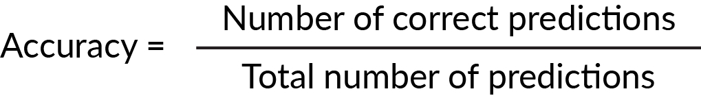
Figure 1.30: Formula to calculate accuracy
Precision is another useful metric. It's defined as the number of true positive results divided by the total number of positive results (true and false) predicted by the model.
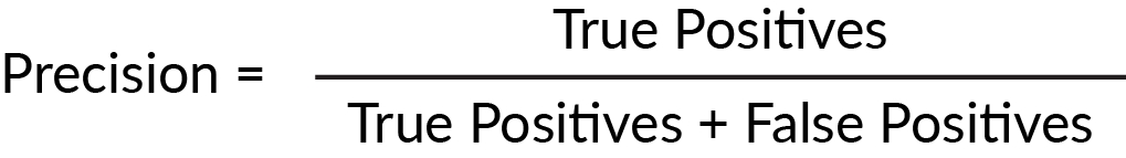
Figure 1.31: Formula to calculate precision
Recall is defined as the number of correct positive results divided by all positive results from the ground truth.

Figure 1.32: Formula to calculate recall
Both precision and recall are scored between zero and one, but scoring well on one may mean scoring poorly on the other. For example, a model may have high precision but low recall, which indicates that the model is very accurate but misses a large number of positive instances. It is useful to have a metric that combines recall and precision. Enter the f1 score, which determines how precise and robust your model is.
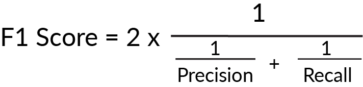
Figure 1.33: Formula to calculate f1 score
When evaluating models, it is helpful to look at a range of different evaluation metrics. They will help determine the most appropriate model and evaluate where the model is misclassifying predictions.
In this exercise, we will create a simple logistic regression model from the scikit-learn package. We will then create some model evaluation metrics and test the predictions against those model evaluation metrics.
We should always approach training any machine learning model training as an iterative approach, beginning first with a simple model, and using model evaluation metrics to evaluate the performance of the models. In this model, our goal is to classify the customers in the bank dataset into training and test datasets:
Load in the data:
import pandas as pd
feats = pd.read_csv('data/bank_data_feats_e3.csv', index_col=0)
target = pd.read_csv('data/bank_data_target_e2.csv', index_col=0)
We first begin by creating a test and train dataset. We will train the data using the training dataset and evaluate the performance of the model on the test dataset.
We will use test_size = 0.2, which means that 20% of the data will be reserved for testing, and we will set a number for the random_state parameter:
from sklearn.model_selection import train_test_split
test_size = 0.2
random_state = 42
X_train, X_test, y_train, y_test = train_test_split(feats, target, test_size=test_size, random_state=random_state)
We can print out the shape of each DataFrame to verify that the dimensions are correct:
print(f'Shape of X_train: {X_train.shape}')
print(f'Shape of y_train: {y_train.shape}')
print(f'Shape of X_test: {X_test.shape}')
print(f'Shape of y_test: {y_test.shape}')
The following figure shows the output of the preceding code:
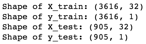
Figure 1.34: Shape of the test and training feature and target DataFrames
These dimensions look correct; each of the target datasets have a single column, the training feature and target DataFrames have the same number of rows, the same applies to the test feature and target DataFrames, and the test DataFrames are 20% of the total dataset.
Next, we have to instantiate our model:
from sklearn.linear_model import LogisticRegression
model = LogisticRegression(random_state=42)
While there are many arguments we can add to scikit-learn's logistic regression model, such as the type and value of regularization parameter, the type of solver, and the maximum number of iterations for the model to have, we will only pass random_state.
We then fit the model to the training data:
model.fit(X_train, y_train['y'])
To test the performance of the model, we compare the predictions of the model with the true values:
y_pred = model.predict(X_test)
There are many types of model evaluation metrics that we can use. Let's start with the accuracy, which is defined as the proportion of predicted values that equal the true values:
from sklearn import metrics
accuracy = metrics.accuracy_score(y_pred=y_pred, y_true=y_test)
print(f'Accuracy of the model is {accuracy*100:.4f}%')
The following figure shows the output of the preceding code:

Figure 1.35: Accuracy of the model
Other common evaluation metrics for classification models are the precision, recall, and f1 score. Scikit-learn has a function that can calculate all three, so we can use that:
precision, recall, fscore, _ = metrics.precision_recall_fscore_support(y_pred=y_pred, y_true=y_test, average='binary')
print(f'Precision: {precision:.4f}\nRecall: {recall:.4f}\nfscore: {fscore:.4f}')
Note
The underscore is used in Python for many reasons. It can be used to recall the value of the last expression in the interpreter, but in this case, we're using it to ignore specific values that are output by the function.
The following figure shows the output of the preceding code:
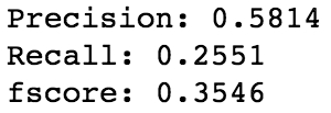
Figure 1.36: The other common evaluation metrics of the model
Since these metrics are scored between 0 and 1, the recall and fscore are not as impressive as the accuracy, though looking at all of these metrics together can help us to find where our models are doing well and where they could be improved by examining in which observations the model gets predictions incorrect.
We can also look at the coefficients that the model outputs to observe which features have a greater impact on the overall result of the prediction:
coef_list = [f'{feature}: {coef}' for coef, feature in sorted(zip(model.coef_[0], X_train.columns.values.tolist()))]
for item in coef_list:
    print(item)
The following figure shows the output of the preceding code:
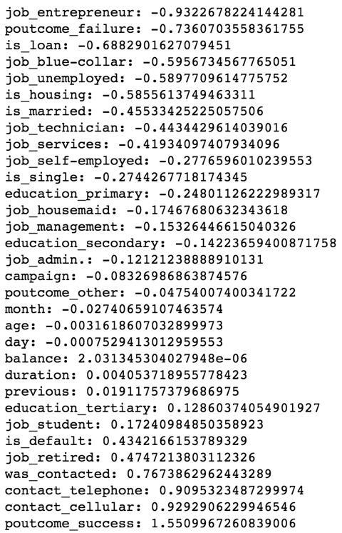
Figure 1.37: The sorted important features of the model with their respective coefficients
This activity has taught us how to create and train a predictive model to predict a target variable given feature variables. We split the feature and target dataset into training and test datasets. Then, we trained our model on the training dataset and evaluated our model on the test dataset. Finally, we observed the trained coefficients for this model.
In this topic, we will delve further into evaluating model performance and examine techniques of generalizing models to new data using regularization. Providing the context of a model's performance is extremely important. Our aim is to determine whether our model is performing well compared to trivial or obvious approaches. We do this by creating a baseline model against which machine learning models we train are compared. It is important to stress that all model evaluation metrics are evaluated and reported via the test dataset, since that will give us an understanding of how the model will perform on new data.
A baseline model should be a simple and well-understood procedure, and the performance of this model should be the lowest acceptable performance for any model we build. For classification models, a useful and easy baseline model is to calculate the mode outcome value. For example, in our example, if there are 60% false values, our baseline model would be to predict false for every value, which would give us an accuracy of 60%.
In this exercise, we will put model performance into context. The accuracy we attained from our model seemed good, but we need something to compare it to. Since machine learning model performance is relative, it is important to develop a robust baseline with which to compare models. We are again using the bank dataset, and our target variable is whether or not each customer subscribed to a product. Follow these steps to perform the exercise:
Import all the necessary dependencies and load in the target dataset:
import pandas as pd
target = pd.read_csv('data/bank_data_target_e2.csv', index_col=0)
Next, we have to calculate the relative proportion of each value of the target variables:
target['y'].value_counts()/target.shape[0]*100
The following figure shows the output of the preceding code:
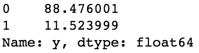
Figure 1.38: Relative proportion of each value
We can see in the dataset that 0 is represented 88.476% of the time – these are the customers that didn't subscribe to any product, and this is our baseline accuracy. Now for the other model evaluation metrics:
from sklearn import metrics
y_baseline = pd.Series(data=[0]*target.shape[0])
precision, recall, fscore, _ = metrics.precision_recall_fscore_support(y_pred=y_baseline, y_true=target['y'], average='macro')
Here, we've set the baseline model to predict 0 and have repeated the value to be the same as the number of rows in the test dataset.
Print the final output for precision, recall, and fscore:
print(f'Precision: {precision:.4f}\nRecall:{recall:.4f}\nfscore: {fscore:.4f}')The following figure shows the output of the preceding code:
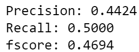
Figure 1.39: Final output values for precision, recall, and fscore
Now we have a baseline model that we can compare to our previous model, as well as any subsequent models. Now we can tell that while the accuracy of our previous model seemed high, it did not score much better than this baseline model.
We learned earlier in the chapter about overfitting and what it looks like. The hallmark of overfitting is when a model is trained to the training data and performs extremely well, yet performs terribly on test data. One reason for this could be that the model may be relying too heavily on certain features that lead to good performance in the training dataset but do not generalize well to new observations of data or the test dataset. One technique of avoiding this is called regularization. Regularization constrains the values of the coefficients toward zero, which discourages a complex model. There are many different types of regularization techniques. For example, in linear and logistic regression, ridge and lasso regularization are most common. In tree-based models, limiting the maximum depth of the trees acts as regularization.
There are two different types of regularization, namely L1 and L2. This term is either the L2 norm (the sum of the squared values) of the weights, or the L1 norm (the sum of the absolute values) of the weights. Since the l1 regularization parameter acts as a feature selector, it is able to reduce the coefficient of features to zero. We can use the output of this model to observe which features do not contribute much to the performance and remove them entirely if desired. The l2 regularization parameter will not reduce the coefficient of features to zero, so we will observe that they all have non-zero values.
The following code shows how to instantiate the models using these regularization techniques:
model_l1 = LogisticRegressionCV(Cs=Cs, penalty='l1', cv=10, solver='liblinear', random_state=42)
model_l2 = LogisticRegressionCV(Cs=Cs, penalty='l2', cv=10, random_state=42)
The following code shows how to fit the models:
model_l1.fit(X_train, y_train['y'])
model_l2.fit(X_train, y_train['y'])
The same concepts in lasso and ridge regularization can be applied to ANNs. However, the penalization occurs on the weight matrices rather than the coefficients. Dropout is another form of regularization that's used to prevent overfitting in ANNs. Dropout randomly selects nodes at each iteration and removes them, along with their connections:
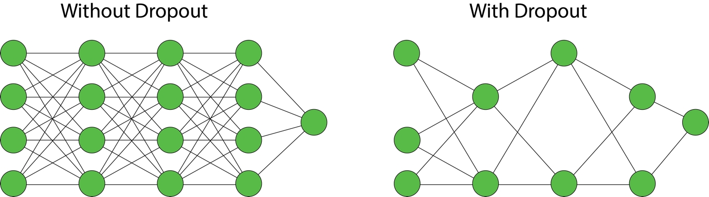
Figure 1.40: Dropout regularization in ANNs
Cross-validation is often used in conjunction with regularization to help tune hyperparameters. Take, for example, the penalization parameter in ridge and lasso regression, or the proportion of nodes to drop out at each iteration using the dropout technique with ANNs. How will you determine which parameter to use? One way is to run models for each value of the regularization parameter and evaluate on the test set; however, using the test set often can introduce bias into the model.
One popular example of cross-validation is called k-fold cross-validation. This technique gives us the ability to test our model on unseen data, while retaining a test set that we will use to test at the end. Using this method, the data is divided into k subsets. In each of the k iterations, k-1 of the subsets are used as training data and the remaining subset is used as a validation set. This is repeated k times until all k subsets have been used as validation sets. By using this technique, there is a significant reduction in bias, since most of the data is used for fitting. There is also a reduction in variation since most of the data is also used for validation. Typically, there are between 5 and 10 folds, and the technique can even be stratified, which is useful when there is a large imbalance of classes.
The following example shows 5-fold cross-validation with 20% held out as a test set. The remaining 80% is separated into 5 folds. 4 of those folds comprise the training data, and the remaining fold is the validation data. This repeated a total of 5 times until every fold has been used once as for validation.
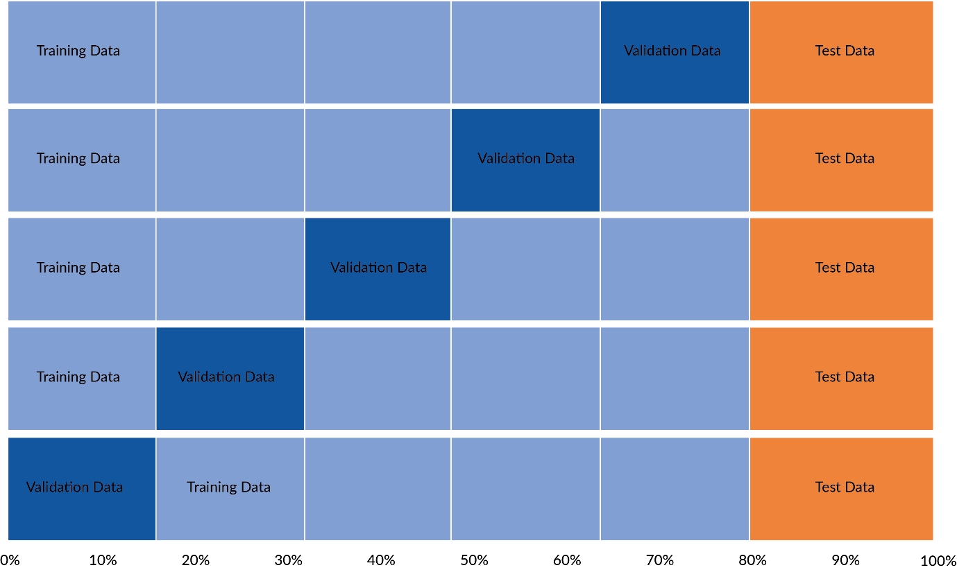
Figure 1.41: A figure demonstrating how 5-fold cross-validation works
In this activity, we will utilize the same logistic regression model from the scikit-learn package. This time, however, we will add regularization to the model and search for the optimum regularization parameter, a process often called hyperparameter tuning. After training the models, we will test the predictions and compare the model evaluation metrics to those produced by the baseline model and the model without regularization.
The steps we will take are as follows:
Load in the feature and target datasets of the bank dataset from 'data/bank_data_feats_e3.csv' and 'data/bank_data_target_e2.csv'.
Create training and testing datasets for each of the feature and target datasets. The training datasets will be used to train on, and the models will be evaluated using the test datasets.
Instantiate a model instance of the LogisticRegressionCV class of scikit-learn's linear_model package.
Fit the model to the training data.
Make predictions of the test dataset using the trained model.
Evaluate the models by comparing how they scored against the true values using the evaluation metrics.
In this chapter, we have covered how to prepare data and construct machine learning models. We have achieved this utilizing Python and libraries such as pandas and scikit-learn. We have also used the algorithms in scikit-learn to build our machine learning models.
In this chapter, we learned how to load data into Python, and how to manipulate data so that a machine learning model can be trained on the data. This involved converting all columns to numerical data types. We also learned to create a basic logistic regression classification model using scikit-learn algorithms. We divided the dataset into training and test datasets and fit the model to the training dataset. We evaluated the performance of the model on the test dataset using the model evaluation metrics: accuracy, precision, recall, and f1 score.
Finally, we iterated on this basic model by creating two models with different types of regularization to the model. We utilized cross-validation to determine the optimal parameter to use for the regularization parameter.
In the next chapter, we will use the same concept learned in this chapter; however, we will create the model using the Keras library. We will use the same dataset, and attempt to predict the same target value, for the same classification task. We will cover how to use regularization, cross-validation, and model evaluation metrics when fitting our neural network to the data.