Download code from GitHub
"The way Moore's Law occurs in computing is really unprecedented in other walks of life. If the Boeing 747 obeyed Moore's Law, it would travel a million miles an hour, it would be shrunken down in size, and a trip to New York would cost about five dollars. Those enormous changes just aren't part of our everyday experience."
— Nathan Myhrvold, former Chief Technology Officer at Microsoft, 1995
The way Moore's Law has benefitted QlikView is really unprecedented amongst other BI systems.
QlikView began life in 1993 in Lund, Sweden. Originally titled "QuickView", they had to change things when they couldn't obtain a copyright on that name, and thus "QlikView" was born.
After years of steady growth, something really good happened for QlikView around 2005/2006—the Intel x64 processors became the dominant processors in Windows servers. QlikView had, for a few years, supported the Itanium version of Windows; however, Itanium never became a dominant server processor. Intel and AMD started shipping the x64 processors in 2004 and, by 2006, most servers sold came with an x64 processor—whether the customer wanted 64-bit or not. Because the x64 processors could support either x86 or x64 versions of Windows, the customer didn't even have to know. Even those customers who purchased the x64 version of Windows 2003 didn't really know this because all of their x86 software would run just as well (perhaps with a few tweaks).
But x64 Windows was fantastic for QlikView! Any x86 process is limited to a maximum of 2 GB of physical memory. While 2 GB is quite a lot of memory, it wasn't enough to hold the volume of data that a true enterprise-class BI tool needed to handle. In fact, up until version 9 of QlikView, there was an in-built limitation of about 2 billion rows (actually, 2 to the power of 31) in the number of records that QlikView could load. On x86 processors, QlikView was really confined to the desktop.
x64 was a very different story. Early Intel implementations of x64 could address up to 64 GB of memory. More recent implementations allow up to 256 TB, although Windows Server 2012 can only address 4 TB. Memory is suddenly less of an obstacle to enterprise data volumes.
The other change that happened with processors was the introduction of multi-core architecture. At the time, it was common for a high-end server to come with 2 or 4 processors. Manufacturers came up with a method of putting multiple processors, or cores, on one physical processor. Nowadays, it is not unusual to see a server with 32 cores. High-end servers can have many, many more.
One of QlikView's design features that benefitted from this was that their calculation engine is multithreaded. That means that many of QlikView's calculations will execute across all available processor cores. Unlike many other applications, if you add more cores to your QlikView server, you will, in general, add more performance.
So, when it comes to looking at performance and scalability, very often, the first thing that people look at to improve things is to replace the hardware. This is valid of course! QlikView will almost always work better with newer, faster hardware. But before you go ripping out your racks, you should have a good idea of exactly what is going on with QlikView. Knowledge is power; it will help you tune your implementation to make the best use of the hardware that you already have in place.
The following are the topics we'll be covering in this chapter:
Reviewing basic performance tuning techniques
Generating test data
Understanding how QlikView stores its data
Looking at strategies to reduce the data size and to improve performance
Using Direct Discovery
Testing scalability with JMeter
There are many ways in which you may have learned to develop with QlikView. Some of them may have talked about performance and some may not have. Typically, you start to think about performance at a later stage when users start complaining about slow results from a QlikView application or when your QlikView server is regularly crashing because your applications are too big.
In this section, we are going to quickly review some basic performance tuning techniques that you should, hopefully, already be aware of. Then, we will start looking at how we can advance your knowledge to master level.
Removing unneeded data might seem easy in theory, but sometimes it is not so easy to implement—especially when you need to negotiate with the business. However, the quickest way to improve the performance of a QlikView application is to remove data from it. If you can reduce your number of fact rows by half, you will vastly improve performance. The different options are discussed in the next sections.
The first option is to simply reduce the number of rows. Here we are interested in Fact or Transaction table rows—the largest tables in your data model. Reducing the number of dimension table rows rarely produces a significant performance improvement.
The easiest way to reduce the number of these rows is usually to limit the table by a value such as the date. It is always valuable to ask the question, "Do we really need all the transactions for the last 10 years?" If you can reduce this, say to 2 years, then the performance will improve significantly.
We can also choose to rethink the grain of the data—to what level of detail we hold the information. By aggregating the data to a higher level, we will often vastly reduce the number of rows.
The second option is to reduce the width of tables—again, especially Fact or Transaction tables. This means looking at fields that might be in your data model but do not actually get used in the application. One excellent way of establishing this is to use the Document Analyzer tool by Rob Wunderlich to examine your application (http://robwunderlich.com/downloads).
As well as other excellent uses, Rob's tool looks at multiple areas of an application to establish whether fields are being used or not. It will give you an option to view fields that are not in use and has a useful DROP FIELD Statements listbox from which you can copy the possible values. The following screenshot shows an example (from the default document downloadable from Rob's website):
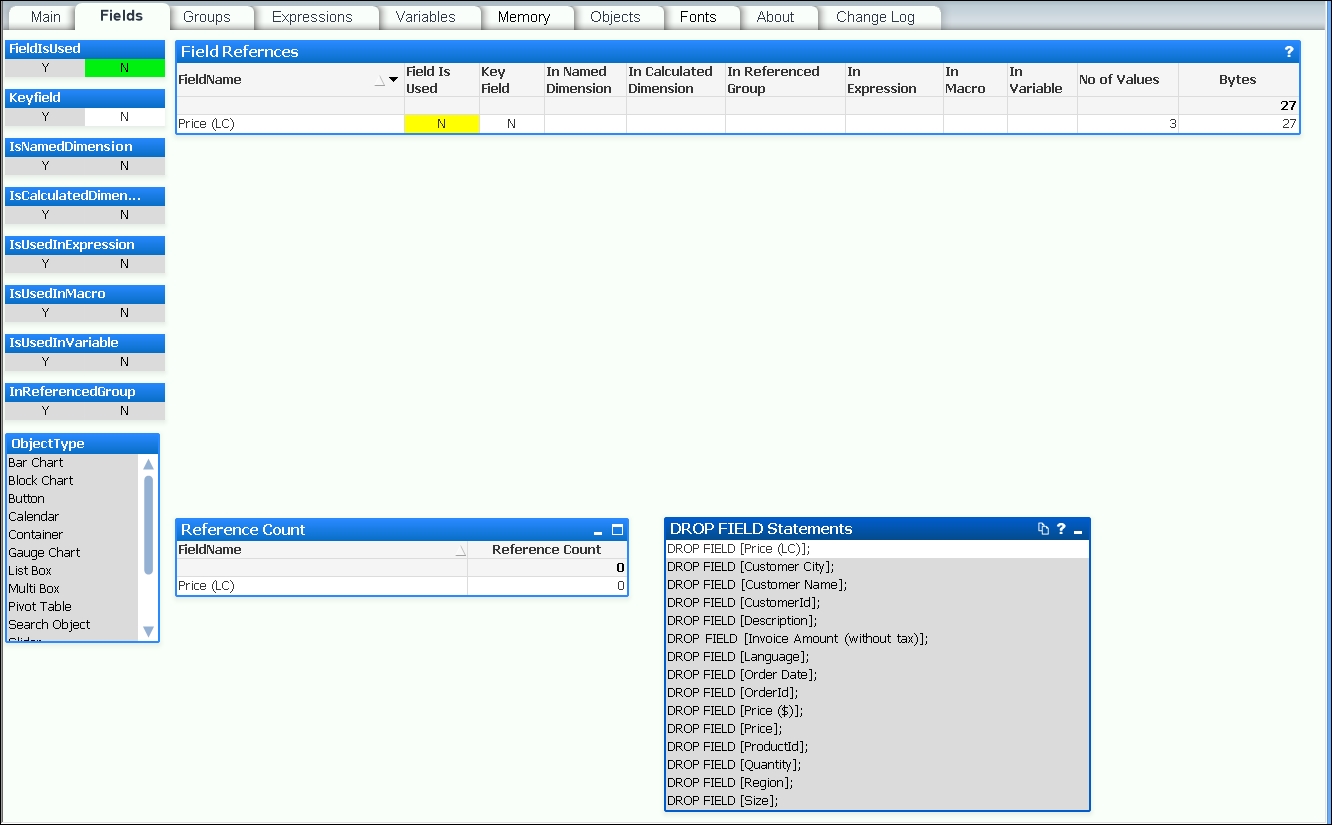
Adding these DROP FIELD statements into the end of a script makes it very easy to remove fields from your data model without having to dive into the middle of the script and try to remove them during the load—which could be painful.
There is a potential issue here; if you have users using collaboration objects—creating their own charts—then this tool will not detect that usage. However, if you use the DROP FIELD option, then it is straightforward to add a field back if a user complains that one of their charts is not working.
Of course, the best practice would be to take the pain and remove the fields from the script by either commenting them out or removing them completely from their load statements. This is more work, because you may break things and have to do additional debugging, but it will result in a better performing script.
Often, you will have a text value in a key field, for example, something like an account number that has alphanumeric characters. These are actually quite poor for performance compared to an integer value and should be replaced with numeric keys.
Note
There is some debate here about whether this makes a difference at all, but the effect is to do with the way the data is stored under the hood, which we will explore later. Generated numeric keys are stored slightly differently than text keys, which makes things work better.
The strategy is to leave the text value (account number) in the dimension table for use in display (if you need it!) and then use the AutoNumber function to generate a numeric value—also called a surrogate key—to associate the two tables.
For example, replace the following:
Account:
Load
   AccountId,
   AccountName,
   …
From Account.qvd (QVD);

Transaction:
Load
   TransactionId,
   AccountId,
   TransactionDate,
   …
From Transaction.qvd (QVD);
With the following:
Account:
Load
   AccountId,
   AutoNumber(AccountId) As Join_Account,
   AccountName,
   …
From Account.qvd (QVD);

Transaction:
Load
   TransactionId,
   AutoNumber(AccountId) As Join_Account,
   TransactionDate,
   …
From Transaction.qvd (QVD);
The AccountId field still exists in the Account table for display purposes, but the association is on the new numeric field, Join_Account.
We will see later that there is some more subtlety to this that we need to be aware of.
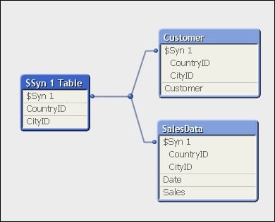
A synthetic key, caused when tables are associated on two or more fields, actually results in a whole new data table of keys within the QlikView data model.
The following screenshot shows an example of a synthetic key using Internal Table View within Table Viewer in QlikView:
In general, it is recommended to remove synthetic keys from your data model by generating your own keys (for example, using AutoNumber):
Load
   AutoNumber(CountryID & '-' & CityID) As ClientID,
   Date,
   Sales
From Fact.qvd (qvd);
The following screenshot shows the same model with the synthetic key resolved using the AutoNumber method:
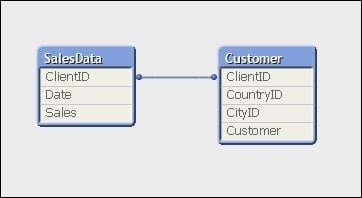
This removes additional data in the data tables (we'll cover more on this later in the chapter) and reduces the number of tables that queries have to traverse.
It is enormously useful to be able to quickly generate test data so that we can create QlikView applications and test different aspects of development and discover how different development methods work. By creating our own set of data, we can abstract problems away from the business issues that we are trying to solve because the data is not connected to those problems. Instead, we can resolve the technical issue underlying the business issue. Once we have resolved that issue, we will have built an understanding that allows us to more quickly resolve the real problems with the business data.
We might contemplate that if we are developers who only have access to a certain dataset, then we will only learn to solve the issues in that dataset. For true mastery, we need to be able to solve issues in many different scenarios, and the only way that we can do that is to generate our own test data to do that with.
Dimension tables will generally have lower numbers of records; there are a number of websites online that will generate this type of data for you.
The following screenshot demonstrates setting up a Customer extract in Mockaroo:

This allows us to create 1,000 customer records that we can include in our QlikView data model. The extract is in the CSV format, so it is quite straightforward to load into QlikView.
While we might often abdicate the creation of test dimension tables to a third-party website like this, we should always try and generate the Fact table data ourselves.
A good way to do this is to simply generate rows with a combination of the AutoGenerate() and Rand() functions.
For even more advanced use cases, we can look at using statistical functions such as NORMINV to generate normal distributions. There is a good article on this written by Henric Cronström on Qlik Design Blog at http://community.qlik.com/blogs/qlikviewdesignblog/2013/08/26/monte-carlo-methods.
We should be aware of the AutoGenerate() function that will just simply generate empty rows of data. We can also use the Rand() function to generate a random number between 0 and 1 (it works both in charts and in the script). We can then multiply this value by another number to get various ranges of values.
In the following example, we load a previously generated set of dimension tables—Customer, Product, and Employee. We then generate a number of order header and line rows based on these dimensions, using random dates in a specified range.
First, we will load the Product table and derive a couple of mapping tables:
// Load my auto generated dimension files
Product:
LOAD ProductID,
     Product,
     CategoryID,
     SupplierID,
     Money#(CostPrice, '$#,##0.00', '.', ',') As CostPrice,
     Money#(SalesPrice, '$#,##0.00', '.', ',') As SalesPrice
FROM
Products.txt
(txt, utf8, embedded labels, delimiter is '\t', msq);


Product_Cost_Map:
Mapping Load
   ProductID,
   Num(CostPrice)
Resident Product;

Product_Price_Map:
Mapping Load
   ProductID,
   Num(SalesPrice)
Resident Product;
Now load the other dimension tables:
Customer:
LOAD CustomerID,
     Customer,
     City,
     Country,
     Region,
     Longitude,
     Latitude,
     Geocoordinates
FROM
Customers.txt
(txt, codepage is 1252, embedded labels, delimiter is '\t', msq);

Employee:
LOAD EmployeeID,
     Employee,
     Grade,
     SalesUnit
FROM
Employees.txt
(txt, codepage is 1252, embedded labels, delimiter is '\t', msq)
Where Match(Grade, 0, 1, 2, 3);  // Sales people
We will store the record counts from each table in variables:
// Count the ID records in each table
Let vCustCount=FieldValueCount('CustomerID');
Let vProdCount=FieldValueCount('ProductID');
Let vEmpCount=FieldValueCount('EmployeeID');
We now generate some date ranges to use in the data calculation algorithm:
// Work out the days
Let vStartYear=2009;      // Arbitrary - change if wanted
Let vEndYear=Year(Now()); // Generate up to date data
// Starting the date in April to allow
// offset year testing
Let vStartDate=Floor(MakeDate($(vStartYear),4,1));
Let vEndDate=Floor(MakeDate($(vEndYear),3,31));
Let vNumDays=vEndDate-vStartDate+1;
Note
Downloading the example code
You can download the example code files from your account at http://www.packtpub.com for all the Packt Publishing books you have purchased. If you purchased this book elsewhere, you can visit http://www.packtpub.com/support and register to have the files e-mailed directly to you.
Run a number of iterations to generate data. By editing the number of iterations, we can increase or decrease the amount of data generated:
// Create a loop of 10000 iterations
For i=1 to 10000

   // "A" type records are for any date/time

   // Grab a random employee and customer
   Let vRnd = Floor(Rand() * $(vEmpCount));
   Let vEID = Peek('EmployeeID', $(vRnd), 'Employee');
   Let vRnd = Floor(Rand() * $(vCustCount));
   Let vCID = Peek('CustomerID', $(vRnd), 'Customer');

   // Create a date for any Time of Day  9-5
   Let vOrderDate = $(vStartDate) + Floor(Rand() * $(vNumDays)) + ((9/24) + (Rand()/3));

   // Calculate a random freight amount
   Let vFreight = Round(Rand() * 100, 0.01);

   // Create the header record
   OrderHeader:
   Load
      'A' & $(i)       As OrderID,
      $(vOrderDate)    As OrderDate,
      $(vCID)       As CustomerID,
      $(vEID)       As EmployeeID,
      $(vFreight)    As Freight
   AutoGenerate(1);

   // Generate Order Lines

   // This factor allows us to generate a different number of
   // lines depending on the day of the week
   Let vWeekDay = Num(WeekDay($(vOrderDate)));
   Let vDateFactor = Pow(2,$(vWeekDay))*(1-(Year(Now())-Year($(vOrderDate)))*0.05);

   // Calculate the random number of lines
   Let vPCount = Floor(Rand() * $(vDateFactor)) + 1;

   For L=1 to $(vPCount)
      // Calculate random values
      Let vQty = Floor(Rand() * (50+$(vDateFactor))) + 1;
      Let vRnd = Floor(Rand() * $(vProdCount));
      Let vPID = Peek('ProductID', $(vRnd), 'Product');
      Let vCost = ApplyMap('Product_Cost_Map', $(vPID), 1);
      Let vPrice = ApplyMap('Product_Price_Map', $(vPID), 1);

      OrderLine:
      Load
         'A' & $(i)       As OrderID,
         $(L)         As LineNo,
         $(vPID)         As ProductID,
         $(vQty)         As Quantity,
         $(vPrice)      As SalesPrice,
         $(vCost)      As SalesCost,
         $(vQty)*$(vPrice) As LineValue,
         $(vQty)*$(vCost) As LineCost
      AutoGenerate(1);

   Next

   // "B" type records are for summer peak

   // Summer Peak - Generate additional records for summer
   // months to simulate a peak trading period
   Let vY = Year($(vOrderDate));
   Let vM = Floor(Rand()*2)+7;
   Let vD = Day($(vOrderDate));
   Let vOrderDate = Floor(MakeDate($(vY),$(vM),$(vD))) + ((9/24) + (Rand()/3));

   if Rand() > 0.8 Then

      // Grab a random employee and customer
      Let vRnd = Floor(Rand() * $(vEmpCount));
      Let vEID = Peek('EmployeeID', $(vRnd), 'Employee');
      Let vRnd = Floor(Rand() * $(vCustCount));
      Let vCID = Peek('CustomerID', $(vRnd), 'Customer');

      // Calculate a random freight amount
      Let vFreight = Round(Rand() * 100, 0.01);
      // Create the header record
      OrderHeader:
      Load
         'B' & $(i)       As OrderID,
         $(vOrderDate)    As OrderDate,
         $(vCID)       As CustomerID,
         $(vEID)       As EmployeeID,
         $(vFreight)    As Freight
      AutoGenerate(1);

      // Generate Order Lines

      // This factor allows us to generate a different number of
      // lines depending on the day of the week
      Let vWeekDay = Num(WeekDay($(vOrderDate)));
      Let vDateFactor = Pow(2,$(vWeekDay))*(1-(Year(Now())-Year($(vOrderDate)))*0.05);

      // Calculate the random number of lines
      Let vPCount = Floor(Rand() * $(vDateFactor)) + 1;

      For L=1 to $(vPCount)

         // Calculate random values
         Let vQty = Floor(Rand() * (50+$(vDateFactor))) + 1;
         Let vRnd = Floor(Rand() * $(vProdCount));
         Let vPID = Peek('ProductID', $(vRnd), 'Product');
         Let vCost = ApplyMap('Product_Cost_Map', $(vPID), 1);
         Let vPrice = ApplyMap('Product_Price_Map', $(vPID), 1);

         OrderLine:
         Load
            'B' & $(i)       As OrderID,
            $(L)         As LineNo,
            $(vPID)         As ProductID,
            $(vQty)         As Quantity,
            $(vPrice)      As SalesPrice,
            $(vCost)      As SalesCost,
            $(vQty)*$(vPrice) As LineValue,
            $(vQty)*$(vCost) As LineCost
         AutoGenerate(1);
      Next

   End if
Next

// Store the Generated Data to QVD
Store OrderHeader into OrderHeader.qvd;
Store OrderLine into OrderLine.qvd;QlikView is really good at storing data. It operates on data in memory, so being able to store a lot of data in a relatively small amount of memory gives the product a great advantage—especially as Moore's Law continues to give us bigger and bigger servers.
Understanding how QlikView stores its data is fundamental in mastering QlikView development. Writing load script with this understanding will allow you to load data in the most efficient way so that you can create the best performing applications. Your users will love you.
A great primer on how QlikView stores its data is available on Qlik Design Blog, written by Henric Cronström (http://community.qlik.com/blogs/qlikviewdesignblog/2012/11/20/symbol-tables-and-bit-stuffed-pointers).
From a simple level, consider the following small table:
|
First name |
Surname |
Country |
|---|---|---|
|
John |
Smith |
USA |
|
Jane |
Smith |
USA |
|
John |
Doe |
Canada |
For the preceding table, QlikView will create three symbol tables like the following:
|
Index |
Value |
|---|---|
|
1010 |
John |
|
1011 |
Jane |
|
Index |
Value |
|---|---|
|
1110 |
Smith |
|
1111 |
Doe |
|
Index |
Value |
|---|---|
|
110 |
USA |
|
111 |
Canada |
And the data table will look like the following:
|
First name |
Surname |
Country |
|---|---|---|
|
1010 |
1110 |
110 |
|
1011 |
1110 |
110 |
|
1010 |
1111 |
111 |
This set of tables will take up less space than the original data table for the following three reasons:
The binary indexes are bit-stuffed in the data table—they only take up as much space as needed.
The binary index, even though repeated, will take up less space than the text values. The Unicode text just for "USA" takes up several bytes—the binary index takes less space than that.
Each, larger, text value is only stored once in the symbol tables.
So, to summarize, each field in the data model will be stored in a symbol table (unless, as we will see later, it is a sequential integer value) that contains the unique values and an index value. Every table that you create in the script—including any synthetic key tables—will be represented as a data table containing just the index pointers.
To help us understand what is going on in a particular QlikView document, we can export details about where all the memory is being used. This export file will tell us how much memory is being used by each field in the symbol tables, the data tables, chart objects, and so on.
Perform the following steps to export the memory statistics for a document:
To export the memory statistics, you need to open Document Properties from the Settings menu (Ctrl + Alt + D). On the General tab, click on the Memory Statistics button, as shown in the following screenshot:

After you click on the button, you will be prompted to enter file information. Once you have entered the path and filename, the file will be exported. It is a tab-delimited data file:

The easiest way to analyze this file is to import it into a new QlikView document:

We can now see exactly how much space our data is taking up in the symbol tables and in the data tables. We can also look at chart calculation performance to see whether there are long running calculations that we need to tune. Analyzing this data will allow us to make valuable decisions about where we can improve performance in our QlikView document.
One thing that we need to be cognizant of is that the memory usage and calculation time of charts will only be available if that chart has actually been opened. The calculation time of the charts may also not be accurate as it will usually only be correct if the chart has just been opened for the first time—subsequent openings and changes of selection will most probably be calculated from the cache, and a cache execution should execute a lot quicker than a non-cached execution. Other objects may also use similar expressions, and these will therefore already be cached. We can turn the cache off—although only for testing purposes, as it can really kill performance.
Using some of the test data that we have generated, or any other data that you might want, we can discover more about how QlikView handles different scenarios. Understanding these different situations will give you real mastery over data load optimization.
To begin with, let's see what happens when we load two largish tables that are connected by a key. So, let's ignore the dimension tables and load the order data using a script like the following:
Order:
LOAD OrderID,
OrderDate,
CustomerID,
EmployeeID,
Freight
FROM
[..\Scripts\OrderHeader.qvd]
(qvd);
OrderLine:
LOAD OrderID,
LineNo,
ProductID,
Quantity,
SalesPrice,
SalesCost,
LineValue,
LineCost
FROM
[..\Scripts\OrderLine.qvd]
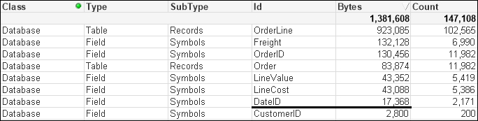
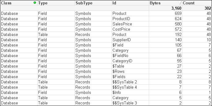
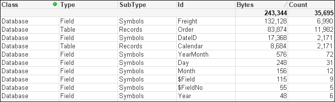
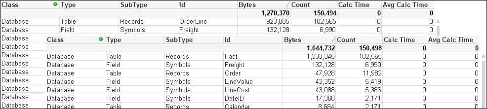
(qvd);The preceding script will result in a database memory profile that looks like the following. In the following screenshot, Database has been selected for Class:
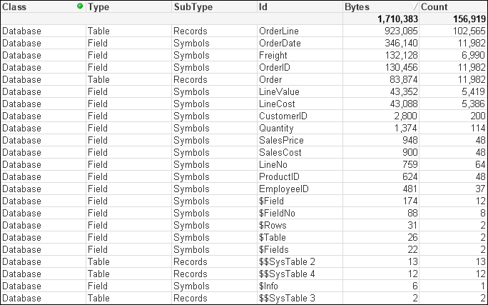
There are some interesting readings in this table. For example, we can see that when the main data table—OrderLine—is stored with just its pointer records, it takes up just 923,085 bytes for 102,565 records. That is an average of only 9 bytes per record. This shows the space benefit of the bit-stuffed pointer mechanism as described in Henric's blog post.
The largest individual symbol table is the OrderDate field. This is very typical of a TimeStamp field, which will often be highly unique, have long decimal values, and have the Dual text value, and so often takes up a lot of memory—28 bytes per value.
The number part of a TimeStamp field contains an integer representing the date (number of days since 30th December 1899) and a decimal representing the time. So, let's see what happens with this field if we turn it into just an integer—a common strategy with these fields as the time portion may not be important:
Order:
LOAD OrderID,
Floor(OrderDate) As DateID,
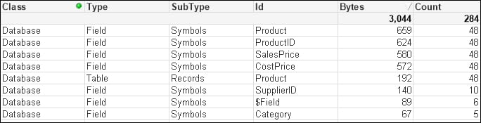
...This changes things considerably:
The number of unique values has been vastly reduced, because the highly unique date and time values have been replaced with a much lower cardinality (2171) date integer, and the amount of memory consumed is also vastly reduced as the integer values are only taking 8 bytes instead of the 28 being taken by each value of the TimeStamp field.
The next field that we will pay attention to is OrderID. This is the key field, and key fields are always worth examining to see whether they can be improved. In our test data, the OrderID field is alphanumeric—this is not uncommon for such data. Alphanumeric data will tend to take up more space than numeric data, so it is a good idea to convert it to integers using the AutoNumber function.
AutoNumber accepts a text value and will return a sequential integer. If you pass the same text value, it will return the same integer. This is a great way of transforming alphanumeric ID values into integers. The code will look like the following:
Order:
LOAD AutoNumber(OrderID) As OrderID,
     Floor(OrderDate) As DateID,
   ...

OrderLine:
LOAD AutoNumber(OrderID) As OrderID,
     LineNo,
   ...
This will result in a memory profile like the following:
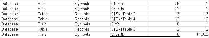
The OrderID field is now showing as having 0 bytes! This is quite interesting because what QlikView does with a field containing sequential integers is that it does not bother to store the value in the symbol table at all; it just uses the value as the pointer in the data table. This is a great design feature and gives us a good strategy for reducing data sizes.
We could do the same thing with the CustomerID and EmployeeID fields:
Order:
LOAD AutoNumber(OrderID) As OrderID,
     Floor(OrderDate) As DateID,
     AutoNumber(CustomerID) As CustomerID,
     AutoNumber(EmployeeID) As EmployeeID,
     ...
That has a very interesting effect on the memory profile:
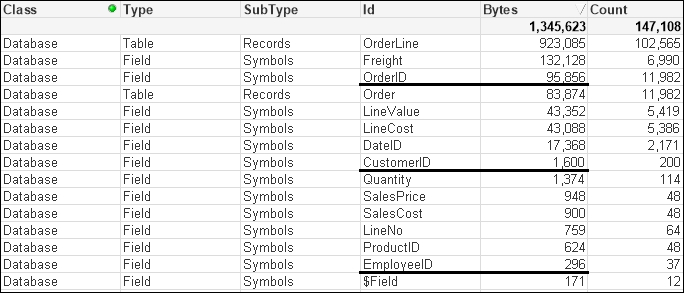
Our OrderID field is now back in the Symbols table. The other two tables are still there too. So what has gone wrong?
Because we have simply used the AutoNumber function across each field, now none of them are perfectly sequential integers and so do not benefit from the design feature. But we can do something about this because the AutoNumber function accepts a second parameter—an ID—to identify different ranges of counters. So, we can rejig the script in the following manner:
Order:
LOAD AutoNumber(OrderID, 'Order') As OrderID,
     Floor(OrderDate) As DateID,
     AutoNumber(CustomerID, 'Customer') As CustomerID,
     AutoNumber(EmployeeID, 'Employee') As EmployeeID,
     ...

OrderLine:
LOAD AutoNumber(OrderID, 'Order') As OrderID,
     LineNo,
     ...
This should give us the following result:
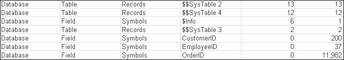
This is something that you should consider for all key values, especially from a modeling best practice point of view. There are instances when you want to retain the ID value for display or search purposes. In that case, a copy of the value should be kept as a field in a dimension table and the AutoNumber function used on the key value.
Note
It is worth noting that it is often good to be able to see the key associations—or lack of associations—between two tables, especially when troubleshooting data issues. Because AutoNumber obfuscates the values, it makes that debugging a bit harder. Therefore, it can be a good idea to leave the application of AutoNumber until later on in the development cycle, when you are more certain of the data sources.
For this example, we will use some of the associated dimension tables—Category and Product. These are loaded in the following manner:
Category:
LOAD CategoryID,
     Category
FROM
[..\Scripts\Categories.txt]
(txt, codepage is 1252, embedded labels, delimiter is '\t', msq);

Product:
LOAD ProductID,
     Product,
     CategoryID,
     SupplierID,
     CostPrice,
     SalesPrice
FROM
[..\Scripts\Products.txt]
(txt, codepage is 1252, embedded labels, delimiter is '\t', msq);
This has a small memory profile:
The best way to improve the performance of these tables is to remove the CategoryID field by moving the Category value into the Product table. When we have small lookup tables like this, we should always consider using ApplyMap:
Category_Map:
Mapping
LOAD CategoryID,
     Category
FROM
[..\Scripts\Categories.txt]
(txt, codepage is 1252, embedded labels, delimiter is '\t', msq);

Product:
LOAD ProductID,
     Product,
     //CategoryID,
     ApplyMap('Category_Map', CategoryID, 'Other') As Category,
     SupplierID,
     CostPrice,
     SalesPrice
FROM
[..\Scripts\Products.txt]
(txt, codepage is 1252, embedded labels, delimiter is '\t', msq);
By removing the Symbols table and the entry in the data table, we have reduced the amount of memory used. More importantly, we have reduced the number of joins required to answer queries based on the Category table:
If the associated dimension table has more than two fields, it can still have its data moved into the primary dimension table by loading multiple mapping tables; this is useful if there is a possibility of many-to-many joins. You do have to consider, however, that this does make the script a little more complicated and, in many circumstances, it is a better idea to simply join the tables.
For example, suppose that we have the previously mentioned Product table and an associated Supplier table that is 3,643 bytes:
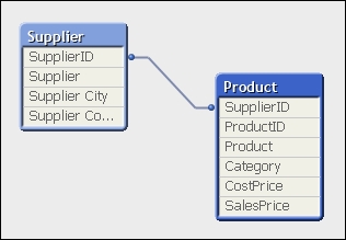
By joining the Supplier table to the Product table and then dropping SupplierID, we might reduce this down to, say, 3,499 bytes, but more importantly, we improve the query performance:
Join (Product)
LOAD SupplierID,
     Company As Supplier,
     ...

Drop Field SupplierID;Joining tables together is not always the best approach from a memory point of view. It could be possible to attempt to create the ultimate joined table model of just having one table containing all values. This will work, and query performance should, in theory, be quite fast. However, the way QlikView works is the wider and longer the table you create, the wider and longer the underlying pointer data table will be. Let's consider an example.
Quite often, there will be a number of associated fields in a fact table that have a lower cardinality (smaller number of distinct values) than the main keys in the fact table. A quite common example is having date parts within the fact table. In that case, it can actually be a good idea to remove these values from the fact table and link them via a shared key. So, for example, consider we have an Order table loaded in the following manner:
Order:
LOAD AutoNumber(OrderID, 'Order') As OrderID,
     Floor(OrderDate) As DateID,
     Year(OrderDate) As Year,
     Month(OrderDate) As Month,
     Day(OrderDate) As Day,
     Date(MonthStart(OrderDate), 'YYYY-MM') As YearMonth,
     AutoNumber(CustomerID, 'Customer') As CustomerID,
     AutoNumber(EmployeeID, 'Employee') As EmployeeID,
     Freight
FROM
[..\Scripts\OrderHeader.qvd]
(qvd);
This will give a memory profile like the following:
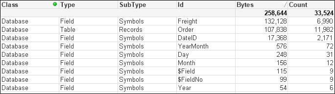
We can see the values for Year, Month, and Day have a very low count. It is worth noting here that Year takes up a lot less space than Month or Day; this is because Year is just an integer and the others are Dual values that have text as well as numbers.
Let's modify the script to have the date fields in a different table in the following manner:
Order:
LOAD AutoNumber(OrderID, 'Order') As OrderID,
     Floor(OrderDate) As DateID,
     AutoNumber(CustomerID, 'Customer') As CustomerID,
     AutoNumber(EmployeeID, 'Employee') As EmployeeID,
     Freight
FROM
[..\Scripts\OrderHeader.qvd]
(qvd);

Calendar:
Load Distinct
     DateID,
     Date(DateID) As Date,
     Year(DateID) As Year,
     Month(DateID) As Month,
     Day(DateID) As Day,
     Date(MonthStart(DateID), 'YYYY-MM') As YearMonth
Resident
   Order;
We can see that there is a difference in the memory profile:
We have all the same symbol table values that we had before with the same memory. We do have a new data table for Calendar, but it is only quite small because there are only a small number of values. We have, however, made a dent in the size of the Order table because we have removed pointers from it. This effect will be increased as the number of rows increases in the Order table, whereas the number of rows in the Calendar table will not increase significantly over time.
Of course, because the data is now in two tables, there will be a potential downside in that joins will need to be made between the tables to answer queries. However, we should always prefer to have a smaller memory footprint. But how can we tell if there was a difference in performance?
As well as information about memory use in each data table and symbol table, we can recall that the Memory Statistics option will also export information about charts—both memory use and calculation time. This means that we can create a chart, especially one with multiple dimensions and expressions, and see how long the chart takes to calculate for different scenarios.
Let's load the Order Header and Order Line data with the Calendar information loaded inline (as in the first part of the last example) in the following manner:
Order:
LOAD AutoNumber(OrderID, 'Order') As OrderID,
     Floor(OrderDate) As DateID,
     Year(OrderDate) As Year,
     Month(OrderDate) As Month,
     Day(OrderDate) As Day,
     Date(MonthStart(OrderDate), 'YYYY-MM') As YearMonth,
     AutoNumber(CustomerID, 'Customer') As CustomerID,
     AutoNumber(EmployeeID, 'Employee') As EmployeeID,
     Freight
FROM
[..\Scripts\OrderHeader.qvd]
(qvd);


OrderLine:
LOAD AutoNumber(OrderID, 'Order') As OrderID,
     LineNo,
     ProductID,
     Quantity,
     SalesPrice,
     SalesCost,
     LineValue,
     LineCost
FROM
[..\Scripts\OrderLine.qvd]
(qvd);
Now we can add a chart to the document with several dimensions and expressions like this:
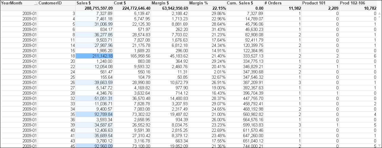
We have used YearMonth and CustomerID as dimensions. This is deliberate because these two fields will be in separate tables once we move the calendar fields into a separate table.
The expressions that we have used are shown in the following table:
|
Expression Label |
Expression |
|---|---|
|
|
|
|
|
|
|
|
|
|
|
|
|
|
|
|
|
|
|
|
|
|
|
|
|
|
|
The cache in QlikView is enormously important. Calculations and selections are cached as you work with a QlikView document. The next time you open a chart with the same selections, the chart will not be recalculated; you will get the cached answer instead. This really speeds up QlikView performance. Even within a chart, you might have multiple expressions using the same calculation (such as dividing two expressions by each other to obtain a ratio)—the results will make use of caching.
This caching is really useful for a working document, but a pain if we want to gather statistics on one or more charts. With the cache on, we need to close a document and the QlikView desktop, reopen the document in a new QlikView instance, and open the chart. To help us test the chart performance, it can therefore be a good idea to turn off the cache.
Note
Note that you need to be very careful with this dialog as you could break things in your QlikView installation. Turning off the cache is not recommended for normal use of the QlikView desktop as it can seriously interfere with the performance of QlikView. Turning off the cache to gather accurate statistics on chart performance is pretty much the only use case that one might ever come across for turning off the cache. There is a reason why it is a hidden setting!
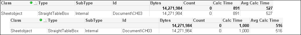
Now that the cache is turned off, we can open our chart and it will always calculate at the maximum time. We can then export the memory information as usual and load it into another copy of QlikView (here, the Class of Sheetobject is selected):

What we could do now is make some selections and save them as bookmarks. By closing the QlikView desktop client and then reopening it, and then opening the document and running through the bookmarks, we can export the memory file and create a calculation for Avg Calc Time. Because there is no cache involved, this should be a valid representation.
Now, we can comment out the inline calendar and create the Calendar table (as we did in a previous exercise):
Order:
LOAD AutoNumber(OrderID, 'Order') As OrderID,
     Floor(OrderDate) As DateID,
//     Year(OrderDate) As Year,
//     Month(OrderDate) As Month,
//     Day(OrderDate) As Day,
//     Date(MonthStart(OrderDate), 'YYYY-MM') As YearMonth,
     AutoNumber(CustomerID, 'Customer') As CustomerID,
     AutoNumber(EmployeeID, 'Employee') As EmployeeID,
     Freight
FROM
[..\Scripts\OrderHeader.qvd]
(qvd);


OrderLine:
//Left Join (Order)
LOAD AutoNumber(OrderID, 'Order') As OrderID,
     LineNo,
     ProductID,
     Quantity,
     SalesPrice,
     SalesCost,
     LineValue,
     LineCost
FROM
[..\Scripts\OrderLine.qvd]
(qvd);

//exit Script;

Calendar:
Load Distinct
    DateID,
     Year(DateID) As Year,
     Month(DateID) As Month,
     Day(DateID) As Day,
     Date(MonthStart(DateID), 'YYYY-MM') As YearMonth
Resident
   Order;
For the dataset size that we are using, we should see no difference in calculation time between the two data structures. As previously established, the second option has a smaller in-memory data size, so that would always be the preferred option.
For many years, it has been a well-established fact among QlikView consultants that a Count() function with a Distinct clause is a very expensive calculation. Over the years, I have heard that Count can be up to 1000 times more expensive than Sum. Actually, since about Version 9 of QlikView, this is no longer true, and the Count function is a lot more efficient.
Note
See Henric Cronström's blog entry at http://community.qlik.com/blogs/qlikviewdesignblog/2013/10/22/a-myth-about-countdistinct for more information.
Count is still a more expensive operation, and the recommended solution is to create a counter field in the table that you wish to count, which has a value of 1. You can then sum this counter field to get the count of rows. This field can also be useful in advanced expressions like
Set Analysis.
Using the same dataset as in the previous example, if we create a chart using similar dimensions (YearMonth and CustomerID) and the same expression for Order # as done previously:
Count(Distinct OrderID)
This gives us a chart like the following:
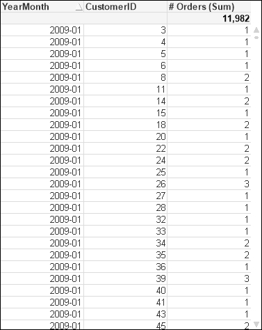
After running through the same bookmarks that we created earlier, we get a set of results like the following:

So, now we modify the Order table load as follows:
Order:
LOAD AutoNumber(OrderID, 'Order') As OrderID,
     1 As OrderCounter,
     Floor(OrderDate) As DateID,
     AutoNumber(CustomerID, 'Customer') As CustomerID,
     AutoNumber(EmployeeID, 'Employee') As EmployeeID,
     Freight
FROM
[..\Scripts\OrderHeader.qvd]
(qvd);
Once we reload, we can modify the expression for Order # to the following:
Sum(OrderCounter)
We close down the document, reopen it, and run through the bookmarks again. This is an example result:

And yes, we do see that there is an improvement in calculation time—it appears to be a factor of about twice as fast.
The amount of additional memory needed for this field is actually minimal. In the way we have loaded it previously, the OrderCounter field will add only a small amount in the symbol table and will only increase the size of the data table by a very small amount—it may, in fact, appear not to increase it at all! The only increase is in the core system tables, and this is minor.
Note
Recalling that data tables are bit-stuffed but stored as bytes, adding a one-bit value like this to the data table may not actually increase the number of bytes needed to store the value. At worst, only one additional byte will be needed.
In fact, we can reduce this minor change even further by making the following change:
     ...
     Floor(1) As OrderCounter,
     ...
This forces the single value to be treated as a sequential integer (a sequence of one) and the value therefore isn't stored in the symbol table.
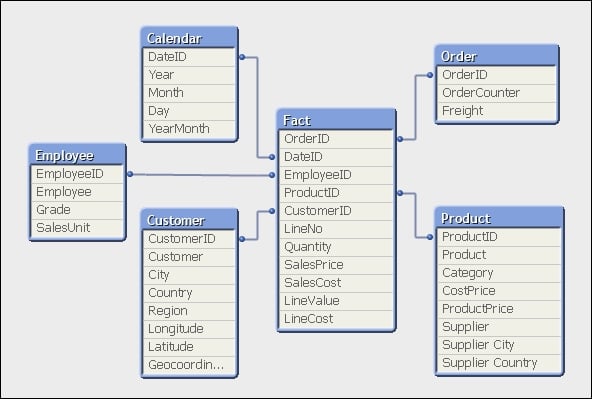
If we load all of our tables, the data structure may look something like the following:
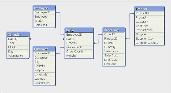
In this format, we have two fact tables—Order and OrderLine. For the small dataset that we have, we won't see any issues here. As the dataset gets larger, it is suggested that it is better to have fewer tables and fewer joins between tables. In this case, between Product and Employee, there are three joins. The best practice is to have only one fact table containing all our key fields and associated facts (measures).
In this model, most of the facts are in the OrderLine table, but there are two facts in the Order table—OrderCounter and Freight. We need to think about what we do with them. There are two options:
Move the
EmployeeID,DateID, andCustomerIDfields from theOrdertable into theOrderLinetable. Create a script based on an agreed business rule (for example, ratio of lineQuantity) to apportion theFreightvalue across all of the line values. TheOrderCounterfield is more difficult to deal with, but we could take the option of usingCount(Distinct OrderID)(knowing that it is less efficient) in the front end and disposing of theOrderCounterfield.This method is more in line with traditional data warehousing methods.
Move the
EmployeeID,DateID, andCustomerIDfields from theOrdertable into theOrderLinetable. Leave theOrdertable as is, as anOrderdimension table.This is more of a QlikView way of doing things. It works very well too.
Although we might be great fans of dimensional modeling methods (see Chapter 2, QlikView Data Modeling), we should also be a big fan of pragmatism and using what works.
Let's see what happens if we go for option 2. The following is the addition to the script to move the key fields:
// Move DateID, CustomerID and EmployeeID to OrderLine
Join (OrderLine)
Load
   OrderID,
   DateID,
   CustomerID,
   EmployeeID
Resident
   Order;

Drop Fields DateID, CustomerID, EmployeeID From Order;

// Rename the OrderLine table
RENAME Table OrderLine to Fact;
So, how has that worked? The table structure now looks like the following:
Our expectation, as we have widened the biggest data table (OrderLine) and only narrowed a smaller table (Order), is that the total memory for the document will be increased. This is confirmed by taking memory snapshots before and after the change:
But have we improved the overall performance of the document?
To test this, we can create a new version of our original chart, except now using Customer instead of CustomerID and adding Product. This gives us fields (YearMonth, Customer, and Product) from across the dimension tables. If we use this new straight table to test the before and after state, the following is how the results might look:
Interestingly, the average calculation has reduced slightly. This is not unexpected as we have reduced the number of joins needed across data tables.
QlikView has a great feature in that it can sometimes default to storing numbers as Dual values—the number along with text representing the default presentation of that number. This text is derived either by applying the default formats during load, or by the developer applying formats using functions such as Num(), Date(), Money(), or TimeStamp(). If you do apply the format functions with a format string (as the second parameter to Num, Date, and so on), the number will be stored as a Dual. If you use Num without a format string, the number will usually be stored without the text.
Thinking about it, numbers that represent facts (measures) in our fact tables will rarely need to be displayed with their default formats. They are almost always only ever going to be displayed in an aggregation in a chart and that aggregated value will have its own format. The text part is therefore superfluous and can be removed if it is there.
Let's modify our script in the following manner:
Order:
LOAD AutoNumber(OrderID, 'Order') As OrderID,
     Floor(1) As OrderCounter,
     Floor(OrderDate) As DateID,
     AutoNumber(CustomerID, 'Customer') As CustomerID,
     AutoNumber(EmployeeID, 'Employee') As EmployeeID,
     Num(Freight) As Freight
FROM
[..\Scripts\OrderHeader.qvd]
(qvd);


OrderLine:
LOAD AutoNumber(OrderID, 'Order') As OrderID,
     LineNo,
     ProductID,
     Num(Quantity) As Quantity,
     Num(SalesPrice) As SalesPrice,
     Num(SalesCost) As SalesCost,
     Num(LineValue) As LineValue,
     Num(LineCost) As LineCost
FROM
[..\Scripts\OrderLine.qvd]
(qvd);
The change in memory looks like the following:
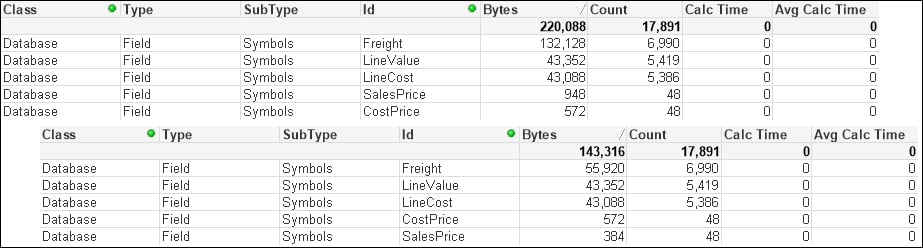
We can see that there is a significant difference in the Freight field. The smaller SalesPrice field has also been reduced. However, the other numeric fields are not changed.
Some numbers have additional format strings and take up a lot of space, some don't. Looking at the numbers, we can see that the Freight value with the format string is taking up an average of over 18 bytes per value. When Num is applied, only 8 bytes are taken per value. Let's add an additional expression to the chart:
|
Expression label |
Expression |
|---|---|
|
|
|
Now we have a quick indicator to see whether numeric values are storing unneeded text.
Once we have optimized our data model, we can turn our focus onto chart performance. There are a few different things that we can do to make sure that our expressions are optimal, and we can use the memory file extract to test them.
Some of the expressions will actually involve revisiting the data model. If we do, we will need to weigh up the cost of that performance with changes to memory, and so on.
It will be useful to begin with an explanation of how the QlikView calculation engine works.
QlikView is very clever in how it does its calculations. As well as the data storage, as discussed earlier in this chapter, it also stores the binary state of every field and of every data table dependent on user selection—essentially, depending on the green/white/grey state of each field, it is either included or excluded. This area of storage is called the state space and is updated by the QlikView logical inference engine every time a selection is made. There is one bit in the state space for every value in the symbol table or row in the data table—as such, the state space is much smaller than the data itself and hence much faster to query.
There are three steps to a chart being calculated:
The user makes a selection, causing the logical inference engine to reset and recalculate the state space. This should be a multithreaded operation.
On one thread per object, the state space is queried to gather together all of the combinations of dimensions and values necessary to perform the calculation. The state space is being queried, so this is a relatively fast operation, but could be a potential bottleneck if there are many visible objects on the screen.
On multiple threads per object, the expression is calculated. This is where we see the cores in the task manager all go to 100 percent at the same time. Having 100 percent CPU is expected and desired because QlikView will "burst" calculations across all available processor cores, which makes this a very fast process, relative to the size and complexity of the calculation. We call it a burst because, except for the most complex of calculations, the 100 percent CPU should only be for a short time.
Of course, the very intelligent cache comes into play as well and everything that is calculated is stored for potential subsequent use. If the same set of selections are met (such as hitting the Back button), then the calculation is retrieved from the cache and will be almost instantaneous.
Now that we know more about how QlikView performs its calculations, we can look at a few ways that we can optimize things.
We cannot anticipate every possible selection or query that a user might make, but there are often some quite well-known conditions that will generally be true most of the time and may be commonly used in calculations. In this example, we will look at Year-to-Date and Last Year-to-Date—commonly used on dashboards.
The following is an example of a calculation that might be used in a gauge:
Sum(If(YearToDate(Date), LineValue, 0))
/Sum(If(YearToDate(Date,-1), LineValue, 0))
-1
This uses the YearToDate() function to check whether the date is in the current year to date or in the year to date period for last year (using the -1 for the offset parameter). This expression is a sum of an if statement, which is generally not recommended. Also, these are quite binary—a date is either in the year to date or not—so are ideal candidates for the creation of flags. We can do this in the Calendar table in the following script:
Calendar:
Load Distinct
     DateID,
     -YearToDate(DateID) As YTD_Flag,
     -YearToDate(DateID,-1) As LYTD_Flag,
     Date(DateID) As Date,
     Year(DateID) As Year,
     Month(DateID) As Month,
     Day(DateID) As Day,
     Date(MonthStart(DateID), 'YYYY-MM') As YearMonth
Resident
   Order;
Note
Note the - sign before the function. This is because YearToDate is a Boolean function that returns either true or false, which in QlikView is represented by -1 and 0. If the value is in the year to date, then the function will return -1, so I add the - to change that to 1. A - sign before 0 will make no difference.
In a particular test dataset, we might see an increase from 8,684 bytes to 13,026—not an unexpected increase and not significant because the Calendar table is relatively small. We are creating these flags to improve performance in the frontend and need to accept a small change in the data size.
The significant change comes when we change the expression in the chart to the following:
Sum(LineValue*YTD_Flag)/Sum(LineValue*LYTD_Flag)-1
In a sample dataset, we might see that the calculation reduces from, say, 46 to, say, 16—a 65 percent reduction. This calculation could also be written using Set Analysis as follows:
Sum({<YTD_Flag={1}>} LineValue)/Sum({<LYTD_Flag={1}>} LineValue)-1However, this might only get a calc time of 31—only a 32.6 percent reduction. Very interesting!
If we think about it, the simple calculation of LineValue*YTD_Flag is going to do a multithreaded calculation using values that are derived from the small and fast in-memory state space. Both If and Set Analysis are going to add additional load to the calculation of the set of values that are going to be used in the calculation.
In this case, the flag field is in a dimension table, Calendar, and the value field is in the fact table. It is, of course, possible to generate the flag field in the fact table instead. In this case, the calculation is likely to run even faster, especially on very large datasets. This is because there is no join of data tables required. However, the thing to bear in mind is that the additional pointer indexes in the Calendar table will require relatively little space whereas the additional width of the fact table, because of the large numbers of rows, will be something to consider. However, saying that, the pointers to the flag values are very small, so you do need a really long fact table for it to make a big difference. In some cases, the additional bit necessary to store the pointer in the bit-stuffed table will not make any difference at all, and in other cases, it may add just one byte.
Set Analysis can be very powerful, but it is worth considering that it often has to go, depending on the formula, outside the current state space, and that will cause additional calculation to take place that may be achieved in a simpler manner by creating a flag field in the script and using it in this way. Even if you have to use Set Analysis, the best performing comparisons are going to be using numeric comparisons, so creating a numeric flag instead of a text value will improve the set calculation performance. For example, consider the following expression:
Sum({<YTD_Flag={1}>} LineValue)This will execute much faster than the following expression:
Sum({<YTD_Flag={'Yes'}>} LineValue)So, when should we use Set Analysis instead of multiplying by flags? Barry Harmsen has done some testing that indicates that if the dimension table is much larger relative to the fact table, then using Set Analysis is faster than the flag fields. The reasoning is that the multiply method will process all records (even those containing 0), so in larger tables, it has more to process. The Set Analysis method will first reduce the scope, and apply the calculation to that subset.
Of course, if we have to introduce more advanced logic, that might include AND/OR/NOT operations, then Set Analysis is the way to go—but try to use numeric flags.
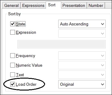
Any time that you need to sort a chart or listbox, that sort needs to be calculated. Of course, a numeric sort will always be the fastest. An alphabetic sort is a lot slower, just by its nature. One of the very slowest sorts is where we want to sort by expression.
For example, let's imagine that we wish to sort our Country list by a fixed order, defined by the business. We could use a sort expression like this:
Match(Country,'USA','Canada','Germany','United Kingdom','China','India','Russia','France','Ireland')
The problem is that this is a text comparison that will be continually evaluated. What we can do instead is to load a temporary sort table in the script. We load this towards the beginning of the script because it needs to be the initial load of the symbol table; something like the following:
Country_Sort:
Load * Inline [
Country
USA
Canada
Germany
United Kingdom
China
India
Russia
France
Ireland
];
Then, as we won't need this table in our data, we should remember to drop it at the end of the script—after the main data has been loaded:
Drop Table Country_Sort;
Now, when we use this field anywhere, we can turn off all of the sort options and use the last one—Load Order. This doesn't need to be evaluated so will always calculate quickly:
Traditionally, QlikView has been a totally in-memory tool. If you want to analyze any information, you need to get all of the data into memory. This has caused problems for many enterprise organizations because of the sheer size of data that they wanted to analyze. You can get quite a lot of data into QlikView—billions of rows are not uncommon on very large servers, but there is a limit. Especially in the last few years where businesses have started to take note of the buzz around Big Data, many believed that QlikView could not play in this area.
Direct Discovery was introduced with QlikView Version 11.20. In Version 11.20 SR5, it was updated with a new, more sensible syntax. This syntax is also available in Qlik Sense. What Direct Discovery does is allow a QlikView model to connect directly to a data source without having to load all of the data into memory. Instead, we load only dimension values and, when necessary, QlikView generates a query to retrieve the required results from the database.
Of course, this does have the potential to reduce some of the things that make QlikView very popular—the sub-second response to selections, for example. Every time that a user makes a selection, QlikView generates a query to pass through to the database connection. The faster the data connection, the faster the response, so a performative data warehouse is a boon for Direct Discovery. But speed is not always everything—with Direct Discovery, we can connect to any valid connection that we might normally connect to with the QlikView script; this includes ODBC connectors to Big Data sources such as Cloudera or Google.
Note
Here we will get an introduction to using Direct Discovery, but we should read the more detailed technical details published by the Qlik Community, for example, the SR5 technical addendum at http://community.qlik.com/docs/DOC-3710.
There are a few restrictions of Direct Discovery that will probably be addressed with subsequent service releases:
Only one direct table is supported: This restriction has been lifted in QlikView 11.20 SR7 and Qlik Sense 1.0. Prior to those versions, you could only have one direct query in your data model. All other tables in the data model must be in-memory.
Set Analysis and complex expressions not supported: Because the query is generated on the fly, it just can't work with the likes of a
Set Analysisquery. Essentially, only calculations that can be performed on the source database—Sum,Count,Avg,Min,Max—will work via Direct Discovery.Only SQL compliant data sources: Direct Discovery will only work against connections that support SQL, such as ODBC, OLEDB, and custom connectors such as SAP and JDBC. Note that there are some system variables that may need to be set for some connectors, such as SAP or Google Big Query.
Direct fields are not supported in global search: Global search can only operate against in-memory data.
Security restrictions: Prior to QlikView 11.20 SR7 and Qlik Sense 1.0, Section Access reduction can work on the in-memory data, but will not necessarily work against the
Directtable. Similarly,LoopandReduceinPublisherwon't work correctly.Synthetic keys not supported: You can only have native key associations.
AutoNumberwill obviously not be supported on the direct table.Calculated dimensions not supported: You can only create calculated dimensions against in-memory data.
Naming the Direct table: You can't create a table alias. The table will always be called
DirectTable.
It is also worth knowing that QlikView will use its cache to store the results of queries. So if you hit the Back button, the query won't be rerun against the source database. However, this may have consequences when the underlying data is updated more rapidly. There is a variable—DirectCacheSeconds—that can be set to limit the time that data is cached. This defaults to 3600 seconds.
The most important statement is the opening one:
DIRECT QUERY
This tells QlikView to expect some further query components. It is similar to the SQL statement that tells QlikView to execute the subsequent query and get the results into the memory. The DIRECT QUERY is followed by:
DIMENSION Dim_1, Dim_2, ..., Dim_n
We must have at least one dimension field. These fields will have their values loaded into a symbol table and state space. This means that they can be used as normal in listboxes, tables, charts, and so on. Typically, the DIMENSION list will be followed by:
MEASURE Val_1, Val_2, ..., Val_n
These fields are not loaded into the data model. They can be used, however, in expressions. You can also have additional fields that are not going to be used in expressions or dimensions:
DETAIL Note_1, Note_2, ..., Note_n
These DETAIL fields can only be used in table boxes to give additional context to other values. This is useful for text note fields.
Finally, there may be fields that you want to include in the generated SQL query but are not interested in using in the QlikView model:
DETACH other_1, other_2, ..., other_n
Finally, you can also add a limitation to your query using a standard WHERE clause:
WHERE x=y
The statement will, of course, be terminated by a semicolon.
We can also pass valid SQL syntax statements to calculate dimensions:
NATIVE('Valid SQL ''syntax'' in quotes') As Field_xIf your SQL syntax also has single quotes, then you will need to double-up on the single quotes to have it interpreted correctly.
The following is an example of a Direct Query to a SQL server database:
DIRECT QUERY
dimension
   OrderID,
   FLOOR(OrderDate) As DateID,
    CustomerID,
    EmployeeID,
    ProductID
measure
    Quantity,
    SalesPrice,
    LineValue,
    LineCost
detail
    Freight,
    LineNo
FROM QWT.dbo."Order_Fact";
This results in a table view like the following:
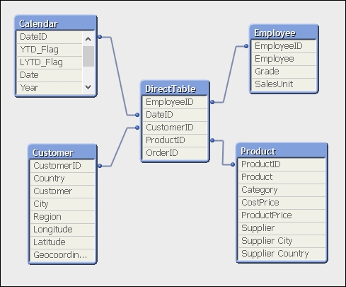
You will note that the list of fields in the table view only contains the dimension values. The measure values are not shown.
You can now go ahead and build charts mostly as normal (without, unfortunately, Set Analysis!), but note that you will see a lot more of the hourglass:
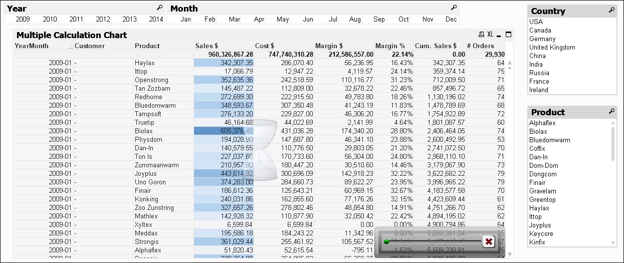
The X in the bottom corner of the chart can be used to cancel the execution of the direct query.
JMeter is a tool from Apache that can be used to automate web-based interactions for the purpose of testing scalability. Basically, we can use this tool to automatically connect to a QlikView application, make different selections, look at different charts, drill up and down, and repeat to test how well the application performs.
JMeter first started being used for testing QlikView about 3 years ago. At the time, while it looked like a great tool, the amount of work necessary to set it up was very off-putting.
Since then, however, the guys in the Qlik scalability center have created a set of tools that automate the configuration of JMeter, and this makes things a lot easier for us. In fact, almost anyone can set up a test—it is that easy!
The tools needed to test scalability are made available via the Qlik community. You will need to connect to the Scalability group (http://community.qlik.com/groups/qlikview-scalability).
Search in this group for "tools" and you should find the latest version. There are some documents that you will need to read through, specifically:
Prerequisites.pdfQVScalabilityTools.pdf
JMeter can be obtained from the Apache website:
However, the prerequisites documentation recommends a slightly older version of JMeter:
http://archive.apache.org/dist/jakarta/jmeter/binaries/jakarta-jmeter-2.4.zip
JMeter is a Java application, so it is also a good idea to make sure that you have the latest version of the Java runtime installed—64-bit for a 64-bit system:
http://java.com/en/download/manual.jsp
It is recommended not to unzip JMeter directly to C:\ or Program Files or other folders that may have security that reduces your access. Extract them to a folder that you have full access to. Do note the instructions in the Prerequisites.pdf file on setting heap memory sizing. To confirm that all is in order, you can try running the jmeter.bat file to open JMeter—if it works, then it means that your Java and other dependencies should be installed correctly.
Microsoft .Net 4.0 should also be installed on the machine. This can be downloaded from Microsoft. However, it should already be installed if you have QlikView Server components on the machine.
Depending on your system, you may find that the ZIP file that you download has its status set to Blocked. In this case, you need to right-click on the file, open the properties, and click on the Unblock button:
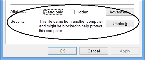
If you don't, you may find that the file appears to unzip successfully, but the executables will not run. You might see an error like this in the Windows Application Event Log:
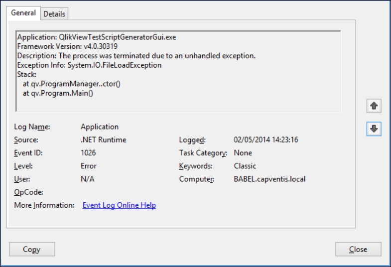
After you have made sure that the ZIP file is unblocked, you can extract the scalability tools to a folder on your system. Follow the instructions in the Prerequisites.pdf file to change the configuration.
Running a session is actually quite straightforward, and a lot easier than having to craft the script by hand.
There are a couple of steps that we need to do before we can generate a test script:
We need to open the target application in QlikView desktop and extract the layout information:

This exports all of the information about the document, including all of the objects, into XML files that can be imported into the script generator. This is how the script generator finds out about sheets and objects that it can use.
Copy the
AjaxZfcURL for the application. We need to give this information to the script builder so that it knows how to connect to the application:
Clear the existing log files from the QVS. These files will be in the
ProgramData\QlikTech\QlikViewServerfolder. Stop the QlikView Server Service and then archive or delete thePerformance*.log,Audit*.log,Events*.log, andSessions*.logfiles. When you restart the service, new ones will start to be created:
Start the Performance Monitor using the template that you configured earlier. Double-check that it starts to create content in the folder (for example,
C:\PerfLogs\Admin\New Data Collector Set\QlikView Performance Monitor).
Once those steps have been completed, we can go ahead and create a script:
Execute the script generator by running
QlikViewTestScriptGeneratorGui.exefrom theScriptGeneratorfolder.
There are some properties that we need to set on this page:
Property
Value
QlikView version
11.
Document URL
Paste the URL that you recorded earlier.
Security settings
Choose the right authentication mechanism for your QlikView server (more details discussed later).
Concurrent users
How many users you want to run concurrently.
Iterations per user
How many times each user will run through the scenario. If you set this to Infinite, you need to specify a Duration below.
Ramp up
What time should there be before all users are logged in. 1 means that all users start together.
Duration
How long the test should be run for. If you set this to Infinite then you must set a number of Iterations per user above it.
Note
If you use NTLM, then you cannot use more than one concurrent user. This is because the NTLM option will execute under the profile of the user running the application and each concurrent user will therefore attempt to log in with the same credentials. QVS does not allow this so each concurrent user will actually end up killing each other's sessions.
If you want to simulate more than one user, then you can turn on Header authentication in the QVWS configuration and make use of the
userpw.txtfile to add a list of users. The QVS will need to be in DMS mode to support this. Also bear in mind that you will need to have an appropriate number of licenses available to support the number of users that you want to test with.Save the document in the
ScriptGenerator\SourceXMLsfolder. Note that you should not use spaces or non-alphanumeric characters in the XML filename. It is a good idea to make the filename descriptive as you might use it again and again.Click the Scenario tab. Click the Browse button and navigate to the folder where you save the document layout information earlier. Save the template (it's always a good idea to save continually as you go along). Change the Timer Delay Min to 30 and the Max to 120:

This setting specifies the range of delay between different actions. We should always allow an appropriate minimum to make sure that the application can update correctly after an action. The random variation between the minimum and maximum settings gives a simulation of user thinking time.
By default, there are three default actions—open AccessPoint, open the document, and then a timer delay. Click on the green + button on the left-hand side of the bottom timer delay action to add a new action below it. Two new actions will be added—an unspecified Choose Action one and a timer delay containing the settings that we specified above. The Auto add timers checkbox means that a timer delay will be automatically added every time we add a new action.
Build up a scenario by adding appropriate actions:

Remember to keep saving as you go along.
Click on the Execution tab. Click on Yes in answer to the Add to execution prompt. Expand the Settings option and click on Browse to select the JMeter path:

When you click on OK, you will be prompted on whether to save this setting permanently or not. You can click on OK in response to this message:
Right-click on the script name and select Open in JMeter:

Click on OK on OutputPopupForm. When JMeter opens, note the entries that have been created in the test plan by the script generator.

Close JMeter. Back in the script generator, right-click on the script again and select Run from the menu. The Summary tab appears, indicating that the script is executing:

Once you have executed a test, you will want to analyze the results. The scalability tools come with a couple of QVW files to help you out here. There are a couple of steps that you need to go through to gather all the files together first:
In the
QVScriptGenTool_0_7 64Bit\Analyzerfolder, there is a ZIP file calledFolderTemplate.zip. Extract theFolderTemplatefolder out of the ZIP file and rename it to match the name of your analysis task—for example,SalesAnalysis. Within this folder, there are four subfolders that you need to populate with data:Subfolder
Data source
EventLogsThese are the QVS event logs—
Events_servername_*.logJMeterLogsThese are the JMeter execution logs that should be in
QVScriptGenTool_0_7 64Bit\Analyzer\JMeterExecutionsServerLogsThese are the CSV files created—
SERVERNAME_Processes*.csvSessionLogsThese are the QVS session logs—
Sessions_servername_*.logOpen the
QVD Generator.qvwfile using QlikView Desktop. Set the correct name for the subfolder that you have just created:
Reload the document.
Once the document has reloaded, manually edit the name of the server using the input fields in each row of the table:

Once you have entered the data, click on the Create Meta-CSV button. You can then close the QVD Generator.
Open the
SC_Results – DemoTest.qvwfile and save it as a new file with an appropriate name—for example,SC_Results – SalesAnalysis.qvw. Change the Folder Name variable as before and reload.
Now you can start to analyze your server's performance during the tests:
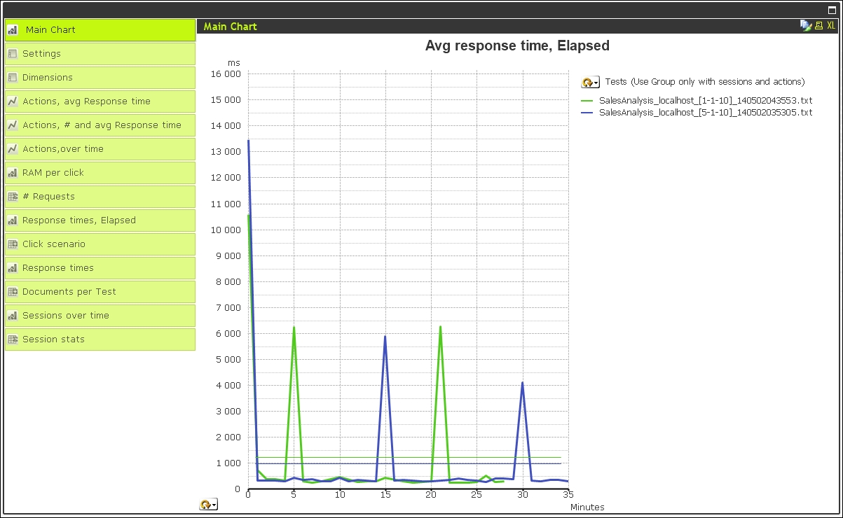
Because you can run multiple iterations of the test, with different parameters, you can use the tool to run comparisons to see changes. These can also be scheduled from the command line to run on a regular basis.
Note
One thing that these JMeter scripts can be used for is a process called "warming the cache". If you have a very large QlikView document, it can take a long time to load into memory and create the user cache. For the first users to connect to the document in the morning, they may have a very poor experience while waiting for the document to open—they may even time out. Subsequent users will get the benefit of these user actions. However, if you have a scheduled task to execute a JMeter task, you can take the pain away from those first users because the cache will already be established for them when they get to work.
There has been a lot of information in this chapter, and I hope that you have been able to follow it well.
We started by reviewing some basic performance improvement techniques that you should already have been aware of, but you might not think about. Knowing these techniques is important and is the beginning of your path to mastering how to create performative QlikView applications.
We then looked at methods of generating test data that can be used to help you hone your skills.
Understanding how QlikView stores its data is a real requisite for any developer who wants to achieve mastery of this subject. Learning how to export memory statistics is a great step forward to learn how to achieve great things with performance and scalability.
We looked at different strategies for reducing the memory profile of a QlikView application and improving the performance of charts.
By this stage, you should have a great start in understanding how to create really performative applications.
When it gets to the stage where there is just too much data for QlikView to manage in-memory, we have seen that we can use a hybrid approach where some of the data is in-memory and some of the data is still in a database, and we can query that data on the fly using Direct Discovery.
Finally, we looked at how we can use JMeter to test our applications with some real-world scenarios using multiple users and repetitions to really hammer an application and confirm that it will work on the hardware that is in place.
Having worked through this chapter, you should have a great understanding of how to create scalable applications that perform really well for your users. You are starting to become a QlikView master!
In the next chapter, we will learn about best practices in modeling data and how that applies to QlikView.