


In this chapter, we consider some advanced time series methods and their implementation using R. Time series analysis, as a discipline, is broad enough to fill hundreds of books (the most important references, both in theory and R programming, will be listed at the end of this chapter's reading list); hence, the scope of this chapter is necessarily highly selective, and we focus on topics that are inevitably important in empirical finance and quantitative trading. It should be emphasized at the beginning, however, that this chapter only sets the stage for further studies in time series analysis.
Our previous book Introduction to R for Quantitative Finance, Packt Publishing, discusses some fundamental topics of time series analysis such as linear, univariate time series modeling, Autoregressive integrated moving average (ARIMA), and volatility modeling Generalized Autoregressive Conditional Heteroskedasticity (GARCH). If you have never worked with R for time series analysis, you might want to consider going through Chapter 1, Time Series Analysis of that book as well.
The current edition goes further in all of these topics and you will become familiar with some important concepts such as cointegration, vector autoregressive models, impulse-response functions, volatility modeling with asymmetric GARCH models including exponential GARCH and Threshold GARCH models, and news impact curves. We first introduce the relevant theories, then provide some practical insights to multivariate time series modeling, and describe several useful R packages and functionalities. In addition, using simple and illustrative examples, we give a step-by-step introduction to the usage of R programming language for empirical analysis.
The basic issues regarding the movements of financial asset prices, technical analysis, and quantitative trading are usually formulated in a univariate context. Can we predict whether the price of a security will move up or down? Is this particular security in an upward or a downward trend? Should we buy or sell it? These are all important considerations; however, investors usually face a more complex situation and rarely see the market as just a pool of independent instruments and decision problems.
By looking at the instruments individually, they might seem non-autocorrelated and unpredictable in mean, as indicated by the Efficient Market Hypothesis, however, correlation among them is certainly present. This might be exploited by trading activity, either for speculation or for hedging purposes. These considerations justify the use of multivariate time series techniques in quantitative finance. In this chapter, we will discuss two prominent econometric concepts with numerous applications in finance. They are cointegration and vector autoregression models.
From now on, we will consider a vector of time series  , which consists of the elements
 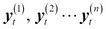 each of them individually representing a time series, for instance, the price evolution of different financial products. Let's begin with the formal definition of cointegrating data series.
The  vector of time series is said to be cointegrated if each of the series are individually integrated in the order
  (in particular, in most of the applications the series are integrated of order 1, which means nonstationary unit-root processes, or random walks), while there exists a linear combination of the series
  , which is integrated in the order
  (typically, it is of order 0, which is a stationary process).
Intuitively, this definition implies the existence of some underlying forces in the economy that are keeping together the n time series in the long run, even if they all seem to be individually random walks. A simple example for cointegrating time series is the following pair of vectors, taken from Hamilton (1994), which we will use to study cointegration, and at the same time, familiarize ourselves with some basic simulation techniques in R:
The unit root in will be shown formally by standard statistical tests. Unit root tests in R can be performed using either the tseries package or the urca package; here, we use the second one. The following R code simulates the two series of length 1000:
#generate the two time series of length 1000

set.seed(20140623)         #fix the random seed
N <- 1000                  #define length of simulation
x <- cumsum(rnorm(N))      #simulate a normal random walk
gamma <- 0.7               #set an initial parameter value
y <- gamma * x + rnorm(N)  #simulate the cointegrating series
plot(x, type='l')          #plot the two series
lines(y,col="red")
Tip
Downloading the example code
You can download the example code files from your account at http://www.packtpub.com for all the Packt Publishing books you have purchased. If you purchased this book elsewhere, you can visit http://www.packtpub.com/support and register to have the files e-mailed directly to you.
The output of the preceding code is as follows:
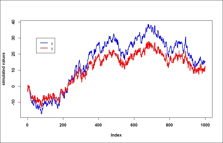
By visual inspection, both series seem to be individually random walks. Stationarity can be tested by the Augmented Dickey Fuller test, using the urca package; however, many other tests are also available in R. The null hypothesis states that there is a unit root in the process (outputs omitted); we reject the null if the test statistic is smaller than the critical value:
#statistical tests
install.packages('urca');library('urca')
#ADF test for the simulated individual time series
summary(ur.df(x,type="none"))
summary(ur.df(y,type="none"))
For both of the simulated series, the test statistic is larger than the critical value at the usual significance levels (1 percent, 5 percent, and 10 percent); therefore, we cannot reject the null hypothesis, and we conclude that both the series are individually unit root processes.
Now, take the following linear combination of the two series and plot the resulted series:
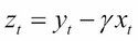
z = y - gamma*x	#take a linear combination of the series
plot(z,type='l')
The output for the preceding code is as follows:
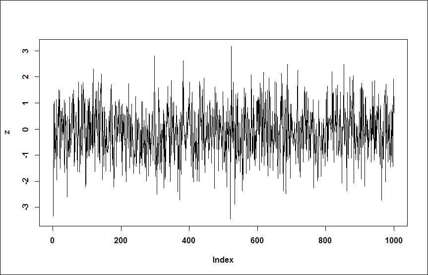
 clearly seems to be a white noise process; the rejection of the unit root is confirmed by the results of ADF tests:
summary(ur.df(z,type="none"))
In a real-world application, obviously we don't know the value of  ; this has to be estimated based on the raw data, by running a linear regression of one series on the other. This is known as the Engle-Granger method of testing cointegration. The following two steps are known as the Engle-Granger method of testing cointegration:


Tip
We should note here that in the case of the n series, the number of possible independent cointegrating vectors is  ; therefore, for
  , the cointegrating relationship might not be unique. We will briefly discuss
  later in the chapter.
Simple linear regressions can be fitted by using the lm function. The residuals can be obtained from the resulting object as shown in the following example. The ADF test is run in the usual way and confirms the rejection of the null hypothesis at all significant levels. Some caveats, however, will be discussed later in the chapter:
#Estimate the cointegrating relationship
coin <- lm(y ~ x -1)           #regression without intercept
coin$resid                     #obtain the residuals
summary(ur.df(coin$resid))     #ADF test of residuals
Now, consider how we could turn this theory into a successful trading strategy. At this point, we should invoke the concept of statistical arbitrage or pair trading, which, in its simplest and early form, exploits exactly this cointegrating relationship. These approaches primarily aim to set up a trading strategy based on the spread between two time series; if the series are cointegrated, we expect their stationary linear combination to revert to 0. We can make profit simply by selling the relatively expensive one and buying the cheaper one, and just sit and wait for the reversion.
Tip
The term statistical arbitrage, in general, is used for many sophisticated statistical and econometrical techniques, and this aims to exploit relative mispricing of assets in statistical terms, that is, not in comparison to a theoretical equilibrium model.
What is the economic intuition behind this idea? The linear combination of time series that forms the cointegrating relationship is determined by underlying economic forces, which are not explicitly identified in our statistical model, and are sometimes referred to as long-term relationships between the variables in question. For example, similar companies in the same industry are expected to grow similarly, the spot and forward price of a financial product are bound together by the no-arbitrage principle, FX rates of countries that are somehow interlinked are expected to move together, or short-term and long-term interest rates tend to be close to each other. Deviances from this statistically or theoretically expected comovements open the door to various quantitative trading strategies where traders speculate on future corrections.
The concept of cointegration is further discussed in a later chapter, but for that, we need to introduce vector autoregressive models.
Vector autoregressive models (VAR) can be considered as obvious multivariate extensions of the univariate autoregressive (AR) models. Their popularity in applied econometrics goes back to the seminal paper of Sims (1980). VAR models are the most important multivariate time series models with numerous applications in econometrics and finance. The R package vars provide an excellent framework for R users. For a detailed review of this package, we refer to Pfaff (2013). For econometric theory, consult Hamilton (1994), Lütkepohl (2007), Tsay (2010), or Martin et al. (2013). In this book, we only provide a concise, intuitive summary of the topic.
In a VAR model, our point of departure is a vector of time series of length  . The VAR model specifies the evolution of each variable as a linear function of the lagged values of all other variables; that is, a VAR model of the order p is the following:
Here,  are
are  the coefficient matrices for all
  , and
, and  is a vector white noise process with a positive definite covariance matrix. The terminology of vector white noise assumes lack of autocorrelation, but allows contemporaneous correlation between the components; that is, has a non-diagonal covariance matrix.
The matrix notation makes clear one particular feature of VAR models: all variables depend only on past values of themselves and other variables, meaning that contemporaneous dependencies are not explicitly modeled. This feature allows us to estimate the model by ordinary least squares, applied equation-by-equation. Such models are called reduced form VAR models, as opposed to structural form models, discussed in the next section.
Obviously, assuming that there are no contemporaneous effects would be an oversimplification, and the resulting impulse-response relationships, that is, changes in the processes followed by a shock hitting a particular variable, would be misleading and not particularly useful. This motivates the introduction of structured VAR (SVAR) models, which explicitly models the contemporaneous effects among variables:
Here,  and
and  ; thus, the structural form can be obtained from the reduced form by multiplying it with an appropriate parameter matrix
  , which reflects the contemporaneous, structural relations among the variables.
Tip
In the notation, as usual, we follow the technical documentation of the vars package, which is very similar to that of Lütkepohl (2007).
In the reduced form model, contemporaneous dependencies are not modeled; therefore, such dependencies appear in the correlation structure of the error term, that is, the covariance matrix of  , denoted by
  . In the SVAR model, contemporaneous dependencies are explicitly modelled (by the A matrix on the left-hand side), and the disturbance terms are defined to be uncorrelated, so the
  covariance matrix is diagonal. Here, the disturbances are usually referred to as structural shocks.
What makes the SVAR modeling interesting and difficult at the same time is the so-called identification problem; the SVAR model is not identified, that is, parameters in matrix A cannot be estimated without additional restrictions.
Tip
How should we understand that a model is not identified? This basically means that there exist different (infinitely many) parameter matrices, leading to the same sample distribution; therefore, it is not possible to identify a unique value of parameters based on the sample.
Given a reduced form model, it is always possible to derive an appropriate parameter matrix, which makes the residuals orthogonal; the covariance matrix  is positive semidefinitive, which allows us to apply the LDL decomposition (or alternatively, the Cholesky decomposition). This states that there always exists an
  lower triangle matrix and a
  diagonal matrix such that
  . By choosing
  , the covariance matrix of the structural model becomes
  , which gives
  . Now, we conclude that
  is a diagonal, as we intended. Note that by this approach, we essentially imposed an arbitrary recursive structure on our equations. This is the method followed by the
 irf() function by default.
There are multiple ways in the literature to identify SVAR model parameters, which include short-run or long-run parameter restrictions, or sign restrictions on impulse responses (see, for example, Fry-Pagan (2011)). Many of them have no native support in R yet. Here, we only introduce a standard set of techniques to impose short-run parameter restrictions, which are respectively called A-model, B-model, and AB-model, each of which are supported natively by package vars:
-
In the case of an A-model,
 , and restrictions on matrix A are imposed such that
  is a diagonal covariance matrix. To make the model "just identified", we need
  additional restrictions. This is reminiscent of imposing a triangle matrix (but that particular structure is not required).
-
Alternatively, it is possible to identify the structural innovations based on the restricted model residuals by imposing a structure on the matrix B (B-model), that is, directly on the correlation structure, in this case,
 and
and  .
.
-
The AB-model places restrictions on both A and B, and the connection between the restricted and structural model is determined by
 .
.
Impulse-response analysis is usually one of the main goals of building a VAR model. Essentially, an impulse-response function shows how a variable reacts (response) to a shock (impulse) hitting any other variable in the system. If the system consists of  variables,
  impulse response functions can be determined. Impulse responses can be derived mathematically from the Vector Moving Average representation (VMA) of the VAR process, similar to the univariate case (see the details in Lütkepohl (2007)).
As an illustrative example, we build a three-component VAR model from the following components:
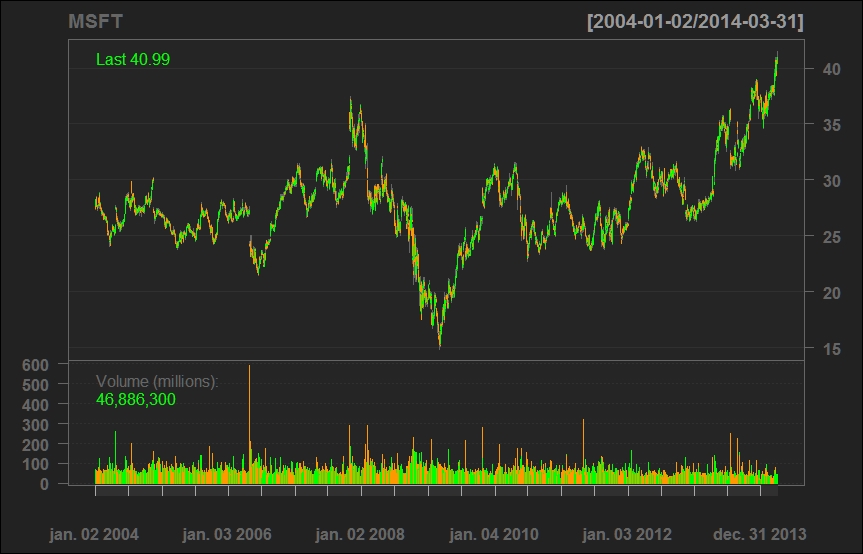
Equity return: This specifies the Microsoft price index from January 01, 2004 to March 03, 2014
Stock index: This specifies the S&P500 index from January 01, 2004 to March 03, 2014
US Treasury bond interest rates from January 01, 2004 to March 03, 2014
Our primary purpose is to make a forecast for the stock market index by using the additional variables and to identify impulse responses. Here, we suppose that there exists a hidden long term relationship between a given stock, the stock market as a whole, and the bond market. The example was chosen primarily to demonstrate several of the data manipulation possibilities of the R programming environment and to illustrate an elaborate concept using a very simple example, and not because of its economic meaning.
We use the vars and quantmod packages. Do not forget to install and load those packages if you haven't done this yet:
install.packages('vars');library('vars')
install.packages('quantmod');library('quantmod')
The Quantmod package offers a great variety of tools to obtain financial data directly from online sources, which we will frequently rely on throughout the book. We use the getSymbols()function:
getSymbols('MSFT', from='2004-01-02', to='2014-03-31')
getSymbols('SNP', from='2004-01-02', to='2014-03-31')
getSymbols('DTB3', src='FRED')
By default, yahoofinance is used as a data source for equity and index price series (src='yahoo' parameter settings, which are omitted in the example). The routine downloads open, high, low, close prices, trading volume, and adjusted prices. The downloaded data is stored in an xts data class, which is automatically named by default after the ticker (MSFT and SNP). It's possible to plot the closing prices by calling the generic plot function, but the chartSeries function of quantmod provides a much better graphical illustration.
The components of the downloaded data can be reached by using the following shortcuts:
Cl(MSFT)     #closing prices
Op(MSFT)     #open prices
Hi(MSFT)     #daily highest price
Lo(MSFT)     #daily lowest price
ClCl(MSFT)   #close-to-close daily return
Ad(MSFT)     #daily adjusted closing price
Thus, for example, by using these shortcuts, the daily close-to-close returns can be plotted as follows:
chartSeries(ClCl(MSFT)) #a plotting example with shortcuts
The screenshot for the preceding command is as follows:
Interest rates are downloaded from the FRED (Federal Reserve Economic Data) data source. The current version of the interface does not allow subsetting of dates; however, downloaded data is stored in an xts data class, which is straightforward to subset to obtain our period of interest:
DTB3.sub <- DTB3['2004-01-02/2014-03-31']
The downloaded prices (which are supposed to be nonstationary series) should be transformed into a stationary series for analysis; that is, we will work with log returns, calculated from the adjusted series:
MSFT.ret <- diff(log(Ad(MSFT)))
SNP.ret  <- diff(log(Ad(SNP)))
To proceed, we need a last data-cleansing step before turning to VAR model fitting. By eyeballing the data, we can see that missing data exists in T-Bill return series, and the lengths of our databases are not the same (on some dates, there are interest rate quotes, but equity prices are missing). To solve these data-quality problems, we choose, for now, the easiest possible solution: merge the databases (by omitting all data points for which we do not have all three data), and omit all NA data. The former is performed by the inner join parameter (see help of the merge function for details):
dataDaily <- na.omit(merge(SNP.ret,MSFT.ret,DTB3.sub), join='inner')
Here, we note that VAR modeling is usually done on lower frequency data. There is a simple way of transforming your data to monthly or quarterly frequencies, by using the following functions, which return with the opening, highest, lowest, and closing value within the given period:
SNP.M  <- to.monthly(SNP.ret)$SNP.ret.Close
MSFT.M <- to.monthly(MSFT.ret)$MSFT.ret.Close
DTB3.M <- to.monthly(DTB3.sub)$DTB3.sub.Close
A simple reduced VAR model may be fitted to the data by using the VAR() function of the vars package. The parameterization shown in the following code allows a maximum of 4 lags in the equations, and choose the model with the best (lowest) Akaike Information Criterion value:
var1 <- VAR(dataDaily, lag.max=4, ic="AIC")
For a more established model selection, you can consider using VARselect(), which provides multiple information criteria (output omitted):
>VARselect(dataDaily,lag.max=4)
The resulting object is an object of the varest class. Estimated parameters and multiple other statistical results can be obtained by the summary() method or the show() method (that is, by just typing the variable):
summary(var1)
var1
There are other methods worth mentioning. The custom plotting method for the varest class generates a diagram for all variables separately, including its fitted values, residuals, and autocorrelation and partial autocorrelation functions of the residuals. You need to hit Enter to get the new variable. Plenty of custom settings are available; please consult the vars package documentation:
plot(var1)       #Diagram of fit and residuals for each variables
coef(var1)       #concise summary of the estimated variables
residuals(var1)  #list of residuals (of the corresponding ~lm)
fitted(var1)     #list of fitted values
Phi(var1)        #coefficient matrices of VMA representation
Predictions using our estimated VAR model can be made by simply calling the predict function and by adding a desired confidence interval:
var.pred <- predict(var1, n.ahead=10, ci=0.95)
Impulse responses should be first generated numerically by irf(), and then they can be plotted by the plot() method. Again, we get different diagrams for each variable, including the respective impulse response functions with bootstrapped confidence intervals as shown in the following command:
var.irf <- irf(var1)
plot(var.irf)
Now, consider fitting a structural VAR model using parameter restrictions described earlier as an A-model. The number of required restrictions for the SVAR model that is identified is  ; in our case, this is 3.
Tip
See Lütkepohl (2007) for more details. The number of additional restrictions required is  , but the diagonal elements are normalized to unity, which leaves us with the preceding number.
The point of departure for an SVAR model is the already estimated reduced form of the VAR model (var1). This has to be amended with an appropriately structured restriction matrix.
For the sake of simplicity, we will use the following restrictions:
S&P index shocks do not have a contemporaneous effect on Microsoft
S&P index shocks do not have a contemporaneous effect on interest rates
T-Bonds interest rate shocks have no contemporaneous effect on Microsoft
These restrictions enter into the SVAR model as 0s in the A matrix, which is as follows:
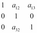
When setting up the A matrix as a parameter for SVAR estimation in R, the positions of the to-be estimated parameters should take the NA value. This can be done with the following assignments:
amat <- diag(3)
amat[2, 1] <- NA
amat[2, 3] <- NA
amat[3, 1] <- NA
Finally, we can fit the SVAR model and plot the impulse response functions (the output is omitted):
svar1 <- SVAR(var1, estmethod='direct', Amat = amat)
irf.svar1 <- irf(svar1)
plot(irf.svar1)
Finally, we put together what we have learned so far, and discuss the concepts of Cointegrated VAR and Vector Error Correction Models (VECM).
Our starting point is a system of cointegrated variables (for example, in a trading context, this indicates a set of similar stocks that are likely to be driven by the same fundamentals). The standard VAR models discussed earlier can only be estimated when the variables are stationary. As we know, the conventional way to remove unit root model is to first differentiate the series; however, in the case of cointegrated series, this would lead to overdifferencing and losing information conveyed by the long-term comovement of variable levels. Ultimately, our goal is to build up a model of stationary variables, which also incorporates the long-term relationship between the original cointegrating nonstationary variables, that is, to build a cointegrated VAR model. This idea is captured by the Vector Error Correction Model (VECM), which consists of a VAR model of the order p - 1 on the differences of the variables, and an error-correction term derived from the known (estimated) cointegrating relationship. Intuitively, and using the stock market example, a VECM model establishes a short-term relationship between the stock returns, while correcting with the deviation from the long-term comovement of prices.
Formally, a two-variable VECM, which we will discuss as a numerical example, can be written as follows. Let  be a vector of two nonstationary unit root series
  where the two series are cointegrated with a cointegrating vector
  . Then, an appropriate VECM model can be formulated as follows:

Here,  and the first term are usually called the error correction terms.
In practice, there are two approaches to test cointegration and build the error correction model. For the two-variable case, the Engle-Granger method is quite instructive; our numerical example basically follows that idea. For the multivariate case, where the maximum number of possible cointegrating relationships is  , you have to follow the Johansen procedure. Although the theoretical framework for the latter goes far beyond the scope of this book, we briefly demonstrate the tools for practical implementation and give references for further studies.
To demonstrate some basic R capabilities regarding VECM models, we will use a standard example of three months and six months T-Bill secondary market rates, which can be downloaded from the FRED database, just as we discussed earlier. We will restrict our attention to an arbitrarily chosen period, that is, from 1984 to 2014. Augmented Dickey Fuller tests indicate that the null hypothesis of the unit root cannot be rejected.
library('quantmod')
getSymbols('DTB3', src='FRED')
getSymbols('DTB6', src='FRED')
DTB3.sub = DTB3['1984-01-02/2014-03-31']
DTB6.sub = DTB6['1984-01-02/2014-03-31']
plot(DTB3.sub)
lines(DTB6.sub, col='red')
We can consistently estimate the cointegrating relationship between the two series by running a simple linear regression. To simplify coding, we define the variables x1 and x2 for the two series, and y for the respective vector series. The other variable-naming conventions in the code snippets will be self-explanatory:
x1=as.numeric(na.omit(DTB3.sub))
x2=as.numeric(na.omit(DTB6.sub))
y = cbind(x1,x2)
cregr <- lm(x1 ~ x2)
r = cregr$residuals
The two series are indeed cointegrated if the residuals of the regression (variable r), that is, the appropriate linear combination of the variables, constitute a stationary series. You could test this with the usual ADF test, but in these settings, the conventional critical values are not appropriate, and corrected values should be used (see, for example Phillips and Ouliaris (1990)).
It is therefore much more appropriate to use a designated test for the existence of cointegration, for example, the Phillips and Ouliaris test, which is implemented in the tseries and in the urca packages as well. The most basic tseries version is demonstrated as follows:
install.packages('tseries');library('tseries');
po.coint <- po.test(y, demean = TRUE, lshort = TRUE)
The null hypothesis states that the two series are not cointegrated, so the low p value indicates rejection of null and presence of cointegration.
The Johansen procedure is applicable for more than one possible cointegrating relationship; an implementation can be found in the urca package:
yJoTest = ca.jo(y, type = c("trace"), ecdet = c("none"), K = 2)

######################
# Johansen-Procedure #
######################

Test type: trace statistic , with linear trend

Eigenvalues (lambda):
[1] 0.0160370678 0.0002322808

Values of teststatistic and critical values of test:

           test 10pct  5pct  1pct
r <= 1 |   1.76  6.50  8.18 11.65
r = 0  | 124.00 15.66 17.95 23.52

Eigenvectors, normalised to first column:
(These are the cointegration relations)

          DTB3.l2   DTB6.l2
DTB3.l2  1.000000  1.000000
DTB6.l2 -0.994407 -7.867356
Weights W:
(This is the loading matrix)

            DTB3.l2      DTB6.l2
DTB3.d -0.037015853 3.079745e-05
DTB6.d -0.007297126 4.138248e-05
The test statistic for r = 0 (no cointegrating relationship) is larger than the critical values, which indicates the rejection of the null. For  , however, the null cannot be rejected; therefore, we conclude that one cointegrating relationship exists. The cointegrating vector is given by the first column of the normalized eigenvectors below the test results.
The final step is to obtain the VECM representation of this system, that is, to run an OLS regression on the lagged differenced variables and the error correction term derived from the previously calculated cointegrating relationship. The appropriate function utilizes the ca.jo object class, which we created earlier. The r = 1 parameter signifies the cointegration rank which is as follows:
>yJoRegr = cajorls(dyTest, r=1)
>yJoRegr

$rlm

Call:
lm(formula = substitute(form1), data = data.mat)

Coefficients:
          x1.d        x2.d
ect1      -0.0370159  -0.0072971
constant  -0.0041984  -0.0016892
x1.dl1     0.1277872   0.1538121
x2.dl1     0.0006551  -0.0390444

$beta
           ect1
x1.l1  1.000000
x2.l1 -0.994407
The coefficient of the error-correction term is negative, as we expected; a short-term deviation from the long-term equilibrium level would push our variables back to the zero equilibrium deviation.
You can easily check this in the bivariate case; the result of the Johansen procedure method leads to approximately the same result as the step-by-step implementation of the ECM following the Engle-Granger procedure. This is shown in the uploaded R code files.
It is a well-known and commonly accepted stylized fact in empirical finance that the volatility of financial time series varies over time. However, the non-observable nature of volatility makes the measurement and forecasting a challenging exercise. Usually, varying volatility models are motivated by three empirical observations:
Volatility clustering: This refers to the empirical observation that calm periods are usually followed by calm periods while turbulent periods by turbulent periods in the financial markets.
Non-normality of asset returns: Empirical analysis has shown that asset returns tend to have fat tails relative to the normal distribution.
Leverage effect: This leads to an observation that volatility tends to react differently to positive or negative price movements; a drop in prices increases the volatility to a larger extent than an increase of similar size.
In the following code, we demonstrate these stylized facts based on S&P asset prices. Data is downloaded from yahoofinance, by using the already known method:
getSymbols("SNP", from="2004-01-01", to=Sys.Date())
chartSeries(Cl(SNP))
Our purpose of interest is the daily return series, so we calculate log returns from the closing prices. Although it is a straightforward calculation, the Quantmod package offers an even simpler way:
ret <- dailyReturn(Cl(SNP), type='log')
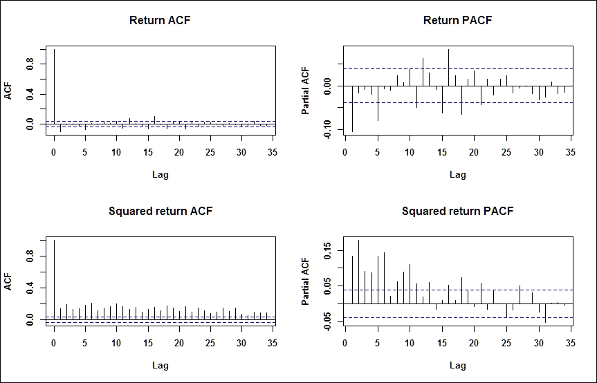
Volatility analysis departs from eyeballing the autocorrelation and partial autocorrelation functions. We expect the log returns to be serially uncorrelated, but the squared or absolute log returns to show significant autocorrelations. This means that Log returns are not correlated, but not independent.
Notice the par(mfrow=c(2,2)) function in the following code; by this, we overwrite the default plotting parameters of R to organize the four diagrams of interest in a convenient table format:
par(mfrow=c(2,2))
acf(ret, main="Return ACF");
pacf(ret, main="Return PACF");
acf(ret^2, main="Squared return ACF");
pacf(ret^2, main="Squared return PACF")
par(mfrow=c(1,1))
The screenshot for preceding command is as follows:
Next, we look at the histogram and/or the empirical distribution of daily log returns of S&P and compare it with the normal distribution of the same mean and standard deviation. For the latter, we use the function density(ret), which computes the nonparametric empirical distribution function. We use the function curve()with an additional parameter add=TRUE to plot a second line to an already existing diagram:
m=mean(ret);s=sd(ret);
par(mfrow=c(1,2))
hist(ret, nclass=40, freq=FALSE, main='Return histogram');curve(dnorm(x, mean=m,sd=s), from = -0.3, to = 0.2, add=TRUE, col="red")
plot(density(ret), main='Return empirical distribution');curve(dnorm(x, mean=m,sd=s), from = -0.3, to = 0.2, add=TRUE, col="red")
par(mfrow=c(1,1))
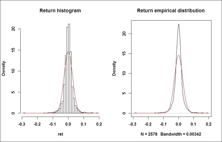
The excess kurtosis and fat tails are obvious, but we can confirm numerically (using the moments package) that the kurtosis of the empirical distribution of our sample exceeds that of a normal distribution (which is equal to 3). Unlike some other software packages, R reports the nominal value of kurtosis, and not excess kurtosis which is as follows:
> kurtosis(ret)
daily.returns
     12.64959
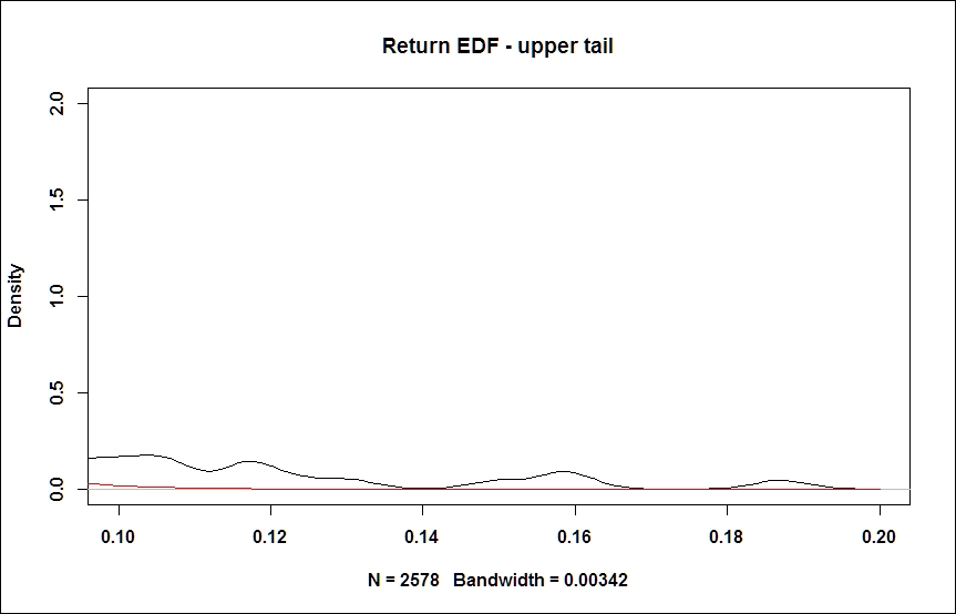
It might be also useful to zoom in to the upper or the lower tail of the diagram. This is achieved by simply rescaling our diagrams:
# tail zoom
plot(density(ret), main='Return EDF - upper tail', xlim = c(0.1, 0.2), ylim=c(0,2));
curve(dnorm(x, mean=m,sd=s), from = -0.3, to = 0.2, add=TRUE, col="red")
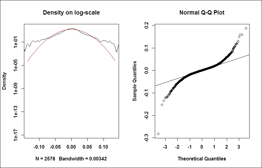
Another useful visualization exercise is to look at the Density on log-scale (see the following figure, left), or a QQ-plot (right), which are common tools to comparing densities. QQ-plot depicts the empirical quantiles against that of a theoretical (normal) distribution. In case our sample is taken from a normal distribution, this should form a straight line. Deviations from this straight line may indicate the presence of fat tails:
# density plots on log-scale
plot(density(ret), xlim=c(-5*s,5*s),log='y', main='Density on log-scale')
curve(dnorm(x, mean=m,sd=s), from=-5*s, to=5*s, log="y", add=TRUE, col="red")

# QQ-plot
qqnorm(ret);qqline(ret);
The screenshot for preceding command is as follows:
Now, we can turn our attention to modeling volatility.
Broadly speaking, there are two types of modeling techniques in the financial econometrics literature to capture the varying nature of volatility: the GARCH-family approach (Engle, 1982 and Bollerslev, 1986) and the stochastic volatility (SV) models. As for the distinction between them, the main difference between the GARCH-type modeling and (genuine) SV-type modeling techniques is that in the former, the conditional variance given in the past observations is available, while in SV-models, volatility is not measurable with respect to the available information set; therefore, it is hidden by nature, and must be filtered out from the measurement equation (see, for example, Andersen – Benzoni (2011)). In other words, GARCH-type models involve the estimation of volatility based on past observations, while in SV-models, the volatility has its own stochastic process, which is hidden, and return realizations should be used as a measurement equation to make inferences regarding the underlying volatility process.
In this chapter, we introduce the basic modeling techniques for the GARCH approach for two reasons; first of all, it is much more proliferated in applied works. Secondly, because of its diverse methodological background, SV models are not yet supported by R packages natively, and a significant amount of custom development is required for an empirical implementation.
There are several packages available in R for GARCH modeling. The most prominent ones are rugarch, rmgarch (for multivariate models), and fGarch; however, the basic tseries package also includes some GARCH functionalities. In this chapter, we will demonstrate the modeling facilities of the rugarch package. Our notations in this chapter follow the respective ones of the rugarch package's output and documentation.
A GARCH (p,q) process may be written as follows:

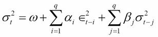
Here,  is usually the disturbance term of a conditional mean equation (in practice, usually an ARMA process) and
  . That is, the conditional volatility process is determined linearly by its own lagged values
  and the lagged squared observations (the values of ). In empirical studies, GARCH (1,1) usually provides an appropriate fit to the data. It may be useful to think about the simple GARCH (1,1) specification as a model in which the conditional variance is specified as a weighted average of the long-run variance
  , the last predicted variance
  , and the new information
  (see Andersen et al. (2009)). It is easy to see how the GARCH (1,1) model captures autoregression in volatility (volatility clustering) and leptokurtic asset return distributions, but as its main drawback, it is symmetric, and cannot capture asymmetries in distributions and leverage effects.
The emergence of volatility clustering in a GARCH-model is highly intuitive; a large positive (negative) shock in  increases (decreases) the value of , which in turn increases (decreases) the value of
  , resulting in a larger (smaller) value for
  . The shock is persistent; this is volatility clustering. Leptokurtic nature requires some derivation; see for example Tsay (2010).
Our empirical example will be the analysis of the return series calculated from the daily closing prices of Apple Inc. based on the period from Jan 01, 2006 to March 31, 2014. As a useful exercise, before starting this analysis, we recommend that you repeat the exploratory data analysis in this chapter to identify stylized facts on Apple data.
Obviously, our first step is to install a package, if not installed yet:
install.packages('rugarch');library('rugarch')
To get the data, as usual, we use the quantmod package and the getSymbols() function, and calculate return series based on the closing prices.
#Load Apple data and calculate log-returns
getSymbols("AAPL", from="2006-01-01", to="2014-03-31")
ret.aapl <- dailyReturn(Cl(AAPL), type='log')
chartSeries(ret.aapl)
The programming logic of rugarch can be thought of as follows: irrespective of whatever your aim is (fitting, filtering, forecasting, and simulating), first, you have to specify a model as a system object (variable), which in turn will be inserted into the respective function. Models can be specified by calling ugarchspec(). The following code specifies a simple GARCH (1,1) model, (sGARCH), with only a constant  in the mean equation:
garch11.spec = ugarchspec(variance.model = list(model="sGARCH", garchOrder=c(1,1)), mean.model = list(armaOrder=c(0,0)))
An obvious way to proceed is to fit this model to our data, that is, to estimate the unknown parameters by maximum likelihood, based on our time series of daily returns:
aapl.garch11.fit = ugarchfit(spec=garch11.spec, data=ret.aapl)
The function provides, among a number of other outputs, the parameter estimations  :
:
> coef(aapl.garch11.fit)
          mu        omega       alpha1        beta1
1.923328e-03 1.027753e-05 8.191681e-02 8.987108e-01
Estimates and various diagnostic tests can be obtained by the show() method of the generated object (that is, by just typing the name of the variable). A bunch of other statistics, parameter estimates, standard error, and covariance matrix estimates can be reached by typing the appropriate command. For the full list, consult the ugarchfit object class; the most important ones are shown in the following code:
coef(msft.garch11.fit)          #estimated coefficients
vcov(msft.garch11.fit)          #covariance matrix of param estimates
infocriteria(msft.garch11.fit)  #common information criteria list
newsimpact(msft.garch11.fit)    #calculate news impact curve
signbias(msft.garch11.fit)      #Engle - Ng sign bias test
fitted(msft.garch11.fit)        #obtain the fitted data series
residuals(msft.garch11.fit)     #obtain the residuals
uncvariance(msft.garch11.fit)   #unconditional (long-run) variance
uncmean(msft.garch11.fit)       #unconditional (long-run) mean
Standard GARCH models are able to capture fat tails and volatility clustering, but to explain asymmetries caused by the leverage effect, we need more advanced models. To approach the asymmetry problem visually, we will now describe the concept of news impact curves.
News impact curves, introduced by Pagan and Schwert (1990) and Engle and Ng (1991), are useful tools to visualize the magnitude of volatility changes in response to shocks. The name comes from the usual interpretation of shocks as news influencing the market movements. They plot the change in conditional volatility against shocks in different sizes, and can concisely express the asymmetric effects in volatility. In the following code, the first line calculates the news impacts numerically for the previously defined GARCH(1,1) model, and the second line creates the visual plot:
ni.garch11 <- newsimpact(aapl.garch11.fit)
plot(ni.garch11$zx, ni.garch11$zy, type="l", lwd=2, col="blue", main="GARCH(1,1) - News Impact", ylab=ni.garch11$yexpr, xlab=ni.garch11$xexpr)
The screenshot for the preceding command is as follows:
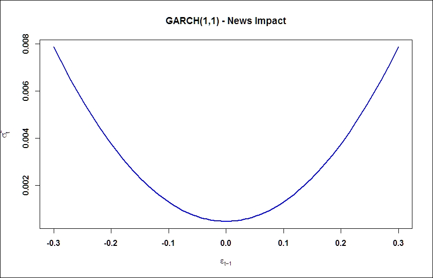
As we expected, no asymmetries are present in response to positive and negative shocks. Now, we turn to models to be able to incorporate asymmetric effects as well.
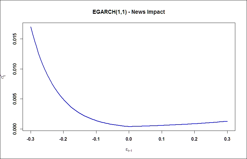
Exponential GARCH models were introduced by Nelson (1991). This approach directly models the logarithm of the conditional volatility:
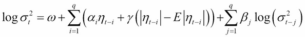
where, E is the expectation operator. This model formulation allows multiplicative dynamics in evolving the volatility process. Asymmetry is captured by the  parameter; a negative value indicates that the process reacts more to negative shocks, as observable in real data sets.
To fit an EGARCH model, the only parameter to be changed in a model specification is to set the EGARCH model type. By running the fitting function, the additional parameter will be estimated (see coef()):
# specify EGARCH(1,1) model with only constant in mean equation
egarch11.spec = ugarchspec(variance.model = list(model="eGARCH", garchOrder=c(1,1)), mean.model = list(armaOrder=c(0,0)))
aapl.egarch11.fit = ugarchfit(spec=egarch11.spec, data=ret.aapl)

> coef(aapl.egarch11.fit)
          mu        omega       alpha1        beta1       gamma1
 0.001446685 -0.291271433 -0.092855672  0.961968640  0.176796061
News impact curve reflects the strong asymmetry in response of conditional volatility to shocks and confirms the necessity of asymmetric models:
ni.egarch11 <- newsimpact(aapl.egarch11.fit)
plot(ni.egarch11$zx, ni.egarch11$zy, type="l", lwd=2, col="blue", main="EGARCH(1,1) - News Impact",
ylab=ni.egarch11$yexpr, xlab=ni.egarch11$xexpr)
Another prominent example is the TGARCH model, which is even easier to interpret. The TGARCH specification involves an explicit distinction of model parameters above and below a certain threshold. TGARCH is also a submodel of a more general class, the asymmetric power ARCH class, but we will discuss it separately because of its wide penetration in applied financial econometrics literature.
The TGARCH model may be formulated as follows:
where 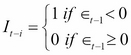
The interpretation is straightforward; the ARCH coefficient depends on the sign of the previous error term; if  is positive, a negative error term will have a higher impact on the conditional volatility, just as we have seen in the leverage effect before.
In the R package, rugarch, the threshold GARCH model is implemented in a framework of an even more general class of GARCH models, called the Family GARCH model Ghalanos (2014).
# specify TGARCH(1,1) model with only constant in mean equation
tgarch11.spec = ugarchspec(variance.model = list(model="fGARCH", submodel="TGARCH", garchOrder=c(1,1)),
          mean.model = list(armaOrder=c(0,0)))
aapl.tgarch11.fit = ugarchfit(spec=tgarch11.spec, data=ret.aapl)

> coef(aapl.egarch11.fit)
          mu        omega       alpha1        beta1       gamma1
 0.001446685 -0.291271433 -0.092855672  0.961968640  0.176796061
Thanks to the specific functional form, the news impact curve for a Threshold-GARCH is less flexible in representing different responses, there is a kink at the zero point which can be seen when we run the following command:
ni.tgarch11 <- newsimpact(aapl.tgarch11.fit)
plot(ni.tgarch11$zx, ni.tgarch11$zy, type="l", lwd=2, col="blue", main="TGARCH(1,1) - News Impact",
ylab=ni.tgarch11$yexpr, xlab=ni.tgarch11$xexpr)
The Rugarch package allows an easy way to simulate from a specified model. Of course, for simulation purposes, we should also specify the parameters of the model within ugarchspec(); this could be done by the fixed.pars argument. After specifying the model, we can simulate a time series with a given conditional mean and GARCH specification by using simply the ugarchpath() function:
garch11.spec = ugarchspec(variance.model = list(garchOrder=c(1,1)),
  mean.model = list(armaOrder=c(0,0)),
    fixed.pars=list(mu = 0, omega=0.1, alpha1=0.1,
      beta1 = 0.7))
garch11.sim = ugarchpath(garch11.spec, n.sim=1000)
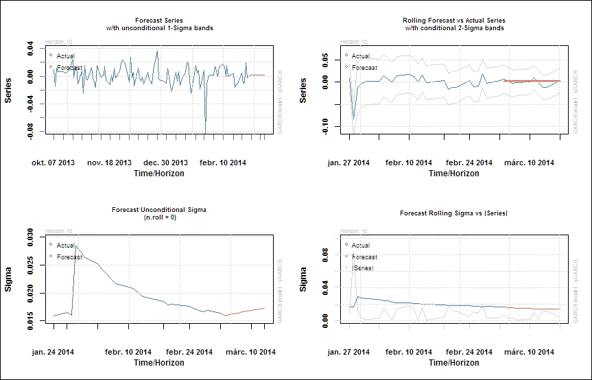
Once we have an estimated model and technically a fitted object, forecasting the conditional volatility based on that is just one step:
aapl.garch11.fit = ugarchfit(spec=garch11.spec, data=ret.aapl, out.sample=20)
aapl.garch11.fcst = ugarchforecast(aapl.garch11.fit, n.ahead=10, n.roll=10)
The plotting method of the forecasted series provides the user with a selection menu; we can plot either the predicted time series or the predicted conditional volatility.
plot(aapl.garch11.fcst, which='all')
In this chapter, we reviewed some important concepts of time series analysis, such as cointegration, vector-autoregression, and GARCH-type conditional volatility models. Meanwhile, we have provided a useful introduction to some tips and tricks to start modeling with R for quantitative and empirical finance. We hope that you find these exercises useful, but again, it should be noted that this chapter is far from being complete both from time series and econometric theory, and from R programming's point of view. The R programming language is very well documented on the Internet, and the R user's community consists of thousands of advanced and professional users. We encourage you to go beyond books, be a self-learner, and do not stop if you are stuck with a problem; almost certainly, you will find an answer on the Internet to proceed. Use the documentation of R packages and the help files heavily, and study the official R-site, http://cran.r-project.org/, frequently. The remaining chapters will provide you with numerous additional examples to find your way in the plethora of R facilities, packages, and functions.
Andersen, Torben G; Davis, Richard A.; Kreiß, Jens-Peters; Mikosh, Thomas (ed.) (2009). Handbook of Financial Time Series
Andersen, Torben G. and Benzoni, Luca (2011). Stochastic volatility. Book chapter in Complex Systems in Finance and Econometrics, Ed.: Meyers, Robert A., Springer
Brooks, Chris (2008). Introductory Econometrics for Finance, Cambridge University Press
Fry, Renee and Pagan, Adrian (2011). Sign Restrictions in Structural Vector Autoregressions: A Critical Review. Journal of Economic Literature, American Economic Association, vol. 49(4), pages 938-60, December.
Ghalanos, Alexios (2014) Introduction to the rugarch package http://cran.r-project.org/web/packages/rugarch/vignettes/Introduction_to_the_rugarch_package.pdf
Hafner, Christian M. (2011). Garch modelling. Book chapter in Complex Systems in Finance and Econometrics, Ed.: Meyers, Robert A., Springer
Hamilton, James D. (1994). Time Series Analysis, Princetown, New Jersey
Lütkepohl, Helmut (2007). New Introduction to Multiple Time Series Analysis, Springer
Murray, Michael. P. (1994). A drunk and her dog: an illustration of cointegration and error correction. The American Statistician, 48(1), 37-39.
Martin, Vance; Hurn, Stan and Harris, David (2013). Econometric Modelling with Time Series. Specification, Estimation and Testing, Cambridge University Press
Pfaff, Bernard (2008). Analysis of Integrated and Cointegrated Time Series with R, Springer
Pfaff, Bernhard (2008). VAR, SVAR and SVEC Models: Implementation Within R Package vars. Journal of Statistical Software, 27(4)
Phillips, P. C., & Ouliaris, S. (1990). Asymptotic properties of residual based tests for cointegration. Econometrica: Journal of the Econometric Society, 165-193.
Pole, Andrew (2007). Statistical Arbitrage. Wiley
Rachev, Svetlozar T., Hsu, John S.J., Bagasheva, Biliana S. and Fabozzi, Frank J. (2008). Bayesian Methods in Finance. John Wiley & Sons.
Sims, Christopher A. (1980). Macroeconomics and reality. Econometrica: Journal of the Econometric Society, 1-48.
Tsay, Ruey S. (2010). Analysis of Financial Time Series, 3rd edition, Wiley