


A graphical model is essentially a way of representing joint probability distribution over a set of random variables in a compact and intuitive form. There are two main types of graphical models, namely directed and undirected. We generally use a directed model, also known as a Bayesian network, when we mostly have a causal relationship between the random variables. Graphical models also give us tools to operate on these models to find conditional and marginal probabilities of variables, while keeping the computational complexity under control.
In this chapter, we will cover:
The basics of random variables, probability theory, and graph theory
Bayesian models
Independencies in Bayesian models
The relation between graph structure and probability distribution in Bayesian networks (IMAP)
Different ways of representing a conditional probability distribution
Code examples for all of these using
pgmpy
To understand the concepts of probability theory, let's start with a real-life situation. Let's assume we want to go for an outing on a weekend. There are a lot of things to consider before going: the weather conditions, the traffic, and many other factors. If the weather is windy or cloudy, then it is probably not a good idea to go out. However, even if we have information about the weather, we cannot be completely sure whether to go or not; hence we have used the words probably or maybe. Similarly, if it is windy in the morning (or at the time we took our observations), we cannot be completely certain that it will be windy throughout the day. The same holds for cloudy weather; it might turn out to be a very pleasant day. Further, we are not completely certain of our observations. There are always some limitations in our ability to observe; sometimes, these observations could even be noisy. In short, uncertainty or randomness is the innate nature of the world. The probability theory provides us the necessary tools to study this uncertainty. It helps us look into options that are unlikely yet probable.
Probability deals with the study of events. From our intuition, we can say that some events are more likely than others, but to quantify the likeliness of a particular event, we require the probability theory. It helps us predict the future by assessing how likely the outcomes are.
Before going deeper into the probability theory, let's first get acquainted with the basic terminologies and definitions of the probability theory. A random variable is a way of representing an attribute of the outcome. Formally, a random variable X is a function that maps a possible set of outcomes Ω to some set E, which is represented as follows:
X : Ω → E
As an example, let us consider the outing example again. To decide whether to go or not, we may consider the skycover (to check whether it is cloudy or not). Skycover is an attribute of the day. Mathematically, the random variable skycover (X) is interpreted as a function, which maps the day (Ω) to its skycover values (E). So when we say the event X = 40.1, it represents the set of all the days {ω} such that  , where
  is the mapping function. Formally speaking,
  .
.
Random variables can either be discrete or continuous. A discrete random variable can only take a finite number of values. For example, the random variable representing the outcome of a coin toss can take only two values, heads or tails; and hence, it is discrete. Whereas, a continuous random variable can take infinite number of values. For example, a variable representing the speed of a car can take any number values.
For any event whose outcome is represented by some random variable (X), we can assign some value to each of the possible outcomes of X, which represents how probable it is. This is known as the probability distribution of the random variable and is denoted by P(X).
For example, consider a set of restaurants. Let X be a random variable representing the quality of food in a restaurant. It can take up a set of values, such as {good, bad, average}. P(X), represents the probability distribution of X, that is, if P(X = good) = 0.3, P(X = average) = 0.5, and P(X = bad) = 0.2. This means there is 30 percent chance of a restaurant serving good food, 50 percent chance of it serving average food, and 20 percent chance of it serving bad food.
In most of the situations, we are rather more interested in looking at multiple attributes at the same time. For example, to choose a restaurant, we won't only be looking just at the quality of food; we might also want to look at other attributes, such as the cost, location, size, and so on. We can have a probability distribution over a combination of these attributes as well. This type of distribution is known as joint probability distribution. Going back to our restaurant example, let the random variable for the quality of food be represented by Q, and the cost of food be represented by C. Q can have three categorical values, namely {good, average, bad}, and C can have the values {high, low}. So, the joint distribution for P(Q, C) would have probability values for all the combinations of states of Q and C. P(Q = good, C = high) will represent the probability of a pricey restaurant with good quality food, while P(Q = bad, C = low) will represent the probability of a restaurant that is less expensive with bad quality food.
Let us consider another random variable representing an attribute of a restaurant, its location L. The cost of food in a restaurant is not only affected by the quality of food but also the location (generally, a restaurant located in a very good location would be more costly as compared to a restaurant present in a not-very-good location). From our intuition, we can say that the probability of a costly restaurant located at a very good location in a city would be different (generally, more) than simply the probability of a costly restaurant, or the probability of a cheap restaurant located at a prime location of city is different (generally less) than simply probability of a cheap restaurant. Formally speaking, P(C = high | L = good) will be different from P(C = high) and P(C = low | L = good) will be different from P(C = low). This indicates that the random variables C and L are not independent of each other.
These attributes or random variables need not always be dependent on each other. For example, the quality of food doesn't depend upon the location of restaurant. So, P(Q = good | L = good) or P(Q = good | L = bad)would be the same as P(Q = good), that is, our estimate of the quality of food of the restaurant will not change even if we have knowledge of its location. Hence, these random variables are independent of each other.
In general, random variables  can be considered as independent of each other, if:

They may also be considered independent if:
We can easily derive this conclusion. We know the following from the chain rule of probability:
P(X, Y) = P(X) P(Y | X)
If Y is independent of X, that is, if X | Y, then P(Y | X) = P(Y). Then:
P(X, Y) = P(X) P(Y)
Extending this result on multiple variables, we can easily get to the conclusion that a set of random variables are independent of each other, if their joint probability distribution is equal to the product of probabilities of each individual random variable.
Sometimes, the variables might not be independent of each other. To make this clearer, let's add another random variable, that is, the number of people visiting the restaurant N. Let's assume that, from our experience we know the number of people visiting only depends on the cost of food at the restaurant and its location (generally, lesser number of people visit costly restaurants). Does the quality of food Q affect the number of people visiting the restaurant? To answer this question, let's look into the random variable affecting N, cost C, and location L. As C is directly affected by Q, we can conclude that Q affects N. However, let's consider a situation when we know that the restaurant is costly, that is, C = high and let's ask the same question, "does the quality of food affect the number of people coming to the restaurant?". The answer is no. The number of people coming only depends on the price and location, so if we know that the cost is high, then we can easily conclude that fewer people will visit, irrespective of the quality of food. Hence,  .
.
This type of independence is called conditional independence.
Let's now see some coding examples using pgmpy, to represent joint distributions and independencies. Here, we will mostly work with IPython and pgmpy (and a few other libraries) for coding examples. So, before moving ahead, let's get a basic introduction to these.
IPython is a command shell for interactive computing in multiple programming languages, originally developed for the Python programming language, which offers enhanced introspection, rich media, additional shell syntax, tab completion, and a rich history. IPython provides the following features:
Powerful interactive shells (terminal and Qt-based)
A browser-based notebook with support for code, text, mathematical expressions, inline plots, and other rich media
Support for interactive data visualization and use of GUI toolkits
Flexible and embeddable interpreters to load into one's own projects
Easy-to-use and high performance tools for parallel computing
You can install IPython using the following command:
>>> pip3 install ipython
To start the IPython command shell, you can simply type ipython3 in the terminal. For more installation instructions, you can visit http://ipython.org/install.html.
pgmpy is a Python library to work with Probabilistic Graphical models. As it's currently not on PyPi, we will need to build it manually. You can get the source code from the Git repository using the following command:
>>> git clone https://github.com/pgmpy/pgmpy
Now cd into the cloned directory switch branch for version used in this book and build it with the following code:
>>> cd pgmpy
>>> git checkout book/v0.1
>>> sudo python3 setup.py install
For more installation instructions, you can visit http://pgmpy.org/install.html.
With both IPython and pgmpy installed, you should now be able to run the examples in the book.
To represent independencies, pgmpy has two classes, namely IndependenceAssertion and Independencies. The IndependenceAssertion class is used to represent individual assertions of the form of  or
or  . Let's see some code to represent assertions:
# Firstly we need to import IndependenceAssertion
In [1]: from pgmpy.independencies import IndependenceAssertion
# Each assertion is in the form of [X, Y, Z] meaning X is
# independent of Y given Z.
In [2]: assertion1 = IndependenceAssertion('X', 'Y')
In [3]: assertion1
Out[3]: (X _|_ Y)
Here, assertion1 represents that the variable X is independent of the variable Y. To represent conditional assertions, we just need to add a third argument to IndependenceAssertion:
In  [4]: assertion2 = IndependenceAssertion('X', 'Y', 'Z')
In  [5]: assertion2
Out [5]: (X _|_ Y | Z)
In the preceding example, assertion2 represents .
IndependenceAssertion also allows us to represent assertions in the form of  . To do this, we just need to pass a list of random variables as arguments:
In [4]: assertion2 = IndependenceAssertion('X', 'Y', 'Z')
In [5]: assertion2
Out[5]: (X _|_ Y | Z)
Moving on to the Independencies class, an Independencies object is used to represent a set of assertions. Often, in the case of Bayesian or Markov networks, we have more than one assertion corresponding to a given model, and to represent these independence assertions for the models, we generally use the Independencies object. Let's take a few examples:
In [8]: from pgmpy.independencies import Independencies
# There are multiple ways to create an Independencies object, we
# could either initialize an empty object or initialize with some
# assertions.

In [9]: independencies = Independencies() # Empty object
In [10]: independencies.get_assertions()
Out[10]: []

In [11]: independencies.add_assertions(assertion1, assertion2)
In [12]: independencies.get_assertions()
Out[12]: [(X _|_ Y), (X _|_ Y | Z)]
We can also directly initialize Independencies in these two ways:
In [13]: independencies = Independencies(assertion1, assertion2)
In [14]: independencies = Independencies(['X', 'Y'],
                                         ['A', 'B', 'C'])
In [15]: independencies.get_assertions()
Out[15]: [(X _|_ Y), (A _|_ B | C)]We can also represent joint probability distributions using pgmpy's JointProbabilityDistribution class. Let's say we want to represent the joint distribution over the outcomes of tossing two fair coins. So, in this case, the probability of all the possible outcomes would be 0.25, which is shown as follows:
In [16]: from pgmpy.factors import JointProbabilityDistribution as Joint
In [17]: distribution = Joint(['coin1', 'coin2'],
                              [2, 2],
                              [0.25, 0.25, 0.25, 0.25])
Here, the first argument includes names of random variable. The second argument is a list of the number of states of each random variable. The third argument is a list of probability values, assuming that the first variable changes its states the slowest. So, the preceding distribution represents the following:
In [18]: print(distribution)
╒═════════╤═════════╤══════════════════╕
│ coin1   │ coin2   │   P(coin1,coin2) │
╞═════════╪═════════╪══════════════════╡
│ coin1_0 │ coin2_0 │   0.2500         │
├─────────┼─────────┼──────────────────┤
│ coin1_0 │ coin2_1 │   0.2500         │
├─────────┼─────────┼──────────────────┤
│ coin1_1 │ coin2_0 │   0.2500         │
├─────────┼─────────┼──────────────────┤
│ coin1_1 │ coin2_1 │   0.2500         │
╘═════════╧═════════╧══════════════════╛
We can also conduct independence queries over these distributions in pgmpy:
In [19]: distribution.check_independence('coin1', 'coin2')
Out[20]: TrueLet's take an example to understand conditional probability better. Let's say we have a bag containing three apples and five oranges, and we want to randomly take out fruits from the bag one at a time without replacing them. Also, the random variables  and
and  represent the outcomes in the first try and second try respectively. So, as there are three apples and five oranges in the bag initially,
  and
and  . Now, let's say that in our first attempt we got an orange. Now, we cannot simply represent the probability of getting an apple or orange in our second attempt. The probabilities in the second attempt will depend on the outcome of our first attempt and therefore, we use conditional probability to represent such cases. Now, in the second attempt, we will have the following probabilities that depend on the outcome of our first try:
 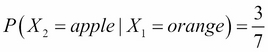 ,
, 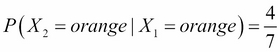 ,
, 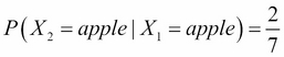 , and
, and 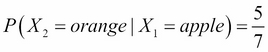 .
.
The Conditional Probability Distribution (CPD) of two variables and can be represented as  , representing the probability of given that is the probability of after the event has occurred and we know it's outcome. Similarly, we can have
  representing the probability of after having an observation for .
The simplest representation of CPD is tabular CPD. In a tabular CPD, we construct a table containing all the possible combinations of different states of the random variables and the probabilities corresponding to these states. Let's consider the earlier restaurant example.
Let's begin by representing the marginal distribution of the quality of food with Q. As we mentioned earlier, it can be categorized into three values {good, bad, average}. For example, P(Q) can be represented in the tabular form as follows:
|
Quality |
P(Q) |
|---|---|
|
Good |
0.3 |
|
Normal |
0.5 |
|
Bad |
0.2 |
Similarly, let's say P(L) is the probability distribution of the location of the restaurant. Its CPD can be represented as follows:
|
Location |
P(L) |
|---|---|
|
Good |
0.6 |
|
Bad |
0.4 |
As the cost of restaurant C depends on both the quality of food Q and its location L, we will be considering P(C | Q, L), which is the conditional distribution of C, given Q and L:
|
Location |
Good |
Bad | ||||
|---|---|---|---|---|---|---|
|
Quality |
Good |
Normal |
Bad |
Good |
Normal |
Bad |
|
Cost | ||||||
|
High |
0.8 |
0.6 |
0.1 |
0.6 |
0.6 |
0.05 |
|
Low |
0.2 |
0.4 |
0.9 |
0.4 |
0.4 |
0.95 |
Let's first see how to represent the tabular CPD using pgmpy for variables that have no conditional variables:
In [1]: from pgmpy.factors import TabularCPD

# For creating a TabularCPD object we need to pass three
# arguments: the variable name, its cardinality that is the number
# of states of the random variable and the probability value
# corresponding each state.
In [2]: quality = TabularCPD(variable='Quality',
                             variable_card=3,
                                values=[[0.3], [0.5], [0.2]])
In [3]: print(quality)
╒════════════════╤═════╕
│ ['Quality', 0] │ 0.3 │
├────────────────┼─────┤
│ ['Quality', 1] │ 0.5 │
├────────────────┼─────┤
│ ['Quality', 2] │ 0.2 │
╘════════════════╧═════╛
In [4]: quality.variables
Out[4]: OrderedDict([('Quality', [State(var='Quality', state=0),
                                  State(var='Quality', state=1),
                                  State(var='Quality', state=2)])])

In [5]: quality.cardinality
Out[5]: array([3])

In [6]: quality.values
Out[6]: array([0.3, 0.5, 0.2])
You can see here that the values of the CPD are a 1D array instead of a 2D array, which you passed as an argument. Actually, pgmpy internally stores the values of the TabularCPD as a flattened numpy array. We will see the reason for this in the next chapter.
In [7]: location = TabularCPD(variable='Location',
                              variable_card=2,
                              values=[[0.6], [0.4]])
In [8]: print(location)
╒═════════════════╤═════╕
│ ['Location', 0] │ 0.6 │
├─────────────────┼─────┤
│ ['Location', 1] │ 0.4 │
╘═════════════════╧═════╛
However, when we have conditional variables, we also need to specify them and the cardinality of those variables. Let's define the TabularCPD for the cost variable:
In [9]: cost = TabularCPD(
                      variable='Cost',
                      variable_card=2,
                      values=[[0.8, 0.6, 0.1, 0.6, 0.6, 0.05],
                              [0.2, 0.4, 0.9, 0.4, 0.4, 0.95]],
                      evidence=['Q', 'L'],
evidence_card=[3, 2])The second major framework for the study of probabilistic graphical models is graph theory. Graphs are the skeleton of PGMs, and are used to compactly encode the independence conditions of a probability distribution.
The foundation of graph theory was laid by Leonhard Euler when he solved the famous Seven Bridges of Konigsberg problem. The city of Konigsberg was set on both sides by the Pregel river and included two islands that were connected and maintained by seven bridges. The problem was to find a walk to exactly cross all the bridges once in a single walk.
To visualize the problem, let's think of the graph in Fig 1.1:
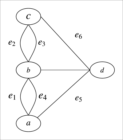
Fig 1.1: The Seven Bridges of Konigsberg graph
Here, the nodes a, b, c, and d represent the land, and are known as vertices of the graph. The line segments ab, bc, cd, da, ab, and bc connecting the land parts are the bridges and are known as the edges of the graph. So, we can think of the problem of crossing all the bridges once in a single walk as tracing along all the edges of the graph without lifting our pencils.
Formally, a graph G = (V, E) is an ordered pair of finite sets. The elements of the set V are known as the nodes or the vertices of the graph, and the elements of  are the edges or the arcs of the graph. The number of nodes or cardinality of G, denoted by |V|, are known as the order of the graph. Similarly, the number of edges denoted by |E| are known as the size of the graph. Here, we can see that the Konigsberg city graph shown in Fig 1.1 is of order 4 and size 7.
In a graph, we say that two vertices, u, v
ϵ
V are adjacent if u, v
ϵ
E. In the City graph, all the four vertices are adjacent to each other because there is an edge for every possible combination of two vertices in the graph. Also, for a vertex v
ϵ
V, we define the neighbors set of v as 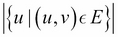 . In the City graph, we can see that b and d are neighbors of c. Similarly, a, b, and c are neighbors of d.
We define an edge to be a self loop if the start vertex and the end vertex of the edge are the same. We can put it more formally as, any edge of the form (u, u), where u ϵ V is a self loop.
Until now, we have been talking only about graphs whose edges don't have a direction associated with them, which means that the edge (u, v) is same as the edge (v, u). These types of graphs are known as undirected graphs. Similarly, we can think of a graph whose edges have a sense of direction associated with it. For these graphs, the edge set E would be a set of ordered pair of vertices. These types of graphs are known as directed graphs. In the case of a directed graph, we also define the indegree and outdegree for a vertex. For a vertex v
ϵ
V, we define its outdegree as the number of edges originating from the vertex v, that is, 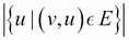 . Similarly, the indegree is defined as the number of edges that end at the vertex v, that is, .
For a graph G = (V, E) and u,v
ϵ
V, we define a u - v walk as an alternating sequence of vertices and edges, starting with u and ending with v. In the City graph of Fig 1.1, we can have an example of a - d walk as 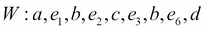 .
.
If there aren't multiple edges between the same vertices, then we simply represent a walk by a sequence of vertices. As in the case of the Butterfly graph shown in Fig 1.2, we can have a walk W : a, c, d, c, e:
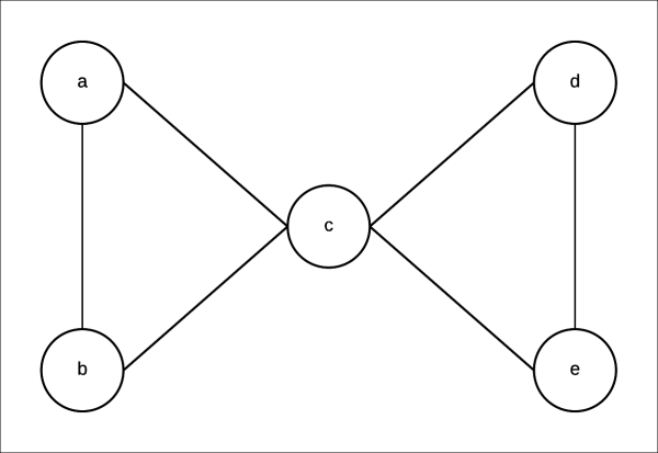
Fig 1.2: Butterfly graph—a undirected graph
A walk with no repeated edges is known as a trail. For example, the walk 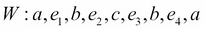 in the City graph is a trail. Also, a walk with no repeated vertices, except possibly the first and the last, is known as a path. For example, the walk
 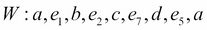 in the City graph is a path.
Also, a graph is known as cyclic if there are one or more paths that start and end at the same node. Such paths are known as cycles. Similarly, if there are no cycles in a graph, it is known as an acyclic graph.
In most of the real-life cases when we would be representing or modeling some event, we would be dealing with a lot of random variables. Even if we would consider all the random variables to be discrete, there would still be exponentially large number of values in the joint probability distribution. Dealing with such huge amount of data would be computationally expensive (and in some cases, even intractable), and would also require huge amount of memory to store the probability of each combination of states of these random variables.
However, in most of the cases, many of these variables are marginally or conditionally independent of each other. By exploiting these independencies, we can reduce the number of values we need to store to represent the joint probability distribution.
For instance, in the previous restaurant example, the joint probability distribution across the four random variables that we discussed (that is, quality of food Q, location of restaurant L, cost of food C, and the number of people visiting N) would require us to store 23 independent values. By the chain rule of probability, we know the following:
P(Q, L, C, N) = P(Q) P(L|Q) P(C|L, Q) P(N|C, Q, L)
Now, let us try to exploit the marginal and conditional independence between the variables, to make the representation more compact. Let's start by considering the independency between the location of the restaurant and quality of food over there. As both of these attributes are independent of each other, P(L|Q) would be the same as P(L). Therefore, we need to store only one parameter to represent it. From the conditional independence that we have seen earlier, we know that  . Thus, P(N|C, Q, L) would be the same as P(N|C, L); thus needing only four parameters. Therefore, we now need only (2 + 1 + 6 + 4 = 13) parameters to represent the whole distribution.
We can conclude that exploiting independencies helps in the compact representation of joint probability distribution. This forms the basis for the Bayesian network.
A Bayesian network is represented by a Directed Acyclic Graph (DAG) and a set of Conditional Probability Distributions (CPD) in which:
In our previous restaurant example, the nodes would be as follows:
Quality of food (Q)
Location (L)
Cost of food (C)
Number of people (N)
As the cost of food was dependent on the quality of food (Q) and the location of the restaurant (L), there will be an edge each from Q → C and L → C. Similarly, as the number of people visiting the restaurant depends on the price of food and its location, there would be an edge each from L → N and C → N. The resulting structure of our Bayesian network is shown in Fig 1.3:
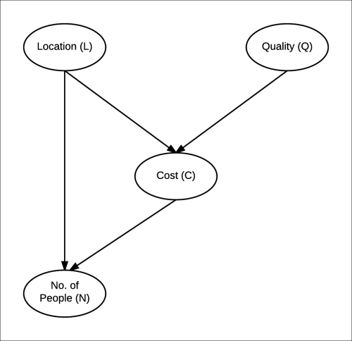
Fig 1.3: Bayesian network for the restaurant example
Each node in our Bayesian network for restaurants has a CPD associated to it. For example, the CPD for the cost of food in the restaurant is P(C|Q, L), as it only depends on the quality of food and location. For the number of people, it would be P(N|C, L) . So, we can generalize that the CPD associated with each node would be P(node|Par(node)) where Par(node) denotes the parents of the node in the graph. Assuming some probability values, we will finally get a network as shown in Fig 1.4:
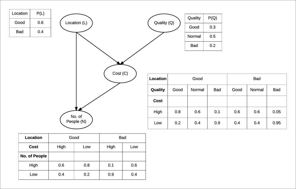
Fig 1.4: Bayesian network of restaurant along with CPDs
Let us go back to the joint probability distribution of all these attributes of the restaurant again. Considering the independencies among variables, we concluded as follows:
P(Q,C,L,N) = P(Q)P(L)P(C|Q, L)P(N|C, L)
So now, looking into the Bayesian network (BN) for the restaurant, we can say that for any Bayesian network, the joint probability distribution  over all its random variables can be represented as follows:
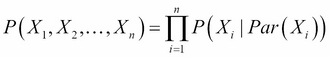
This is known as the chain rule for Bayesian networks.
Also, we say that a distribution P factorizes over a graph G, if P can be encoded as follows:
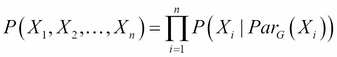
Here,  is the parent of X in the graph G.
Let us consider a more complex Bayesian network of a student getting late for school, as shown in Fig 1.5:
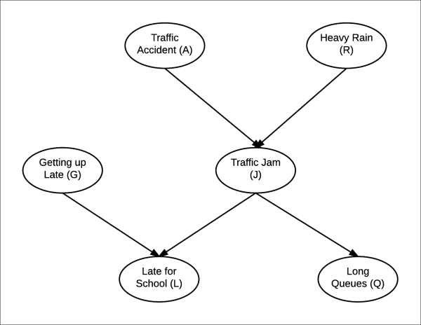
Fig 1.5: Bayesian network representing a particular day of a student going to school
For this Bayesian network, just for simplicity, let us assume that each random variable is discrete with only two possible states {yes, no}.
In pgmpy, we can initialize an empty BN or a model with nodes and edges. We can initializing an empty model as follows:
In [1]: from pgmpy.models import BayesianModel
In [2]: model = BayesianModel()
We can now add nodes and edges to this network:
In [3]: model.add_nodes_from(['rain', 'traffic_jam'])
In [4]: model.add_edge('rain', 'traffic_jam')
If we add an edge, but the nodes, between which the edge is, are not present in the model, pgmpy automatically adds those nodes to the model.
In [5]: model.add_edge('accident', 'traffic_jam')
In [6]: model.nodes()
Out[6]: ['accident', 'rain', 'traffic_jam']
In [7]: model.edges()
Out[7]: [('rain', 'traffic_jam'), ('accident', 'traffic_jam')]
In the case of a Bayesian network, each of the nodes has an associated CPD with it. So, let's define some tabular CPDs to associate with the model:
Note
The name of the variable in tabular CPD should be exactly the same as the name of the node used while creating the Bayesian network, as pgmpy internally uses this name to match the tabular CPDs with the nodes.
In [8]: from pgmpy.factors import TabularCPD
In [9]: cpd_rain = TabularCPD('rain', 2, [[0.4], [0.6]])
In [10]: cpd_accident = TabularCPD('accident', 2, [[0.2], [0.8]])
In [11]: cpd_traffic_jam = TabularCPD(
                                'traffic_jam', 2,
                                [[0.9, 0.6, 0.7, 0.1],
                                 [0.1, 0.4, 0.3, 0.9]],
                                evidence=['rain', 'accident'],
                                evidence_card=[2, 2])
Here, we defined three CPDs. We now need to associate them with our model. To associate them with the model, we just need to use the add_cpd method and pgmpy automatically figures out which CPD is for which node:
In [12]: model.add_cpds(cpd_rain, cpd_accident, cpd_traffic_jam)
In [13]: model.get_cpds()
Out[13]:
[<TabularCPD representing P(rain:2) at 0x7f477b6f9940>,
 <TabularCPD representing P(accident:2) at 0x7f477b6f97f0>,
 <TabularCPD representing P(traffic_jam:2 | rain:2, accident:2) at
                                                  0x7f477b6f9e48>]
Now, let's add the remaining variables and their CPDs:
In [14]: model.add_node('long_queues')
In [15]: model.add_edge('traffic_jam', 'long_queues')
In [16]: cpd_long_queues = TabularCPD('long_queues', 2,
                                      [[0.9, 0.2],
                                       [0.1, 0.8]],
                                      evidence=['traffic_jam'],
                                      evidence_card=[2])
In [17]: model.add_cpds(cpd_long_queues)
In [18]: model.add_nodes_from(['getting_up_late',
                               'late_for_school'])
In [19]: model.add_edges_from(
                   [('getting_up_late', 'late_for_school'),
                    ('traffic_jam', 'late_for_school')])
In [20]: cpd_getting_up_late = TabularCPD('getting_up_late', 2,
                                          [[0.6], [0.4]])
In [21]: cpd_late_for_school = TabularCPD(
                               'late_for_school', 2,
                               [[0.9, 0.45, 0.8, 0.1],
                                [0.1, 0.55, 0.2, 0.9]],
                               evidence=['getting_up_late',
                                         'traffic_jam'],
                               evidence_card=[2, 2])
In [22]: model.add_cpds(cpd_getting_up_late, cpd_late_for_school)
In [23]: model.get_cpds()
Out[23]:
[<TabularCPD representing P(rain:2) at 0x7f477b6f9940>,
 <TabularCPD representing P(accident:2) at 0x7f477b6f97f0>,
 <TabularCPD representing P(traffic_jam:2 | rain:2, accident:2) at
                                                  0x7f477b6f9e48>,
 <TabularCPD representing P(long_queues:2 | traffic_jam:2) at
                                                  0x7f477b7051d0>,
 <TabularCPD representing P(getting_up_late:2) at 0x7f477b7059e8>,
 <TabularCPD representing P(late_for_school:2 | getting_up_late:2,
                                traffic_jam:2) at 0x7f477b705dd8>]
Additionally, pgmpy also provides a check_model method that checks whether the model and all the associated CPDs are consistent:
In [24]: model.check_model()
Out[25]: True
In case we have got some wrong CPD associated with the model and we want to remove it, we can use the remove_cpd method. Let's say we want to remove the CPD associated with variable late_for_school, we could simply do as follows:
In [26]: model.remove_cpds('late_for_school')
In [27]: model.get_cpds()
Out[27]:
[<TabularCPD representing P(rain:2) at 0x7f477b6f9940>,
 <TabularCPD representing P(accident:2) at 0x7f477b6f97f0>,
 <TabularCPD representing P(traffic_jam:2 | rain:2, accident:2) at
                                                  0x7f477b6f9e48>,
 <TabularCPD representing P(long_queues:2 | traffic_jam:2) at
                                                  0x7f477b7051d0>,
<TabularCPD representing P(getting_up_late:2) at 0x7f477b7059e8>]Would the probability of having a road accident change if I knew that there was a traffic jam? Or, what are the chances that it rained heavily today if some student comes late to class? Bayesian networks helps in finding answers to all these questions. Reasoning patterns are key elements of Bayesian networks.
Before answering all these questions, we need to compute the joint probability distribution. For ease in naming the nodes, let's denote them as follows:
Traffic accident as A
Heavy rain as B
Traffic jam as J
Getting up late as G
Long queues as Q
Late to school as L
From the chain rule of the Bayesian network, we have the joint probability distribution  as follows:

Starting with a simple query, what are the chances of having a traffic jam if I know that there was a road accident? This question can be put formally as what is the value of P(J|A = True)?
First, let's compute the probability of having a traffic jam P(J). P(J) can be computed by summing all the cases in the joint probability distribution, where J = True and J = False, and then renormalize the distribution to sum it to 1. We get P(J = True) = 0.416 and P(J = True) = 0.584.
To compute P(J|A = True), we have to eliminate all the cases where A = False, and then we can follow the earlier procedure to get P(J|A = True). This results in P(J = True|A = True) = 0.72 and P(J = False|A = True) = 0.28. We can see that the chances of having a traffic jam increased when we knew that there was an accident. These results match with our intuition. From this, we conclude that the observation of the outcome of the parent in a Bayesian network influences the probability of its children. This is known as causal reasoning. Causal reasoning need not only be the effect of parent on its children; it can go further downstream in the network.
We have seen that the observation of the outcome of parents influence the probability of the children. Is the inverse possible? Let's try to find the probability of heavy rain if we know that there is a traffic accident. To do so, we have to eliminate all the cases where J = False and then reduce the probability to get P(R|J = True). This results in P(R = True|J = True) = 0.7115 and P(R = False|J = True) = 0.2885. This is also intuitive. If we knew that there was a traffic jam, then the chances of heavy rain would increase. This is known as evidential reasoning, where the observation of the outcomes of the children or effect influences the probability of parents or causes.
Let's look at another type of reasoning pattern. If we knew that there was a traffic jam on a day when there was no heavy rain, would it affect the chances of a traffic accident? To do so, we have to follow a similar procedure of eliminating all those cases, except the ones where R = False and J = True. By doing so, we would get P(A = True|J = True, R = False) = 0.6 and P(A = False|J = True, R = False) = 0.4. Now, the probability of an accident increases, which is what we had expected. As we can see that before the observation of the traffic jam, both the random variables, heavy rain and traffic accident, were independent of each other, but with the observation of their common children, they are now dependent on each other. This type of reasoning is called as intercausal reasoning, where different causes with the same effect influence each other.
In the last section, we saw how influence flows in a Bayesian network, and how observing some event changes our belief about other variables in the network. In this section, we will discuss the independence conditions that hold in a Bayesian network no matter which probability distribution is parameterizing the network.
In any network, there can be two types of connections between variables, direct or indirect. Let's start by discussing the direct connection between variables.
In the case of direct connections, we have a direct connection between two variables, that is, there's an edge X → Y in the graph G. In the case of a direct connection, we can always find some probability distribution where they are dependent. Hence, there is no independence condition in a direct connection, no matter which other variables are observed in the network.
In the case of indirect connections, we have four different ways in which the variables can be connected. They are as follows:
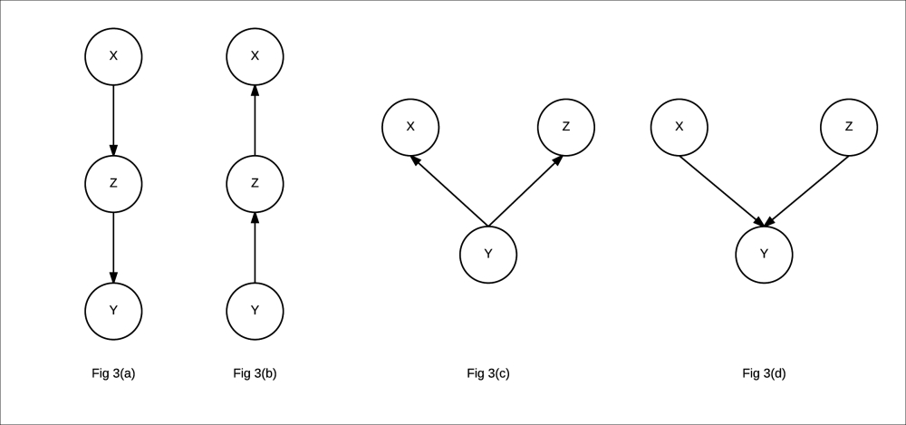
Fig 3(a): Indirect causal relationship
Fig 3(b): Indirect evidential relationship
Fig 3(c): Common cause relationship
Fig 3(d): Common effect relationship
- Indirect causal effect: Fig 3(a) shows an indirect causal relationship between variables X and Y. For intuition, let's consider the late-for-school model, where A → J →L is a causal relationship. Let's first consider the case where J is not observed. If we observe that there has been an accident, then it increases our belief that there would be a traffic jam, which eventually leads to an increase in the probability of getting late for school. Here we see that if the variable J is not observed, then A is able to influence L through J. However, if we consider the case where J is observed, say we have observed that there is a traffic jam, then irrespective of whether there has been an accident or not, it won't change our belief of getting late for school. Therefore, in this case we see that
 .
More often, in the case of an indirect causal relationship
.
More often, in the case of an indirect causal relationship  .
.
- Indirect evidential effect: Fig 3(b) represents an indirect evidential relationship. In the late-for-school model, we can again take the example of L → J ← A. Let's first take the case where we haven't observed J. Now, if we observe that somebody is late for school, it increases our belief that there might be a traffic jam, which increases our belief about there being an accident. This leads us to the same results as we got in the case of an indirect causal effect. The variables X and Y are dependent, but become independent if we observe Z, that is .
Common cause: Fig 3(c) represents a common cause relationship. Let's take the example of L ← J → Q from our late-for-school model. Taking the case where J is not observed, we see that getting late for school makes our belief of being in a traffic jam stronger, which also leads to an increase in the probability of being in a long queue. However, what if we already have observed that there was a traffic jam? In this case, getting late for school doesn't have any effect on being in a long queue. Hence, we see that the independence conditions in this case are also the same as we saw in the previous two cases, that is, X is able to influence Y through Z only if Z is not observed.
Common effect: Fig 3(d) represents a common effect relationship. Taking the example of A → J ← B from the late-for-school model, if we have an observation that there was an accident, it increases the probability of having a traffic jam, but does not have any effect on the probability of heavy rain. Hence, A | B. We see that we have a different observation here than the previous three cases. Now, if we consider the case when J is observed, let's say that there has been a jam. If we now observe that there hasn't been an accident, it does increase the probability that there might have been heavy rain. Hence, A is not independent of B if J is observed. More generally, we can say that in the case of common effect, X is independent of Y if, and only if, Z is not observed.
Now, in a network, how do we know if a variable influences another variable? Let's say we want to check the independence conditions for and  . Also, let's say they are connected by a trail
 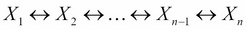 and let Z be the set of observed variables in the Bayesian network. In this case, will be able to influence if and only if the following two conditions are satisfied:
-
For every V structure of the form
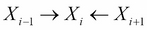 in the trail, either
  or any descendant of
  is an element of Z
 No other node on the trail is in Z
Also, if an influence can flow in a trail in a network, it is known as an active trail. Let's see some examples to check the active trails using pgmpy for the late-for-school model:
In [28]: model.is_active_trail('accident', 'rain')
Out[28]: False
In [29]: model.is_active_trail('accident', 'rain',
                               observed='traffic_jam')
Out[29]: True
In [30]: model.is_active_trail('getting_up_late', 'rain')
Out[30]: False
In [31]: model.is_active_trail('getting_up_late', 'rain',
                               observed='late_for_school')
Out[31]: TrueIn the restaurant example or the late-for-school example, we used the Bayesian network to represent the independencies in the random variables. We also saw that we can use the Bayesian network to represent the joint probability distribution over all the variables using the chain rule. In this section, we will unify these two concepts and show that a probability distribution D can only be represented using a graph G, if and only if D can be represented as a set of CPDs associated with the graph G.
A graph object G is called an IMAP of a probability distribution D if the set of independency assertions in G, denoted by I(G), is a subset of the set of independencies in D, denoted by I(D).
Let's take an example of two random variables X and Y with the following two different probability distributions over it:
|
X |
Y |
P(X, Y) |
|---|---|---|
|
|
|
0.25 |
|
|
|
0.25 |
|
|
|
0.25 |
|
|
|
0.25 |


In this distribution, we can see that P(X) = 0.5 and P(Y) = 0.5. Also, P(X, Y) = P(X)P(Y). Hence, the two random variables X and Y are independent. If we try to represent any two random variables using a network, we have three possibilities:
A graph with two disconnected nodes X and Y
A graph with an edge from X → Y
A graph with an edge from Y → X
We can see from the previous distribution that 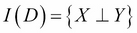 . In the case of disconnected nodes, we also have
 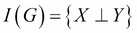 , whereas for the other two graphs, we have I(G) =
 . Hence, all the three graphs are IMAPS of the distribution, and any of these can be used to represent the probability distribution. However, the graph with both nodes disconnected is able to best represent the probability distribution and is known as the Perfect Map.
The structure of the Bayesian network encodes the independencies between the random variables, and every probability distribution for which this BN is an IMAP needs to satisfy these independencies. This allows us to represent the joint probability distribution in a very compact form.
Taking the example of the late-for-school model, using the chain rule, we can show that for any distribution, the joint probability distribution would be as follows:
P(A, R, J, L, S, Q) = P(A) × P(R|A) × P(J|A, R) × P(L|A, R, J) × P(S|A, R, J, L) ×
P(Q|A, R, J, L, S)
However, if we consider a distribution for which the BN is an IMAP, we get information about the independencies in the distribution. As we can see in this example, we know from the Bayesian network structure that S is independent of A and R, given J and L; Q is independent of A, R, and L, and S, given J; and so on. Applying all these conditions on the equation for joint probability distribution reduces it to the following:
P(A, R, J, L, S, Q) = P(A) × P(R) × P(J|A, R) × P(L) × P(S|J, L) × P(Q|J)
Every graph object has associated independencies with it. These independencies allow us to represent the joint probability distribution of the BN in a compact form.
Till now, we have only been working with tabular CPDs. In a tabular CPD, we take all the possible combinations of different states of a variable and represent them in a tabular form. However, in many cases, tabular CPD is not the best choice to represent CPDs. We can take the example of a continuous random variable. As a continuous variable doesn't have states (or let's say infinite states), we can never create a tabular representation for it. There are many other cases which we will discuss in this section when other types of representation are a better choice.
One of the cases when the tabular CPD isn't a good choice is when we have a deterministic random variable, whose value depends only on the values of its parents in the model. For such a variable X with parents Par(X), we have the following:
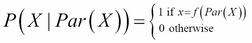
Here, 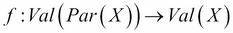 .
.
We can take the example of logic gates (AND, OR, and so on), where the output of the gate is deterministic in nature and depends only on its inputs. We represent it as a Bayesian network, as shown in Fig 1.7:
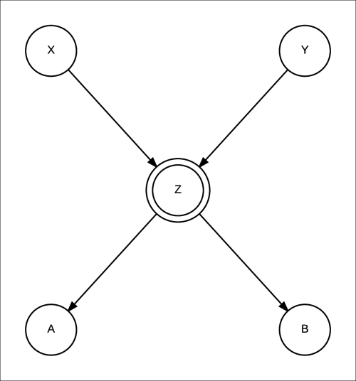
Fig 1.7: A Bayesian network for a logic gate. X and Y are the inputs, A and B are the outputs and Z is a deterministic variable representing the operation of the logic gate.
Here, X and Y are the inputs to the logic gate and Z is the output. We usually denote a deterministic variable by double circles. We can also see that having a deterministic variable gives up more information about the independencies in the network. If we are given the values of X and Y, we know the value of Z, which leads us to the assertion  .
.
We saw the case of deterministic variables where there was a structure in the CPD, which can help us reduce the size of the whole CPD table. As in the case of deterministic variables, structure may occur in many other problems as well. Think of adding a variable Flat Tyre to our late-for-school model. If we have a Flat Tyre (F), irrespective of the values of all other variables, the value of the Late for school variable is always going to be 1. If we think of representing this situation using a tabular CPD, we will have all the values for Late for school corresponding to F = 1 that will be 1, which would essentially be half the table. Hence, if we use tabular CPD, we will be wasting a lot of memory to store values that can simply be represented by a single condition. In such cases, we can use the Tree CPD or Rule CPD.
A great option to represent such context-specific cases is to use a tree structure to represent the various contexts. In a Tree CPD, each leaf represents the various possible conditional distributions, and the path to the leaf represents the conditions for that distribution. Let's take an example by adding a Flat Tyre variable to our earlier model, as shown in Fig 1.8:
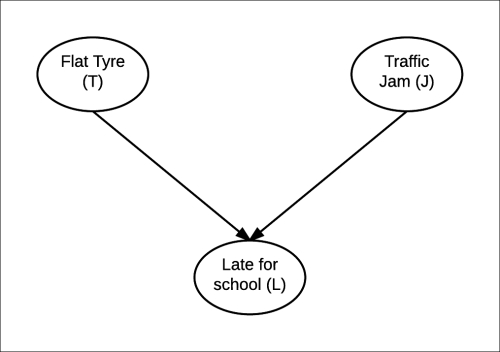
Fig 1.8: Network after adding Flat Tyre (T) variable
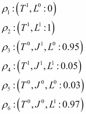
If we represent the CPD of L using a Tree CPD, we will get something like this:
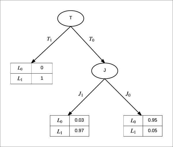
Fig 1.9: Tree CPD in case of Flat tyre
Here, we can see that rather than having four values for the CPD, which we would have to store in the case of Tabular CPD, we only need to store three values in the case of the Tree CPD. This improvement doesn't seem very significant right now, but when we have a large number of variables with high cardinalities, there is a very significant improvement.
Now, let's see how we can implement this using pmgpy:
In [1]: from pgmpy.factors import TreeCPD, Factor
In [2]: tree_cpd = TreeCPD([
                   ('B', Factor(['A'], [2], [0.8, 0.2]), '0'),
                   ('B', 'C', '1'),
                   ('C', Factor(['A'], [2], [0.1, 0.9]), '0'),
                   ('C', 'D', '1'),
                   ('D', Factor(['A'], [2], [0.9, 0.1]), '0'),
('D', Factor(['A'], [2], [0.4, 0.6]), '1')])Rule CPD is another more explicit form of representation of CPDs. Rule CPD is basically a set of rules along with the corresponding values of the variable. Taking the same example of Flat Tyre, we get the following Rule CPD:
Let's see the code implementation using pgmpy:
In [1]: from pgmpy.factors import RuleCPD
In [2]: rule = RuleCPD('A', {('A_0', 'B_0'): 0.8,
                             ('A_1', 'B_0'): 0.2,
                             ('A_0', 'B_1', 'C_0'): 0.4,
                             ('A_1', 'B_1', 'C_0'): 0.6,
                             ('A_0', 'B_1', 'C_1'): 0.9,
('A_1', 'B_1', 'C_1'): 0.1})In this chapter, we saw how we can represent a complex joint probability distribution using a directed graph and a conditional probability distribution associated with each node, which is collectively known as a Bayesian network. We discussed the various reasoning patterns, namely causal, evidential, and intercausal, in a Bayesian network and how changing the CPD of a variable affects other variables. We also discussed the concept of IMAPS, which helped us understand when a joint probability distribution can be encoded in a graph structure.
In the next chapter, we will see that when the relationship between the variables are not causal, a Bayesian model is not sufficient to model our problems. To work with such problems, we will introduce another type of undirected model, known as a Markov model.