The world is consumed with the machine learning revolution and, in particular, the search for a functional artificial general intelligence or AGI. Not to be confused with a conscious AI, AGI is a broader definition of machine intelligence that seeks to apply generalized methods of learning and knowledge to a broad range of tasks, much like the ability we have with our brains—or even small rodents have, for that matter. Rewards-based learning and, in particular, reinforcement learning (RL) are seen as the next steps to a more generalized intelligence.

In this book, we start from the beginning of rewards-based learning and RL with its history to modern inception and its use in gaming and simulation. RL and, specifically, deep RL are gaining popularity in both research and use. In just a few years, the advances in RL have been dramatic, which have made it both impressive but, at the same time, difficult to keep up with and make sense of. With this book, we will unravel the abstract terminology that plagues this multi-branch and complicated topic in detail. By the end of this book, you should be able to consider yourself a confident practitioner of RL and deep RL.

For this first chapter, we will start with an overview of RL and look at the terminology, history, and basic concepts. In this chapter, the high-level topics we will cover are as follows:

• Understanding rewards-based learning
• Introducing the Markov decision process
• Using value learning with multi-armed bandits
• Exploring Q-learning with contextual bandits

We want to mention some important technical requirements before continuing in the next section.

This book is a hands-on one, which means there are plenty of code examples to work through and discover on your own. The code for this book can be found in the following GitHub repository: https://github.com/PacktPublishing/Hands-On-Reinforcement-Learning-for-Games.

As such, be sure to have a working Python coding environment set up. Anaconda, which is a cross-platform wrapper framework for both Python and R, is the recommended platform to use for this book. We also recommend Visual Studio Code or Visual Studio Professional with the Python tools as good Integrated development editors, or IDEs.

With that out of the way, we can move on to learning the basics of RL and, in the next section, look at why rewards-based learning works.

Machine learning is quickly becoming a broad and growing category, with many forms of learning systems addressed. We categorize learning based on the form of a problem and how we need to prepare it for a machine to process. In the case of supervised machine learning, data is first labeled before it is fed into the machine. Examples of this type of learning are simple image classification systems that are trained to recognize a cat or dog from a prelabeled set of cat and dog images. Supervised learning is the most popular and intuitive type of learning system. Other forms of learning that are becoming increasingly powerful are unsupervised and semi-supervised learning. Both of these methods eliminate the need for labels or, in the case of semi-supervised learning, require the labels to be defined more abstractly. The following diagram shows these learning methods and how they process data:

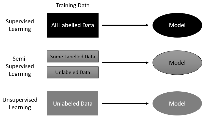
While this family of supervised learning methods has made impressive progress in just the last few years, they still lack the necessary planning and intelligence we expect from a truly intelligent machine. This is where RL picks up and differentiates itself. RL systems learn from interacting and making selections in the environment the agent resides in. The classic diagram of an RL system is shown here:

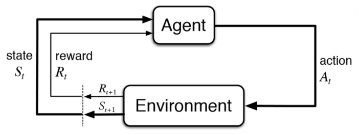
An RL system

In the preceding diagram, you can identify the main components of an RL system: the Agent and Environment, where the Agent represents the RL system, and the Environment could be representative of a game board, game screen, and/or possibly streaming data. Connecting these components are three primary signals, the State, Reward, and Action. The State signal is essentially a snapshot of the current state of Environment. The Reward signal may be externally provided by the Environment and provides feedback to the agent, either bad or good. Finally, the Action signal is the action the Agent selects at each time step in the environment. An action could be as simple as jump or a more complex set of controls operating servos. Either way, another key difference in RL is the ability for the agent to interact with, and change, the Environment.

Now, don't worry if this all seems a little muddled still—early researchers often encountered trouble differentiating between supervised learning and RL.

In the next section, we look at more RL terminology and explore the basic elements of an RL agent.

Every RL agent is comprised of four main elements. These are policy, reward function, value function, and, optionally, model. Let's now explore what each of these terms means in more detail:

• The policy: A policy represents the decision and planning process of the agent. The policy is what decides the actions the agent will take during a step.
• The reward function: The reward function determines what amount of reward an agent receives after completing a series of actions or an action. Generally, a reward is given to an agent externally but, as we will see, there are internal reward systems as well.
• The value function: A value function determines the value of a state over the long term. Determining the value of a state is fundamental to RL and our first exercise will be determining state values.
• The model: A model represents the environment in full. In the case of a game of tic-tac-toe, this may represent all possible game states. For more advanced RL algorithms, we use the concept of a partially observable state that allows us to do away with a full model of the environment. Some environments that we will tackle in this book have more states than the number of atoms in the universe. Yes, you read that right. In massive environments like that, we could never hope to model the entire environment state.

We will spend the next several chapters covering each of these terms in excruciating detail, so don't worry if things feel a bit abstract still. In the next section, we will take a look at the history of RL.

An Introduction to RL, by Sutton and Barto (1998), discusses the origins of modern RL being derived from two main threads with a later joining thread. The two main threads are trial and error-based learning and dynamic programming, with the third thread arriving later in the form of temporal difference learning. The primary thread founded by Sutton, trial and error, is based on animal psychology. As for the other methods, we will look at each in far more detail in their respective chapters. A diagram showing how these three threads converged to form modern RL is shown here:

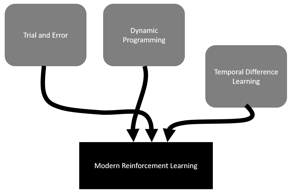
The history of modern RL

Lastly, before we jump in and start unraveling RL, let's look at why it makes sense to use this form of learning with games in the next section.

Various forms of machine learning systems have been used in gaming, with supervised learning being the primary choice. While these methods can be made to look intelligent, they are still limited by working on labeled or categorized data. While generative adversarial networks (GANs) show a particular promise in level and other asset generation, these families of algorithms cannot plan and make sense of long-term decision making. AI systems that replicate planning and interactive behavior in games are now typically done with hardcoded state machine systems such as finite state machines or behavior trees. Being able to develop agents that can learn for themselves the best moves or actions for an environment is literally game-changing, not only for the games industry, of course, but this should surely cause repercussions in every industry globally.

In the next section, we take a look at the foundation of the RL system, the Markov decision process.

In RL, the agent learns from the environment by interpreting the state signal. The state signal from the environment needs to define a discrete slice of the environment at that time. For example, if our agent was controlling a rocket, each state signal would define an exact position of the rocket in time. State, in that case, may be defined by the rocket's position and velocity. We define this state signal from the environment as a Markov state. The Markov state is not enough to make decisions from, and the agent needs to understand previous states, possible actions, and any future rewards. All of these additional properties may converge to form a Markov property, which we will discuss further in the next section.

An RL problem fulfills the Markov property if all Markov signals/states predict a future state. Subsequently, a Markov signal or state is considered a Markov property if it enables the agent to predict values from that state. Likewise, a learning task that is a Markov property and is finite is called a finite Markov decision process, or MDP. A very classic example of an MDP used to often explain RL is shown here:

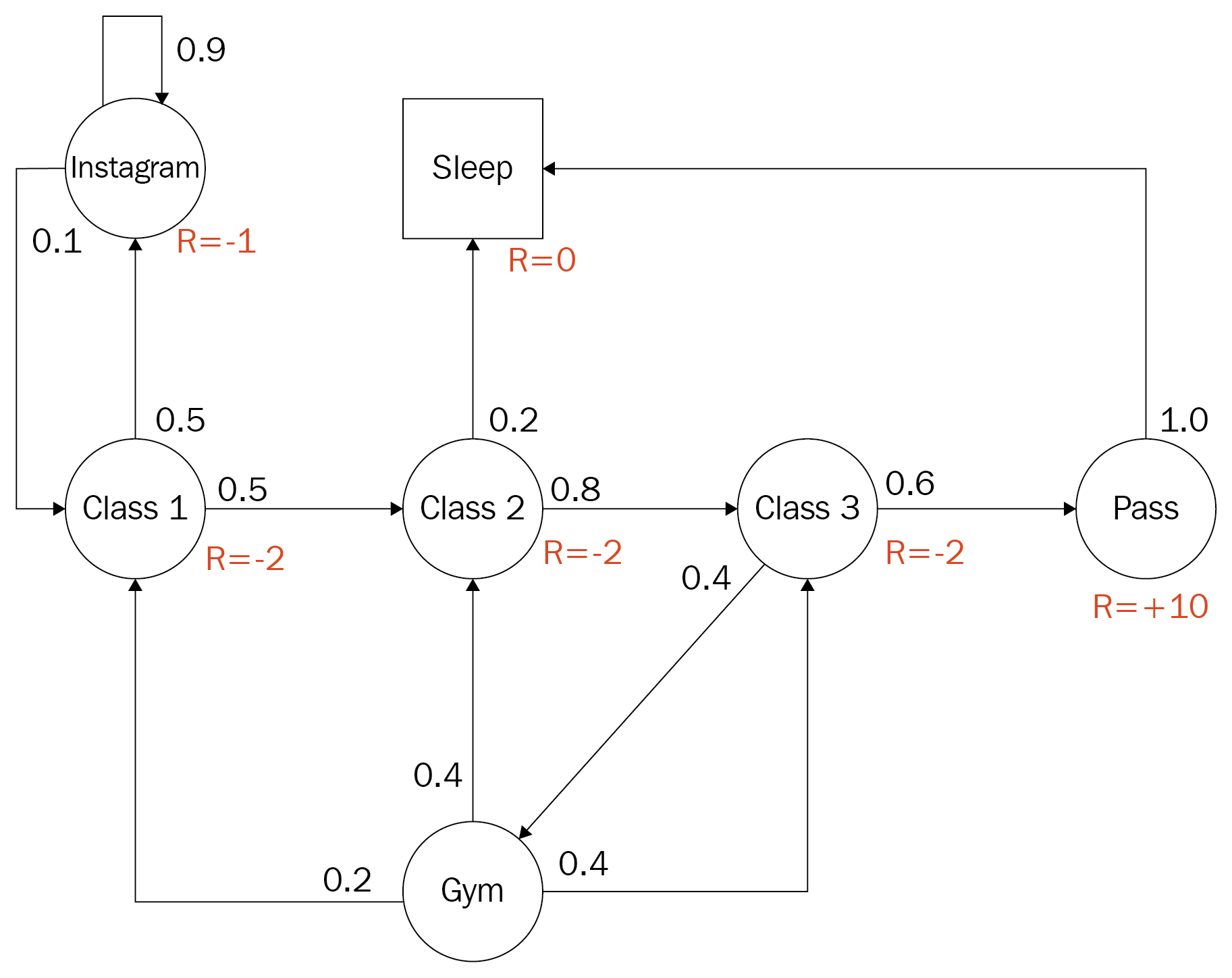
The Markov decision process (Dr. David Silver)

The diagram is an example of a finite discrete MDP for a post-secondary student trying to optimize their actions for maximum reward. The student has the option of attending class, going to the gym, hanging out on Instagram or whatever, passing and/or sleeping. States are denoted by circles and the text defines the activity. In addition to this, the numbers next to each path from a circle denote the probability of using that path. Note how all of the values around a single circle sum to 1.0 or 100% probability. The R= denotes the reward or output of the reward function when the student is in that state. To solidify this abstract concept further, let's build our own MDP in the next section.

In this hands-on exercise, we will build an MDP using a task from your own daily life or experience. This should allow you to better apply this abstract concept to something more tangible. Let's begin as follows:

1. Think of a daily task you do that may encompass six or so states. Examples of this may be going to school, getting dressed, eating, showering, browsing Facebook, and traveling.
2. Write each state within a circle on a full sheet of paper or perhaps some digital drawing app.
3. Connect the states with the actions you feel most appropriate. For example, don't get dressed before you shower.
4. Assign the probability you would use to take each action. For example, if you have two actions leaving a state, you could make them both 50/50 or 0.5/0.5, or some other combination that adds up to 1.0.
5. Assign the reward. Decide what rewards you would receive for being within each state and mark those on your diagram.
6. Compare your completed diagram with the preceding example. How did you do?

Before we get to solving your MDP or others, we first need to understand some background on calculating values. We will uncover this in the next section.

Solving a full MDP and, hence, the full RL problem first requires us to understand values and how we calculate the value of a state with a value function. Recall that the value function was a primary element of the RL system. Instead of using a full MDP to explain this, we instead rely on a simpler single-state problem known as the multi-armed bandit problem. This is named after the one-armed slot machines often referred to as bandits by their patrons but, in this case, the machine has multiple arms. That is, we now consider a single-state or stationary problem with multiple actions that lead to terminal states providing constant rewards. More simply, our agent is going to play a multi-arm slot machine that will give either a win or loss based on the arm pulled, with each arm always returning the same reward. An example of our agent playing this machine is shown here:

We can consider the value for a single state to be dependent on the next action, provided we also understand the reward provided by that action. Mathematically, we can define a simple value equation for learning like so:

In this equation, we have the following:

• V(a): the value for a given action
• a: action
• α: alpha or the learning rate
• r: reward

Notice the addition of a new variable called α (alpha) or the learning rate. This learning rate denotes how fast the agent needs to learn the value from pull to pull. The smaller the learning rate (0.1), the slower the agent learns. This method of action-value learning is fundamental to RL. Let's code up this simple example to solidify further in the next section.

Since this is our first example, make sure your Python environment is set to go. Again for simplicity, we prefer Anaconda. Make sure you are comfortable coding with your chosen IDE and open up the code example, Chapter_1_1.py, and follow along:

1. Let's examine the first section of the code, as shown here:

import random

reward = [1.0, 0.5, 0.2, 0.5, 0.6, 0.1, -.5]
arms = len(reward)
episodes = 100
learning_rate = .1
Value = [0.0] * arms
print(Value)

2. We first start by doing import of random. We will use random to randomly select an arm during each training episode.
3. Next, we define a list of rewards, reward. This list defines the reward for each arm (action) and hence defines the number of arms/actions on the bandit.
4. Then, we determine the number of arms using the len() function.
5. After that, we set the number of training episodes our agent will use to evaluate the value of each arm.
6. Set the learning_rate value to .1. This means the agent will learn slowly the value of each pull.
7. Next, we initialize the value for each action in a list called Value, using the following code:

Value = [0.0] * arms

8. Then, we print the Value list to the console, making sure all of the values are 0.0.

The first section of code initialized our rewards, number of arms, learning rate, and value list. Now, we need to implement the training cycle where our agent/algorithm will learn the value of each pull. Let's jump back into the code for Chapter_1_1.py and look to the next section:

1. The next section of code in the listing we want to focus on is entitled agent learns and is shown here for reference:

# agent learns
for i in range(0, episodes):
    action = random.randint(0,arms-1)
    Value[action] = Value[action] + learning_rate * (
        reward[action] - Value[action])

print(Value)

2. We start by first defining a for loop that loops through 0 to our number of episodes. For each episode, we let the agent pull an arm and use the reward from that pull to update its determination of value for that action or arm.
3. Next, we want to determine the action or arm the agent pulls randomly using the following code:

action = random.randint(0,arms-1)

4. The code just selects a random arm/action number based on the total number of arms on the bandit (minus one to allow for proper indexing).
5. This then allows us to determine the value of the pull by using the next line of code, which mirrors very well our previous value equation:

Value[action] = Value[action] + learning_rate * (       reward[action] - Value[action])

6. That line of code clearly resembles the math for our previous Value equation. Now, think about how learning_rate is getting applied during each iteration of an episode. Notice that, with a rate of .1, our agent is learning or applying 1/10^th of what reward the agent receives minus the Value function the agent previously equated. This little trick has the effect of averaging out the values across the episodes.
7. Finally, after the looping completes and all of the episodes are run, we print the updated Value function for each action.
8. Run the code from the command line or your favorite Python editor. In Visual Studio, this is as simple as hitting the play button. After the code has completed running, you should see something similar to the following, but not the exact output:

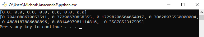
Now, think back and compare those output values to the rewards set for each arm. Are they the same or different and if so, by how much? Generally, the learned values after only 100 episodes should indicate a clear value but likely not the finite value. This means the values will be smaller than the final rewards but they should still indicate a preference.

The solution we show here is an example of trial and error learning; it's that first thread we talked about back in the history of RL section. As you can see, the agent learns by randomly pulling an arm and determining the value. However, at no time does our agent learn to make better decisions based on those updated values. The agent always just pulls randomly. Our agent currently has no decision mechanism or what we call a policy in RL. We will look at how to implement a basic greedy policy in the next section.

Our current value learner is not really learning aside from finding the optimum calculated value or the reward for each action over several episodes. Since our agent is not learning, it also makes it a less efficient learner as well. After all, the agent is just randomly picking any arm each episode when it could be using its acquired knowledge, which is the Value function, to determine it's next best choice. We can code this up in a very simple policy called a greedy policy in the next exercise:

1. Open up the Chapter_1_2.py example. The code is basically the same as our last example except for the episode iteration and, in particular, the selection of action or arm. The full listing can be seen here—note the new highlighted sections:

import random

reward = [1.0, 0.5, 0.2, 0.5, 0.6, 0.1, -.5]
arms = len(reward)
learning_rate = .1
episodes = 100
Value = [0.0] * arms
print(Value)

def greedy(values):
    return values.index(max(values))

# agent learns
for i in range(0, episodes):
    action = greedy(Value)
    Value[action] = Value[action] + learning_rate * (
        reward[action] - Value[action])

print(Value)

2. Notice the inclusion of a new greedy() function. This function will always select the action with the highest value and return the corresponding index/action index. This function is essentially our agent's policy.
3. Scrolling down in the code, notice inside the training loop how we are now using the greedy() function to select our action, as shown here:

action = greedy(Value)

4. Again, run the code and look at the output. Is it what you expected? What went wrong?

Looking at your output likely shows that the agent calculated the maximum reward arm correctly, but likely didn't determine the correct values for the other arms. The reason for this is that, as soon as the agent found the most valuable arm, it kept pulling that arm. Essentially the agent finds the best path and sticks with it, which is okay in this single step or stationary environment but certainly won't work over a many step problem requiring multiple decisions. Instead, we need to balance the agents need to explore and find new paths, versus maximizing the immediate optimum reward. This problem is called the exploration versus exploitation dilemma in RL and something we will explore in the next section.

As we have seen, having our agent always make the best choice limits their ability to learn the full values of a single state never mind multiple connected states. This also severely limits an agent's ability to learn, especially in environments where multiple states converge and diverge. What we need, therefore, is a way for our agent to choose an action based on a policy that favors more equal action/value distribution. Essentially, we need a policy that allows our agent to explore as well as exploit its knowledge to maximize learning. There are multiple variations and ways of balancing the trade-off between exploration and exploitation. Much of this will depend on the particular environment as well as the specific RL implementation you are using. We would never use an absolute greedy policy but, instead, some variation of greedy or another method entirely. In our next exercise, we show how to implement an initial optimistic value method, which can be effective:

1. Open Chapter_1_3.py and look at the highlighted lines shown here:

episodes = 10000
Value = [5.0] * arms

2. First, we have increased the number of episodes to 10000. This will allow us to confirm that our new policy is converging to some appropriate solution.

3. Next, we set the initial value of the Value list to 5.0. Note that this value is well above the reward value maximum of 1.0. Using a higher value than our reward forces our agent to always explore the most valuable path, which now becomes any path it hasn't explored, hence ensuring our agent will always explore each action or arm at least once.
4. There are no more code changes and you can run the example as you normally would. The output of the example is shown here:

Your output may vary slightly but it likely will show very similar values. Notice how the calculated values are now more relative. That is, the value of 1.0 clearly indicates the best course of action, the arm with a reward of 1.0, but the other values are less indicative of the actual reward. Initial option value methods are effective but will force an agent to explore all paths, which are not so efficient in larger environments. There are of course a multitude of other methods you can use to balance exploration versus exploitation and we will cover a new method in the next section, where we introduce solving the full RL problem with Q-learning.

Now that we understand how to calculate values and the delicate balance of exploration and exploitation, we can move on to solving an entire MDP. As we will see, various solutions work better or worse depending on the RL problem and environment. That is actually the basis for the next several chapters. For now, though, we just want to introduce a method that is basic enough to solve the full RL problem. We describe the full RL problem as the non-stationary or contextual multi-armed bandit problem, that is, an agent that moves across a different bandit each episode and chooses a single arm from multiple arms. Each bandit now represents a different state and we no longer want to determine just the value of an action but the quality. We can calculate the quality of an action given a state using the Q-learning equation shown here:

In the preceding equation, we have the following:

• : state
• : current state
• : next action
• : current action
• ϒ: gamma—reward discount
• α: alpha—learning rate
• r: reward
• : next reward
• : quality

Now, don't get overly concerned if all of these terms are a little foreign and this equation appears overwhelming. This is the Q-learning equation developed by Chris Watkins in 1989 and is a method that simplifies the solving of a Finite Markov Decision Process or FMDP. The important thing to observe about the equation at this point is to understand the similarities it shares with the earlier action-value equation. In Chapter 2, Dynamic Programming and the Bellman Equation, we will learn in more detail how this equation is derived and functions. For now, the important concept to grasp is that we are now calculating a quality-based value on previous states and rewards based on actions rather than just a single action-value. This, in turn, allows our agent to make better planning for multiple states. We will implement a Q-learning agent that can play several multi-armed bandits and be able to maximize rewards in the next section.

While that Q-learning equation may seem a lot more complex, actually implementing the equation is not unlike building our agent that just learned values earlier. To keep things simpler, we will use the same base of code but turn it into a Q-learning example. Open up the code example, Chapter_1_4.py, and follow the exercise here:

1. Here is the full code listing for reference:

import random

arms = 7
bandits = 7
learning_rate = .1
gamma = .9
episodes = 10000

reward = []
for i in range(bandits):  
    reward.append([])       
    for j in range(arms): 
        reward[i].append(random.uniform(-1,1))
print(reward)

Q = []
for i in range(bandits):  
    Q.append([])       
    for j in range(arms): 
        Q[i].append(10.0)
print(Q)

def greedy(values):
    return values.index(max(values))

def learn(state, action, reward, next_state):
    q = gamma * max(Q[next_state])
    q += reward
    q -= Q[state][action]
    q *= learning_rate
    q += Q[state][action]
    Q[state][action] = q

# agent learns
bandit = random.randint(0,bandits-1)
for i in range(0, episodes):
    last_bandit = bandit
    bandit = random.randint(0,bandits-1)
    action = greedy(Q[bandit]) 
    r = reward[last_bandit][action]
    learn(last_bandit, action, r, bandit)
print(Q)

2. All of the highlighted sections of code are new and worth paying closer attention to. Let's take a look at each section in more detail here:

arms = 7
bandits = 7
gamma = .9 

3. We start by initializing the arms variable to 7 then a new bandits variable to 7 as well. Recall that arms is analogous to actions and bandits likewise is to state. The last new variable, gamma, is a new learning parameter used to discount rewards. We will explore this discount factor concept in future chapters:

reward = []
for i in range(bandits):
    reward.append([]) 
    for j in range(arms):
        reward[i].append(random.uniform(-1,1))
print(reward)

4. The next section of code builds up the reward table matrix as a set of random values from -1 to 1. We use a list of lists in this example to better represent the separate concepts:

Q = []
for i in range(bandits):  
    Q.append([])     
    for j in range(arms): 
        Q[i].append(10.0)
print(Q)

5. The following section is very similar and this time sets up a Q table matrix to hold our calculated quality values. Notice how we initialize our starting Q value to 10.0. We do this to account for subtle changes in the math, again something we will discuss later.
6. Since our states and actions can be all mapped onto a matrix/table, we refer to our RL system as using a model. A model represents all actions and states of an environment:

def learn(state, action, reward, next_state):
    q = gamma * max(Q[next_state])
    q += reward
    q -= Q[state][action]
    q *= learning_rate
    q += Q[state][action]
    Q[state][action] = q

7. We next define a new function called learn. This new function is just a straight implementation of the Q equation we observed earlier:

bandit = random.randint(0,bandits-1)
for i in range(0, episodes):
    last_bandit = bandit
    bandit = random.randint(0,bandits-1)
    action = greedy(Q[bandit]) 
    r = reward[last_bandit][action]
    learn(last_bandit, action, r, bandit)
print(Q)

8. Finally, the agent learning section is updated significantly with new code. This new code sets up the parameters we need for the new learn function we looked at earlier. Notice how the bandit or state is getting randomly selected each time. Essentially, this means our agent is just randomly walking from bandit to bandit.
9. Run the code as you normally would and notice the new calculated Q values printed out at the end. Do they match the rewards for each of the arm pulls?

Likely, a few of your arms don't match up with their respective reward values. This is because the new Q-learning equation solves the entire MDP but our agent is NOT moving in an MDP. Instead, our agent is just randomly moving from state to state with no care on which state it saw before. Think back to our example and you will realize since our current state does not affect our future state, it fails to be a Markov property and hence is not an MDP. However, that doesn't mean we can't successfully solve this problem and we will look to do that in the next section.

The problem with our current solution and using the full Q-learning equation is that the equation assumes any state our agent is in affects future states. Except, remember in our example, the agent just walked randomly from bandit to bandit. This means using any previous state information would be useless, as we saw. Fortunately, we can easily fix this by removing the concept of discounted rewards. Recall that new variable, gamma, that appeared in this complicated term: . Gamma and this term are a way of discounting future rewards and something we will discuss at length starting in Chapter 2, Dynamic Programming and the Bellman Equation. For now, though, we can fix this sample up by just removing that term from our learn function. Let's open up code example, Chapter_1_5.py, and follow the exercise here:

1. The only section of code we really need to focus on is the updated learn function, here:

def learn(state, action, reward, next_state):
    #q = gamma * max(Q[next_state])
    q = 0
    q += reward
    q -= Q[state][action]
    q *= learning_rate
    q += Q[state][action]
    Q[state][action] = q

2. The first line of code in the function is responsible for discounting the future reward of the next state. Since none of the states in our example are connected, we can just comment out that line. We create a new initializer for q = 0 in the next line.
3. Run the code as you normally would. Now you should see very close values closely matching their respective rewards.

By omitting the discounted rewards part of the calculation, hopefully, you can appreciate that this would just revert to a value calculation problem. Alternatively, you may also realize that if our bandits were connected. That is, pulling an arm led to another one arm machine with more actions and so on. We could then use the Q-learning equation to solve the problem as well.

That concludes a very basic introduction to the primary components and elements of RL. Throughout the rest of this book, we will dig into the nuances of policies, values, actions, and rewards.

In this chapter, we first introduced ourselves to the world of RL. We looked at what makes RL so unique and why it makes sense for games. After that, we explored the basic terminology and history of modern RL. From there, we looked to the foundations of RL and the Markov decision process, where we discovered what makes an RL problem. Then we looked to building our first learner a value learner that calculated the values of states on an action. This led us to uncover the need for exploration and exploitation and the dilemma that constantly challenges RL implementers. Next, we jumped in and discovered the full Q-learning equation and how to build a Q-learner, where we later realized that the full Q equation was beyond what we needed for our unconnected state environment. We then reverted our Q learned back into a value learner and watched it solve the contextual bandit problem.

In the next chapter, we will continue from where we left off and look into how rewards are discounted with the Bellman equation, as well as look at the many other improvements dynamic programming has introduced to RL.

Use these questions and exercises to reinforce the material you just learned. The exercises may be fun to attempt, so be sure to try atleast two to four questions/exercises:

Questions:

1. What are the names of the main components of an RL system? Hint, the first one is Environment.
2. Name the four elements of an RL system. Remember that one element is optional.
3. Name the three main threads that compose modern RL.
4. What makes a Markov state a Markov property?
5. What is a policy?

Exercises:

1. Using Chapter_1_2.py, alter the code so the agent pulls from a bandit with 1,000 arms. What code changes do you need to make?
2. Using Chapter_1_3.py, alter the code so that the agent pulls from the average value, not greedy/max. How did this affect the agent's exploration?
3. Using Chapter_1_3.py, alter the learning_rate variable to determine how fast or slow you can make the agent learn. How few episodes are you required to run for the agent to solve the problem?
4. Using Chapter_1_5.py, alter the code so that the agent uses a different policy (either the greedy policy or something else). Take points off yourself if you look ahead in this book or online for solutions.
5. Using Chapter_1_4.py, alter the code so that the bandits are connected. Hence, when an agent pulls an arm, they receive a reward and are transported to another specific bandit, no longer at random. Hint: This likely will require a new destination table to be built and you will now need to include the discounted reward term we removed.

Even completing a few of these questions and/or exercises will make a huge difference to your learning this material. This is a hands-on book after all.