OpenAI is an artificial intelligence (AI) research organization that aims to build artificial general intelligence (AGI). OpenAI provides a famous toolkit called Gym for training a reinforcement learning agent.

Let's suppose we need to train our agent to drive a car. We need an environment to train the agent. Can we train our agent in the real-world environment to drive a car? No, because we have learned that reinforcement learning (RL) is a trial-and-error learning process, so while we train our agent, it will make a lot of mistakes during learning. For example, let's suppose our agent hits another vehicle, and it receives a negative reward. It will then learn that hitting other vehicles is not a good action and will try not to perform this action again. But we cannot train the RL agent in the real-world environment by hitting other vehicles, right? That is why we use simulators and train the RL agent in the simulated environments.

There are many toolkits that provide a simulated environment for training an RL agent. One such popular toolkit is Gym. Gym provides a variety of environments for training an RL agent ranging from classic control tasks to Atari game environments. We can train our RL agent to learn in these simulated environments using various RL algorithms. In this chapter, first, we will install Gym and then we will explore various Gym environments. We will also get hands-on with the concepts we have learned in the previous chapter by experimenting with the Gym environment.

Throughout the book, we will use the Gym toolkit for building and evaluating reinforcement learning algorithms, so in this chapter, we will make ourselves familiar with the Gym toolkit.

In this chapter, we will learn about the following topics:

• Setting up our machine
• Installing Anaconda and Gym
• Understanding the Gym environment
• Generating an episode in the Gym environment
• Exploring more Gym environments
• Cart-Pole balancing with the random agent
• An agent playing the Tennis game

In this section, we will learn how to install several dependencies that are required for running the code used throughout the book. First, we will learn how to install Anaconda and then we will explore how to install Gym.

Installing Anaconda

Anaconda is an open-source distribution of Python. It is widely used for scientific computing and processing large volumes of data. It provides an excellent package management environment, and it supports Windows, Mac, and Linux operating systems. Anaconda comes with Python installed, along with popular packages used for scientific computing such as NumPy, SciPy, and so on.

To download Anaconda, visit https://www.anaconda.com/download/, where you will see an option for downloading Anaconda for different platforms. If you are using Windows or macOS, you can directly download the graphical installer according to your machine architecture and install Anaconda using the graphical installer.

If you are using Linux, follow these steps:

1. Open the Terminal and type the following command to download Anaconda:

   wget https://repo.continuum.io/archive/Anaconda3-5.0.1-Linux-x86_64.sh
   

2. After downloading, we can install Anaconda using the following command:

   bash Anaconda3-5.0.1-Linux-x86_64.sh
   

After the successful installation of Anaconda, we need to create a virtual environment. What is the need for a virtual environment? Say we are working on project A, which uses NumPy version 1.14, and project B, which uses NumPy version 1.13. So, to work on project B we either downgrade NumPy or reinstall NumPy. In each project, we use different libraries with different versions that are not applicable to the other projects. Instead of downgrading or upgrading versions or reinstalling libraries every time for a new project, we use a virtual environment.

The virtual environment is just an isolated environment for a particular project so that each project can have its own dependencies and will not affect other projects. We will create a virtual environment using the following command and name our environment universe:

conda create --name universe python=3.6 anaconda

Note that we use Python version 3.6. Once the virtual environment is created, we can activate it using the following command:

source activate universe

That's it! Now that we have learned how to install Anaconda and create a virtual environment, in the next section, we will learn how to install Gym.

Installing the Gym toolkit

In this section, we will learn how to install the Gym toolkit. Before going ahead, first, let's activate our virtual environment, universe:

source activate universe

Now, install the following dependencies:

sudo apt-get update
sudo apt-get install golang libcupti-dev libjpeg-turbo8-dev make tmux htop chromium-browser git cmake zlib1g-dev libjpeg-dev xvfb libav-tools xorg-dev python-opengl libboost-all-dev libsdl2-dev swig
conda install pip six libgcc swig
conda install opencv

We can install Gym directly using pip. Note that throughout the book, we will use Gym version 0.15.4. We can install Gym using the following command:

pip install gym==0.15.4

We can also install Gym by cloning the Gym repository as follows:

cd ~
git clone https://github.com/openai/gym.git
cd gym
pip install -e '.[all]'

Common error fixes

Just in case, if you get any of the following errors while installing Gym, the following commands will help:

• Failed building wheel for pachi-py or failed building wheel for pachi-py atari-py:

  sudo apt-get update
  sudo apt-get install xvfb libav-tools xorg-dev libsdl2-dev swig cmake
  

• Failed building wheel for mujoco-py:

  git clone https://github.com/openai/mujoco-py.git
  cd mujoco-py
  sudo apt-get update
  sudo apt-get install libgl1-mesa-dev libgl1-mesa-glx libosmesa6-dev python3-pip python3-numpy python3-scipy
  pip3 install -r requirements.txt
  sudo python3 setup.py install
  

• error: command 'gcc' failed with exit status 1:

  sudo apt-get update
  sudo apt-get install python-dev 
  sudo apt-get install libevent-dev
  

Now that we have successfully installed Gym, in the next section, let's kickstart our hands-on reinforcement learning journey.

We have learned that Gym provides a variety of environments for training a reinforcement learning agent. To clearly understand how the Gym environment is designed, we will start with the basic Gym environment. After that, we will understand other complex Gym environments.

Let's introduce one of the simplest environments called the Frozen Lake environment. Figure 2.1 shows the Frozen Lake environment. As we can observe, in the Frozen Lake environment, the goal of the agent is to start from the initial state S and reach the goal state G:

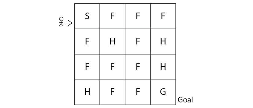
Figure 2.1: The Frozen Lake environment

In the preceding environment, the following apply:

• S denotes the starting state
• F denotes the frozen state
• H denotes the hole state
• G denotes the goal state

So, the agent has to start from state S and reach the goal state G. But one issue is that if the agent visits state H, which is the hole state, then the agent will fall into the hole and die as shown in Figure 2.2:

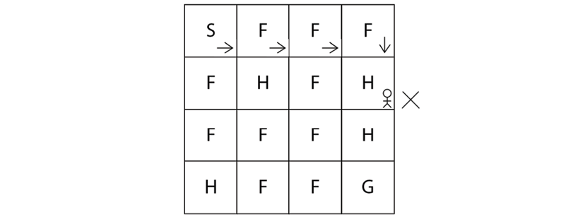
Figure 2.2: The agent falls down a hole

So, we need to make sure that the agent starts from S and reaches G without falling into the hole state H as shown in Figure 2.3:

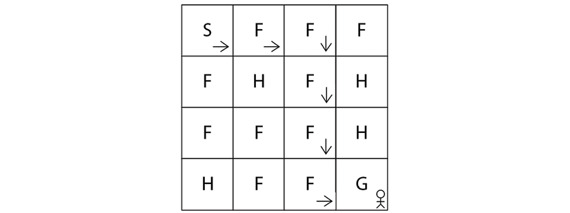
Figure 2.3: The agent reaches the goal state

Each grid box in the preceding environment is called a state, thus we have 16 states (S to G) and we have 4 possible actions, which are up, down, left, and right. We learned that our goal is to reach the state G from S without visiting H. So, we assign +1 reward for the goal state G and 0 for all other states.

Thus, we have learned how the Frozen Lake environment works. Now, to train our agent in the Frozen Lake environment, first, we need to create the environment by coding it from scratch in Python. But luckily we don't have to do that! Since Gym provides various environments, we can directly import the Gym toolkit and create a Frozen Lake environment.

Now, we will learn how to create our Frozen Lake environment using Gym. Before running any code, make sure that you have activated our virtual environment universe. First, let's import the Gym library:

import gym

Next, we can create a Gym environment using the make function. The make function requires the environment id as a parameter. In Gym, the id of the Frozen Lake environment is FrozenLake-v0. So, we can create our Frozen Lake environment as follows:

env = gym.make("FrozenLake-v0")

After creating the environment, we can see how our environment looks like using the render function:

env.render()

The preceding code renders the following environment:

Figure 2.4: Gym's Frozen Lake environment

As we can observe, the Frozen Lake environment consists of 16 states (S to G) as we learned. The state S is highlighted indicating that it is our current state, that is, the agent is in the state S. So whenever we create an environment, an agent will always begin from the initial state, which in our case is state S.

That's it! Creating the environment using Gym is that simple. In the next section, we will understand more about the Gym environment by relating all the concepts we have learned in the previous chapter.

Exploring the environment

In the previous chapter, we learned that the reinforcement learning environment can be modeled as a Markov decision process (MDP) and an MDP consists of the following:

• States: A set of states present in the environment.
• Actions: A set of actions that the agent can perform in each state.
• Transition probability: The transition probability is denoted by . It implies the probability of moving from a state s to the state while performing an action a.
• Reward function: The reward function is denoted by . It implies the reward the agent obtains moving from a state s to the state while performing an action a.

Let's now understand how to obtain all the above information from the Frozen Lake environment we just created using Gym.

States

A state space consists of all of our states. We can obtain the number of states in our environment by just typing env.observation_space as follows:

print(env.observation_space)

The preceding code will print:

Discrete(16)

It implies that we have 16 discrete states in our state space starting from state S to G. Note that, in Gym, the states will be encoded as a number, so the state S will be encoded as 0, state F will be encoded as 1, and so on as Figure 2.5 shows:

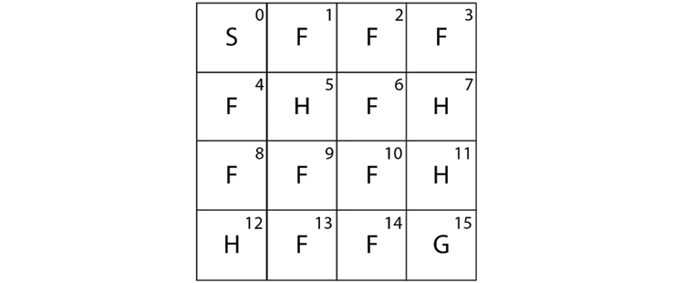
Figure 2.5: Sixteen discrete states

Actions

We learned that the action space consists of all the possible actions in the environment. We can obtain the action space by using env.action_space:

print(env.action_space)

The preceding code will print:

Discrete(4)

It shows that we have 4 discrete actions in our action space, which are left, down, right, and up. Note that, similar to states, actions also will be encoded into numbers as shown in Table 2.1:

Table 2.1: Four discrete actions

Transition probability and reward function

Now, let's look at how to obtain the transition probability and the reward function. We learned that in the stochastic environment, we cannot say that by performing some action a, the agent will always reach the next state exactly because there will be some randomness associated with the stochastic environment, and by performing an action a in the state s, the agent reaches the next state with some probability.

Let's suppose we are in state 2 (F). Now, if we perform action 1 (down) in state 2, we can reach state 6 as shown in Figure 2.6:

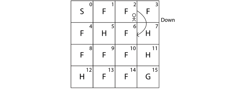
Figure 2.6: The agent performing a down action from state 2

Our Frozen Lake environment is a stochastic environment. When our environment is stochastic, we won't always reach state 6 by performing action 1 (down) in state 2; we also reach other states with some probability. So when we perform an action 1 (down) in state 2, we reach state 1 with probability 0.33333, we reach state 6 with probability 0.33333, and we reach state 3 with probability 0.33333 as shown in Figure 2.7:

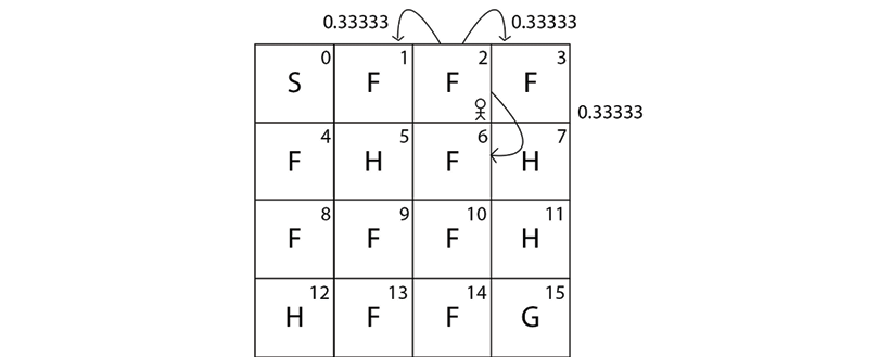
Figure 2.7: Transition probability of the agent in state 2

As we can see, in a stochastic environment we reach the next states with some probability. Now, let's learn how to obtain this transition probability using the Gym environment.

We can obtain the transition probability and the reward function by just typing env.P[state][action]. So, to obtain the transition probability of moving from state S to the other states by performing the action right, we can type env.P[S][right]. But we cannot just type state S and action right directly since they are encoded as numbers. We learned that state S is encoded as 0 and the action right is encoded as 2, so, to obtain the transition probability of state S by performing the action right, we type env.P[0][2] as the following shows:

print(env.P[0][2])

The above code will print:

[(0.33333, 4, 0.0, False),
 (0.33333, 1, 0.0, False),
 (0.33333, 0, 0.0, False)]

What does this imply? Our output is in the form of [(transition probability, next state, reward, Is terminal state?)]. It implies that if we perform an action 2 (right) in state 0 (S) then:

• We reach state 4 (F) with probability 0.33333 and receive 0 reward.
• We reach state 1 (F) with probability 0.33333 and receive 0 reward.
• We reach the same state 0 (S) with probability 0.33333 and receive 0 reward.

Figure 2.8 shows the transition probability:

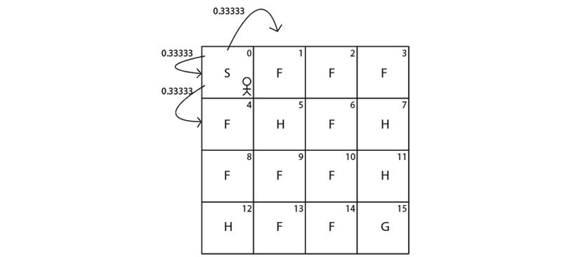
Figure 2.8: Transition probability of the agent in state 0

Thus, when we type env.P[state][action], we get the result in the form of [(transition probability, next state, reward, Is terminal state?)]. The last value is Boolean and tells us whether the next state is a terminal state. Since 4, 1, and 0 are not terminal states, it is given as false.

The output of env.P[0][2] is shown in Table 2.2 for more clarity:

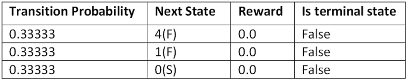
Table 2.2: Output of env.P[0][2]

Let's understand this with one more example. Let's suppose we are in state 3 (F) as Figure 2.9 shows:

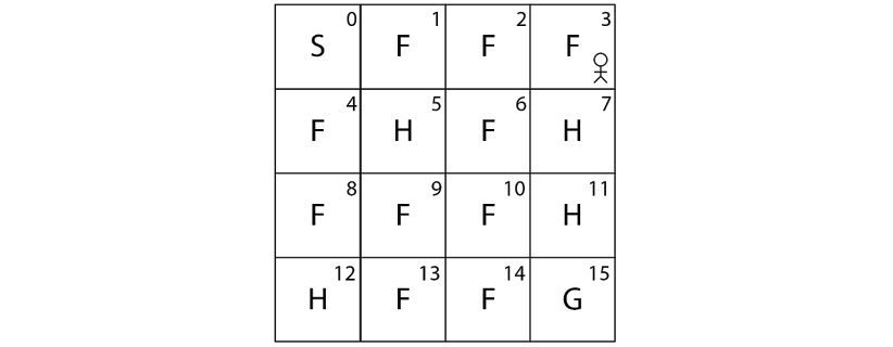
Figure 2.9: The agent in state 3

Say we perform action 1 (down) in state 3 (F). Then the transition probability of state 3 (F) by performing action 1 (down) can be obtained as the following shows:

print(env.P[3][1])

The preceding code will print:

[(0.33333, 2, 0.0, False),
 (0.33333, 7, 0.0, True),
 (0.33333, 3, 0.0, False)]

As we learned, our output is in the form of [(transition probability, next state, reward, Is terminal state?)]. It implies that if we perform action 1 (down) in state 3 (F) then:

• We reach state 2 (F) with probability 0.33333 and receive 0 reward.
• We reach state 7 (H) with probability 0.33333 and receive 0 reward.
• We reach the same state 3 (F) with probability 0.33333 and receive 0 reward.

Figure 2.10 shows the transition probability:

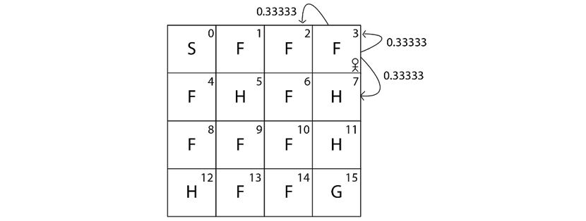
Figure 2.10: Transition probabilities of the agent in state 3

The output of env.P[3][1] is shown in Table 2.3 for more clarity:

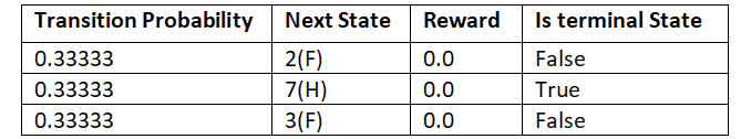
Table 2.3: Output of env.P[3][1]

As we can observe, in the second row of our output, we have (0.33333, 7, 0.0, True), and the last value here is marked as True. It implies that state 7 is a terminal state. That is, if we perform action 1 (down) in state 3 (F) then we reach state 7 (H) with 0.33333 probability, and since 7 (H) is a hole, the agent dies if it reaches state 7 (H). Thus 7(H) is a terminal state and so it is marked as True.

Thus, we have learned how to obtain the state space, action space, transition probability, and the reward function using the Gym environment. In the next section, we will learn how to generate an episode.

Generating an episode in the Gym environment

We learned that the agent-environment interaction starting from an initial state until the terminal state is called an episode. In this section, we will learn how to generate an episode in the Gym environment.

Before we begin, we initialize the state by resetting our environment; resetting puts our agent back to the initial state. We can reset our environment using the reset() function as shown as follows:

state = env.reset()

Action selection

In order for the agent to interact with the environment, it has to perform some action in the environment. So, first, let's learn how to perform an action in the Gym environment. Let's suppose we are in state 3 (F) as Figure 2.11 shows:

Figure 2.11: The agent is in state 3 in the Frozen Lake environment

Say we need to perform action 1 (down) and move to the new state 7 (H). How can we do that? We can perform an action using the step function. We just need to input our action as a parameter to the step function. So, we can perform action 1 (down) in state 3 (F) using the step function as follows:

env.step(1)

Now, let's render our environment using the render function:

env.render()

As shown in Figure 2.12, the agent performs action 1 (down) in state 3 (F) and reaches the next state 7 (H):

Figure 2.12: The agent in state 7 in the Frozen Lake environment

Note that whenever we make an action using env.step(), it outputs a tuple containing 4 values. So, when we take action 1 (down) in state 3 (F) using env.step(1), it gives the output as:

(7, 0.0, True, {'prob': 0.33333})

As you might have guessed, it implies that when we perform action 1 (down) in state 3 (F):

• We reach the next state 7 (H).
• The agent receives the reward 0.0.
• Since the next state 7 (H) is a terminal state, it is marked as True.
• We reach the next state 7 (H) with a probability of 0.33333.

So, we can just store this information as:

(next_state, reward, done, info) = env.step(1)

Thus:

• next_state represents the next state.
• reward represents the obtained reward.
• done implies whether our episode has ended. That is, if the next state is a terminal state, then our episode will end, so done will be marked as True else it will be marked as False.
• info—Apart from the transition probability, in some cases, we also obtain other information saved as info, which is used for debugging purposes.

We can also sample action from our action space and perform a random action to explore our environment. We can sample an action using the sample function:

random_action = env.action_space.sample()

After we have sampled an action from our action space, then we perform our sampled action using our step function:

next_state, reward, done, info = env.step(random_action)

Now that we have learned how to select actions in the environment, let's see how to generate an episode.

Generating an episode

Now let's learn how to generate an episode. The episode is the agent environment interaction starting from the initial state to the terminal state. The agent interacts with the environment by performing some action in each state. An episode ends if the agent reaches the terminal state. So, in the Frozen Lake environment, the episode will end if the agent reaches the terminal state, which is either the hole state (H) or goal state (G).

Let's understand how to generate an episode with the random policy. We learned that the random policy selects a random action in each state. So, we will generate an episode by taking random actions in each state. So for each time step in the episode, we take a random action in each state and our episode will end if the agent reaches the terminal state.

First, let's set the number of time steps:

num_timesteps = 20

For each time step:

for t in range(num_timesteps):

Randomly select an action by sampling from the action space:

    random_action = env.action_space.sample()

Perform the selected action:

    next_state, reward, done, info = env.step(random_action)

If the next state is the terminal state, then break. This implies that our episode ends:

    if done:
        break

The preceding complete snippet is provided for clarity. The following code denotes that on every time step, we select an action by randomly sampling from the action space, and our episode will end if the agent reaches the terminal state:

import gym
env = gym.make("FrozenLake-v0")
state = env.reset()
print('Time Step 0 :')
env.render()
num_timesteps = 20
for t in range(num_timesteps):
  random_action = env.action_space.sample()
  new_state, reward, done, info = env.step(random_action)
  print ('Time Step {} :'.format(t+1))
  env.render()
  if done:
    break

The preceding code will print something similar to Figure 2.13. Note that you might get a different result each time you run the preceding code since the agent is taking a random action in each time step.

As we can observe from the following output, on each time step, the agent takes a random action in each state and our episode ends once the agent reaches the terminal state. As Figure 2.13 shows, in time step 4, the agent reaches the terminal state H, and so the episode ends:

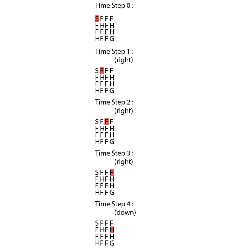
Figure 2.13: Actions taken by the agent in each time step

Instead of generating one episode, we can also generate a series of episodes by taking some random action in each state:

import gym
env = gym.make("FrozenLake-v0")
num_episodes = 10
num_timesteps = 20 
for i in range(num_episodes):
    
    state = env.reset()
    print('Time Step 0 :')
    env.render()
    for t in range(num_timesteps):
        random_action = env.action_space.sample()
        
        new_state, reward, done, info = env.step(random_action)
        print ('Time Step {} :'.format(t+1))
        env.render()
        if done:
            break

Thus, we can generate an episode by selecting a random action in each state by sampling from the action space. But wait! What is the use of this? Why do we even need to generate an episode?

In the previous chapter, we learned that an agent can find the optimal policy (that is, the correct action in each state) by generating several episodes. But in the preceding example, we just took random actions in each state over all the episodes. How can the agent find the optimal policy? So, in the case of the Frozen Lake environment, how can the agent find the optimal policy that tells the agent to reach state G from state S without visiting the hole states H?

This is where we need a reinforcement learning algorithm. Reinforcement learning is all about finding the optimal policy, that is, the policy that tells us what action to perform in each state. We will learn how to find the optimal policy by generating a series of episodes using various reinforcement learning algorithms in the upcoming chapters. In this chapter, we will focus on getting acquainted with the Gym environment and various Gym functionalities as we will be using the Gym environment throughout the course of the book.

So far we have understood how the Gym environment works using the basic Frozen Lake environment, but Gym has so many other functionalities and also several interesting environments. In the next section, we will learn about the other Gym environments along with exploring the functionalities of Gym.

In this section, we will explore several interesting Gym environments, along with exploring different functionalities of Gym.

Classic control environments

Gym provides environments for several classic control tasks such as Cart-Pole balancing, swinging up an inverted pendulum, mountain car climbing, and so on. Let's understand how to create a Gym environment for a Cart-Pole balancing task. The Cart-Pole environment is shown below:

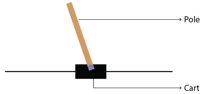
Figure 2.14: Cart-Pole example

Cart-Pole balancing is one of the classical control problems. As shown in Figure 2.14, the pole is attached to the cart and the goal of our agent is to balance the pole on the cart, that is, the goal of our agent is to keep the pole standing straight up on the cart as shown in Figure 2.15:

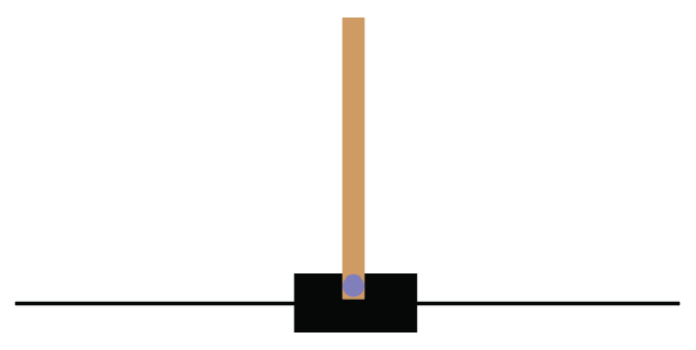
Figure 2.15: The goal is to keep the pole straight up

So the agent tries to push the cart left and right to keep the pole standing straight on the cart. Thus our agent performs two actions, which are pushing the cart to the left and pushing the cart to the right, to keep the pole standing straight on the cart. You can also check out this very interesting video, https://youtu.be/qMlcsc43-lg, which shows how the RL agent balances the pole on the cart by moving the cart left and right.

Now, let's learn how to create the Cart-Pole environment using Gym. The environment id of the Cart-Pole environment in Gym is CartPole-v0, so we can just use our make function to create the Cart-Pole environment as shown below:

env = gym.make("CartPole-v0")

After creating the environment, we can view our environment using the render function:

env.render()

We can also close the rendered environment using the close function:

env.close()

State space

Now, let's look at the state space of our Cart-Pole environment. Wait! What are the states here? In the Frozen Lake environment, we had 16 discrete states from S to G. But how can we describe the states here? Can we describe the state by cart position? Yes! Note that the cart position is a continuous value. So, in this case, our state space will be continuous values, unlike the Frozen Lake environment where our state space had discrete values (S to G).

But with just the cart position alone we cannot describe the state of the environment completely. So we include cart velocity, pole angle, and pole velocity at the tip. So we can describe our state space by an array of values as shown as follows:

array([cart position, cart velocity, pole angle, pole velocity at the tip])

Note that all of these values are continuous, that is:

1. The value of the cart position ranges from -4.8 to 4.8.
2. The value of the cart velocity ranges from -Inf to Inf ( to ).
3. The value of the pole angle ranges from -0.418 radians to 0.418 radians.
4. The value of the pole velocity at the tip ranges from -Inf to Inf.

Thus, our state space contains an array of continuous values. Let's learn how we can obtain this from Gym. In order to get the state space, we can just type env.observation_space as shown as follows:

print(env.observation_space)

The preceding code will print:

Box(4,)

Box implies that our state space consists of continuous values and not discrete values. That is, in the Frozen Lake environment, we obtained the state space as Discrete(16), which shows that we have 16 discrete states (S to G). But now we have our state space denoted as Box(4,), which implies that our state space is continuous and consists of an array of 4 values.

For example, let's reset our environment and see how our initial state space will look like. We can reset the environment using the reset function:

print(env.reset())

The preceding code will print:

array([ 0.02002635, -0.0228838 ,  0.01248453,  0.04931007])

Note that here the state space is randomly initialized and so we will get different values every time we run the preceding code.

The result of the preceding code implies that our initial state space consists of an array of 4 values that denote the cart position, cart velocity, pole angle, and pole velocity at the tip, respectively. That is:

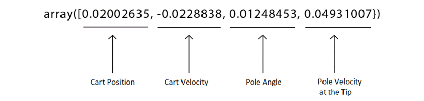
Figure 2.16: Initial state space

Okay, how can we obtain the maximum and minimum values of our state space? We can obtain the maximum values of our state space using env.observation_space.high and the minimum values of our state space using env.observation_space.low.

For example, let's look at the maximum value of our state space:

print(env.observation_space.high)

The preceding code will print:

[4.8000002e+00 3.4028235e+38 4.1887903e-01 3.4028235e+38]

It implies that:

1. The maximum value of the cart position is 4.8.
2. We learned that the maximum value of the cart velocity is +Inf, and we know that infinity is not really a number, so it is represented using the largest positive real value 3.4028235e+38.
3. The maximum value of the pole angle is 0.418 radians.
4. The maximum value of the pole velocity at the tip is +Inf, so it is represented using the largest positive real value 3.4028235e+38.

Similarly, we can obtain the minimum value of our state space as:

print(env.observation_space.low)

The preceding code will print:

[-4.8000002e+00 -3.4028235e+38 -4.1887903e-01 -3.4028235e+38]

It states that:

1. The minimum value of the cart position is -4.8.
2. We learned that the minimum value of the cart velocity is -Inf, and we know that infinity is not really a number, so it is represented using the largest negative real value -3.4028235e+38.
3. The minimum value of the pole angle is -0.418 radians.
4. The minimum value of the pole velocity at the tip is -Inf, so it is represented using the largest negative real value -3.4028235e+38.

Action space

Now, let's look at the action space. We already learned that in the Cart-Pole environment we perform two actions, which are pushing the cart to the left and pushing the cart to the right, and thus the action space is discrete since we have only two discrete actions.

In order to get the action space, we can just type env.action_space as the following shows:

print(env.action_space)

The preceding code will print:

Discrete(2)

As we can observe, Discrete(2) implies that our action space is discrete, and we have two actions in our action space. Note that the actions will be encoded into numbers as shown in Table 2.4:

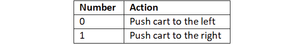
Table 2.4: Two possible actions

Cart-Pole balancing with random policy

Let's create an agent with the random policy, that is, we create the agent that selects a random action in the environment and tries to balance the pole. The agent receives a +1 reward every time the pole stands straight up on the cart. We will generate over 100 episodes, and we will see the return (sum of rewards) obtained over each episode. Let's learn this step by step.

First, let's create our Cart-Pole environment:

import gym
env = gym.make('CartPole-v0')

Set the number of episodes and number of time steps in the episode:

num_episodes = 100
num_timesteps = 50

For each episode:

for i in range(num_episodes):

Set the return to 0:

    Return = 0

Initialize the state by resetting the environment:

    state = env.reset()

For each step in the episode:

    for t in range(num_timesteps):

Render the environment:

        env.render()

Randomly select an action by sampling from the environment:

        random_action = env.action_space.sample()

Perform the randomly selected action:

        next_state, reward, done, info = env.step(random_action)

Update the return:

        Return = Return + reward

If the next state is a terminal state then end the episode:

        if done:
            break

For every 10 episodes, print the return (sum of rewards):

    if i%10==0:
        print('Episode: {}, Return: {}'.format(i, Return))
        

Close the environment:

env.close()

The preceding code will output the sum of rewards obtained over every 10 episodes:

Episode: 0, Return: 14.0
Episode: 10, Return: 31.0
Episode: 20, Return: 16.0
Episode: 30, Return: 9.0
Episode: 40, Return: 18.0
Episode: 50, Return: 13.0
Episode: 60, Return: 25.0
Episode: 70, Return: 21.0
Episode: 80, Return: 17.0
Episode: 90, Return: 14.0

Thus, we have learned about one of the interesting and classic control problems called Cart-Pole balancing and how to create the Cart-Pole balancing environment using Gym. Gym provides several other classic control environments as shown in Figure 2.17:

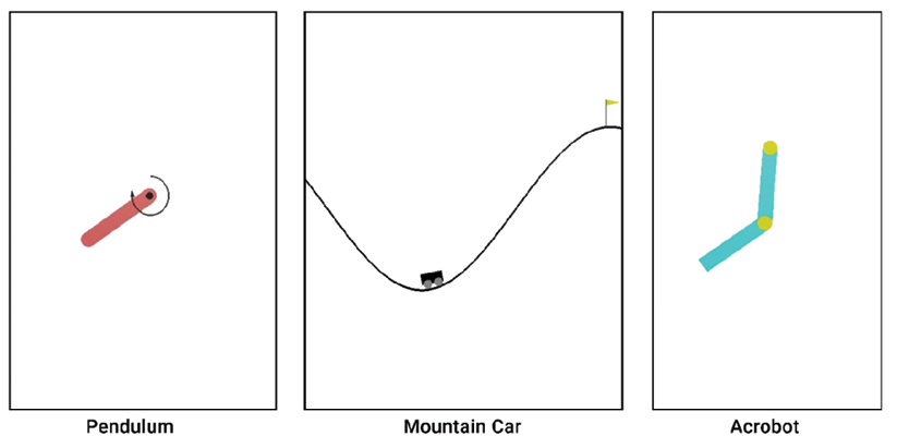
Figure 2.17: Classic control environments

You can also do some experimentation by creating any of the above environments using Gym. We can check all the classic control environments offered by Gym here: https://gym.openai.com/envs/#classic_control.

Atari game environments

Are you a fan of Atari games? If yes, then this section will interest you. Atari 2600 is a video game console from a game company called Atari. The Atari game console provides several popular games, which include Pong, Space Invaders, Ms. Pac-Man, Break Out, Centipede, and many more. Training our reinforcement learning agent to play Atari games is an interesting as well as challenging task. Often, most of the RL algorithms will be tested out on Atari game environments to evaluate the accuracy of the algorithm.

In this section, we will learn how to create the Atari game environment using Gym. Gym provides about 59 Atari game environments including Pong, Space Invaders, Air Raid, Asteroids, Centipede, Ms. Pac-Man, and so on. Some of the Atari game environments provided by Gym are shown in Figure 2.18 to keep you excited:

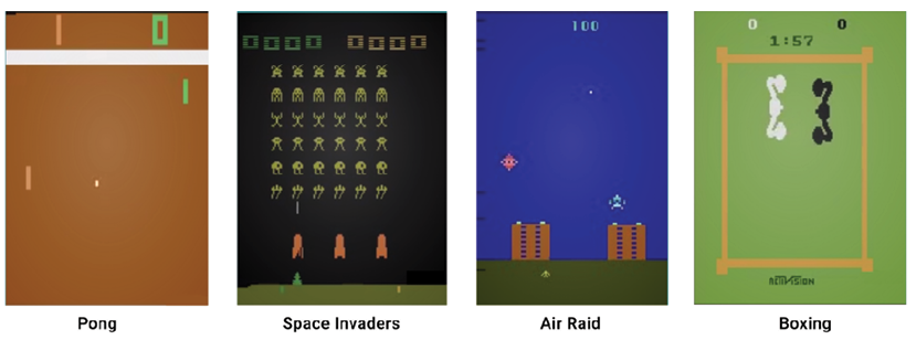
Figure 2.18: Atari game environments

In Gym, every Atari game environment has 12 different variants. Let's understand this with the Pong game environment. The Pong game environment will have 12 different variants as explained in the following sections.

General environment

• Pong-v0 and Pong-v4: We can create a Pong environment with the environment id as Pong-v0 or Pong-v4. Okay, what about the state of our environment? Since we are dealing with the game environment, we can just take the image of our game screen as our state. But we can't deal with the raw image directly so we will take the pixel values of our game screen as the state. We will learn more about this in the upcoming section.
• Pong-ram-v0 and Pong-ram-v4: This is similar to Pong-v0 and Pong-v4, respectively. However, here, the state of the environment is the RAM of the Atari machine, which is just the 128 bytes instead of the game screen's pixel values.

Deterministic environment

• PongDeterministic-v0 and PongDeterministic-v4: In this type, as the name suggests, the initial position of the game will be the same every time we initialize the environment, and the state of the environment is the pixel values of the game screen.
• Pong-ramDeterministic-v0 and Pong-ramDeterministic-v4: This is similar to PongDeterministic-v0 and PongDeterministic-v4, respectively, but here the state is the RAM of the Atari machine.

No frame skipping

• PongNoFrameskip-v0 and PongNoFrameskip-v4: In this type, no game frame is skipped; all game screens are visible to the agent and the state is the pixel value of the game screen.
• Pong-ramNoFrameskip-v0 and Pong-ramNoFrameskip-v4: This is similar to PongNoFrameskip-v0 and PongNoFrameskip-v4, but here the state is the RAM of the Atari machine.

Thus in the Atari environment, the state of our environment will be either the game screen or the RAM of the Atari machine. Note that similar to the Pong game, all other Atari games have the id in the same fashion in the Gym environment. For example, suppose we want to create a deterministic Space Invaders environment; then we can just create it with the id SpaceInvadersDeterministic-v0. Say we want to create a Space Invaders environment with no frame skipping; then we can create it with the id SpaceInvadersNoFrameskip-v0.

We can check out all the Atari game environments offered by Gym here: https://gym.openai.com/envs/#atari.

State and action space

Now, let's explore the state space and action space of the Atari game environments in detail.

State space

In this section, let's understand the state space of the Atari games in the Gym environment. Let's learn this with the Pong game. We learned that in the Atari environment, the state of the environment will be either the game screen's pixel values or the RAM of the Atari machine. First, let's understand the state space where the state of the environment is the game screen's pixel values.

Let's create a Pong environment with the make function:

env = gym.make("Pong-v0")

Here, the game screen is the state of our environment. So, we will just take the image of the game screen as the state. However, we can't deal with the raw images directly, so we will take the pixel values of the image (game screen) as our state. The dimension of the image pixel will be 3 containing the image height, image width, and the number of the channel.

Thus, the state of our environment will be an array containing the pixel values of the game screen:

 [Image height, image width, number of the channel]

Note that the pixel values range from 0 to 255. In order to get the state space, we can just type env.observation_space as the following shows:

print(env.observation_space)

The preceding code will print:

Box(210, 160, 3)

This indicates that our state space is a 3D array with a shape of [210,160,3]. As we've learned, 210 denotes the height of the image, 160 denotes the width of the image, and 3 represents the number of channels.

For example, we can reset our environment and see how the initial state space looks like. We can reset the environment using the reset function:

print(env.reset())

The preceding code will print an array representing the initial game screen's pixel value.

Now, let's create a Pong environment where the state of our environment is the RAM of the Atari machine instead of the game screen's pixel value:

env = gym.make("Pong-ram-v0")

Let's look at the state space:

print(env.observation_space)

The preceding code will print:

Box(128,)

This implies that our state space is a 1D array containing 128 values. We can reset our environment and see how the initial state space looks like:

print(env.reset())

Note that this applies to all Atari games in the Gym environment, for example, if we create a space invaders environment with the state of our environment as the game screen's pixel value, then our state space will be a 3D array with a shape of Box(210, 160, 3). However, if we create the Space Invaders environment with the state of our environment as the RAM of Atari machine, then our state space will be an array with a shape of Box(128,).

Action space

Let's now explore the action space. In general, the Atari game environment has 18 actions in the action space, and the actions are encoded from 0 to 17 as shown in Table 2.5:

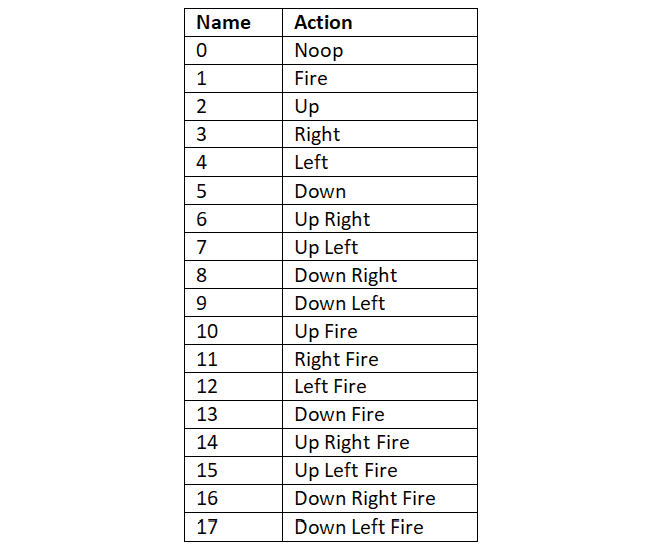
Table 2.5: Atari game environment actions

Note that all the preceding 18 actions are not applicable to all the Atari game environments and the action space varies from game to game. For instance, some games use only the first six of the preceding actions as their action space, and some games use only the first nine of the preceding actions as their action space, while others use all of the preceding 18 actions. Let's understand this with an example using the Pong game:

env = gym.make("Pong-v0")
print(env.action_space)

The preceding code will print:

Discrete(6)

The code shows that we have 6 actions in the Pong action space, and the actions are encoded from 0 to 5. So the possible actions in the Pong game are noop (no action), fire, up, right, left, and down.

Let's now look at the action space of the Road Runner game. Just in case you have not come across this game before, the game screen looks like this:

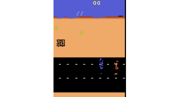
Figure 2.19: The Road Runner environment

Let's see the action space of the Road Runner game:

env = gym.make("RoadRunner-v0")
print(env.action_space)

The preceding code will print:

Discrete(18)

This shows us that the action space in the Road Runner game includes all 18 actions.

An agent playing the Tennis game

In this section, let's explore how to create an agent to play the Tennis game. Let's create an agent with a random policy, meaning that the agent will select an action randomly from the action space and perform the randomly selected action.

First, let's create our Tennis environment:

import gym
env = gym.make('Tennis-v0')

Let's view the Tennis environment:

env.render()

The preceding code will display the following:

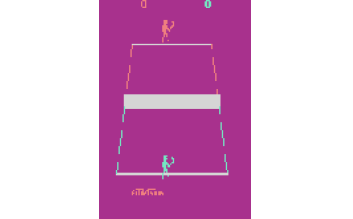
Figure 2.20: The Tennis game environment

Set the number of episodes and the number of time steps in the episode:

num_episodes = 100
num_timesteps = 50

For each episode:

for i in range(num_episodes):

Set the return to 0:

    Return = 0

Initialize the state by resetting the environment:

    state = env.reset()

For each step in the episode:

    for t in range(num_timesteps):

Render the environment:

        env.render()

Randomly select an action by sampling from the environment:

        random_action = env.action_space.sample()

Perform the randomly selected action:

        next_state, reward, done, info = env.step(random_action)

Update the return:

        Return = Return + reward

If the next state is a terminal state, then end the episode:

        if done:
            break

For every 10 episodes, print the return (sum of rewards):

    if i%10==0:
        print('Episode: {}, Return: {}'.format(i, Return))
        

Close the environment:

env.close()

The preceding code will output the return (sum of rewards) obtained over every 10 episodes:

Episode: 0, Return: -1.0
Episode: 10, Return: -1.0
Episode: 20, Return: 0.0
Episode: 30, Return: -1.0
Episode: 40, Return: -1.0
Episode: 50, Return: -1.0
Episode: 60, Return: 0.0
Episode: 70, Return: 0.0
Episode: 80, Return: -1.0
Episode: 90, Return: 0.0

Recording the game

We have just learned how to create an agent that randomly selects an action from the action space and plays the Tennis game. Can we also record the game played by the agent and save it as a video? Yes! Gym provides a wrapper class, which we can use to save the agent's gameplay as video.

To record the game, our system should support FFmpeg. FFmpeg is a framework used for processing media files. So before moving ahead, make sure that your system provides FFmpeg support.

We can record our game using the Monitor wrapper as the following code shows. It takes three parameters: the environment; the directory where we want to save our recordings; and the force option. If we set force = False, it implies that we need to create a new directory every time we want to save new recordings, and when we set force = True, old recordings in the directory will be cleared out and replaced by new recordings:

env = gym.wrappers.Monitor(env, 'recording', force=True)

We just need to add the preceding line of code after creating our environment. Let's take a simple example and see how the recordings work. Let's make our agent randomly play the Tennis game for a single episode and record the agent's gameplay as a video:

import gym
env = gym.make('Tennis-v0')
#Record the game
env = gym.wrappers.Monitor(env, 'recording', force=True)
env.reset()
for _ in range(5000):
    env.render()
    action = env.action_space.sample() 
    next_state, reward, done, info = env.step(action)
    if done:
        break
env.close()

Once the episode ends, we will see a new directory called recording and we can find the video file in MP4 format in this directory, which has our agent's gameplay as shown in Figure 2.21:

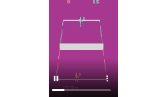
Figure 2.21: The Tennis gameplay

Other environments

Apart from the classic control and the Atari game environments we've discussed, Gym also provides several different categories of the environment. Let's find out more about them.

Box2D

Box2D is the 2D simulator that is majorly used for training our agent to perform continuous control tasks, such as walking. For example, Gym provides a Box2D environment called BipedalWalker-v2, which we can use to train our agent to walk. The BipedalWalker-v2 environment is shown in Figure 2.22:

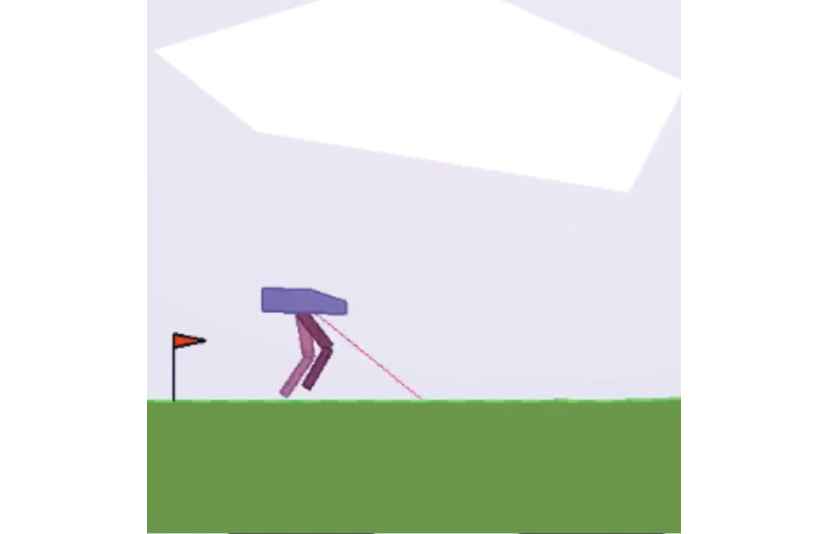
Figure 2.22: The Bipedal Walker environment

We can check out several other Box2D environments offered by Gym here: https://gym.openai.com/envs/#box2d.

MuJoCo

Mujoco stands for Multi-Joint dynamics with Contact and is one of the most popular simulators used for training our agent to perform continuous control tasks. For example, MuJoCo provides an interesting environment called HumanoidStandup-v2, which we can use to train our agent to stand up. The HumanoidStandup-v2 environment is shown in Figure 2.23:

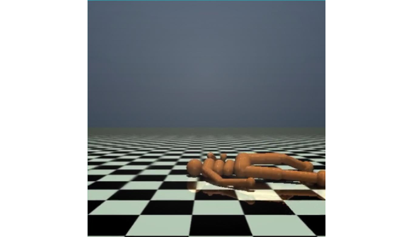
Figure 2.23: The Humanoid Stand Up environment

We can check out several other Mujoco environments offered by Gym here: https://gym.openai.com/envs/#mujoco.

Robotics

Gym provides several environments for performing goal-based tasks for the fetch and shadow hand robots. For example, Gym provides an environment called HandManipulateBlock-v0, which we can use to train our agent to orient a box using a robotic hand. The HandManipulateBlock-v0 environment is shown in Figure 2.24:

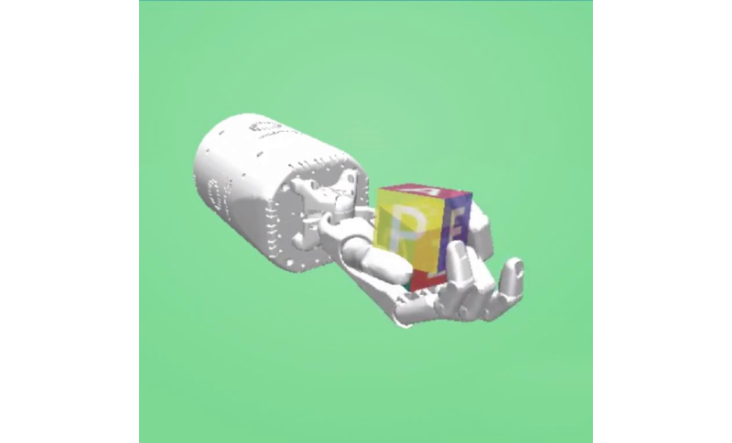
Figure 2.24: The Hand Manipulate Block environment

We can check out the several robotics environments offered by Gym here: https://gym.openai.com/envs/#robotics.

Toy text

Toy text is the simplest text-based environment. We already learned about one such environment at the beginning of this chapter, which is the Frozen Lake environment. We can check out other interesting toy text environments offered by Gym here: https://gym.openai.com/envs/#toy_text.

Algorithms

Instead of using our RL agent to play games, can we make use of our agent to solve some interesting problems? Yes! The algorithmic environment provides several interesting problems like copying a given sequence, performing addition, and so on. We can make use of the RL agent to solve these problems by learning how to perform computation. For instance, Gym provides an environment called ReversedAddition-v0, which we can use to train our agent to add multiple digit numbers.

We can check the algorithmic environments offered by Gym here: https://gym.openai.com/envs/#algorithmic.

We have learned about several types of Gym environment. Wouldn't it be nice if we could have information about all the environments in a single place? Yes! The Gym wiki provides a description of all the environments with their environment id, state space, action space, and reward range in a table: https://github.com/openai/gym/wiki/Table-of-environments.

We can also check all the available environments in Gym using the registry.all() method:

from gym import envs
print(envs.registry.all())

The preceding code will print all the available environments in Gym.

Thus, in this chapter, we have learned about the Gym toolkit and also several interesting environments offered by Gym. In the upcoming chapters, we will learn how to train our RL agent in a Gym environment to find the optimal policy.

We started the chapter by understanding how to set up our machine by installing Anaconda and the Gym toolkit. We learned how to create a Gym environment using the gym.make() function. Later, we also explored how to obtain the state space of the environment using env.observation_space and the action space of the environment using env.action_space. We then learned how to obtain the transition probability and reward function of the environment using env.P. Following this, we also learned how to generate an episode using the Gym environment. We understood that in each step of the episode we select an action using the env.step() function.

We understood the classic control methods in the Gym environment. We learned about the continuous state space of the classic control environments and how they are stored in an array. We also learned how to balance a pole using a random agent. Later, we learned about interesting Atari game environments, and how Atari game environments are named in Gym, and then we explored their state space and action space. We also learned how to record the agent's gameplay using the wrapper class, and at the end of the chapter, we discovered other environments offered by Gym.

In the next chapter, we will learn how to find the optimal policy using two interesting algorithms called value iteration and policy iteration.

Let's evaluate our newly gained knowledge by answering the following questions:

1. What is the use of a Gym toolkit?
2. How do we create an environment in Gym?
3. How do we obtain the action space of the Gym environment?
4. How do we visualize the Gym environment?
5. Name some classic control environments offered by Gym.
6. How do we generate an episode using the Gym environment?
7. What is the state space of Atari Gym environments?
8. How do we record the agent's gameplay?

Check out the following resources for more information:

• To learn more about Gym, go to http://gym.openai.com/docs/.
• We can also check out the Gym repository to understand how Gym environments are coded: https://github.com/openai/gym.