Julia is a high-level, general-purpose language that offers a fresh approach to data analysis and visualization. Its clean syntax and high performance make Julia a language worth knowing for any data scientist.

This chapter will introduce the minimum set of concepts and techniques needed for data visualization in Julia. Therefore, we will explore Julia's essential tools for representing, analyzing, and plotting data in a reproducible way. If you are starting with Julia, this chapter is vital to you. Advanced Julia users wanting to learn about the Plots package can benefit from the last section of this chapter.

After reading this chapter, you will know how to set up a Julia reproducible environment for developing your data visualization tasks. You will know how to use Julia and the Plots library to create basic plots, particularly heatmaps, scatter, bar, and line plots.

In this chapter, we're going to cover the following main topics:

• Getting started with Julia
• Installing and managing packages
• Choosing a development environment
• Knowing the basic Julia types for data visualization
• Creating basic plots

In this chapter, we will explore Julia in multiple ways. You will need a computer with an operating system and architecture supported by Julia; most 32-bit and 64-bit computers running recent versions of Linux, FreeBSD, Windows, or macOS are sufficient. You will also need a modern web browser, an internet connection, and Visual Studio Code. Once you have that, this chapter will guide you on the installation of Julia and the required packages.

Also, the code examples are available in the Chapter01 folder of the following GitHub repository: https://github.com/PacktPublishing/Interactive-Visualization-and-Plotting-with-Julia. In particular, the JuliaTypes.jl Pluto notebook has the code examples for the Knowing the basic Julia types for data visualization section and BasicPlots.jl the examples for the Creating a Basic Plot section. You will find in the same folder the static HTML version of both notebooks with the embedded outputs.

We are going to get started with Julia. This section will describe how to run Julia scripts and interact with the Julia Read-Eval-Print Loop (REPL), the command line or console used to execute Julia code interactively. But first, let's install Julia on your system.

Installing Julia

We are going to install the stable release of Julia on your system. There are many ways to install Julia, depending on your operating system. Here, we are going to install Julia using the official binaries. First, let's download the binary of Julia's Long-Term Support (LTS) release, Julia 1.6. You can install other releases, but I recommend using Julia 1.6 to ensure reproducibility of the book's examples:

1. Go to https://julialang.org/downloads/.
2. Download the binary file for the LTS release that matches your operating system (Windows, macOS, Linux, or FreeBSD) and the computer architecture bit widths (64-bit or 32-bit).

If you are a Windows user, we recommend downloading the installer. When choosing the installer, note that a 64-bit version will only work on 64-bit Windows.

If you are using Linux, you should also match the instruction set architecture of your computer processor (x86, ARM, or PowerPC). You can use the following command in your terminal to learn your architecture:

uname --all

Note that i386 on the output means you have a 32-bit x86 processor, and x86_64 indicates a 64-bit x86 processor.

The instructions that follow this step depend on your operating system, so, let's see them separately. Once you have finished, you can test your Julia installation by typing julia -v on your terminal; it should print the installed Julia version.

Linux

Installation on Linux is pretty simple; you should do the following:

1. Move the downloaded file to the place you want to install Julia.
2. Decompress the downloaded .tar.gz file. On a terminal, you can use tar -xf followed by the filename to do it.
3. Put the julia executable that is inside the bin folder of the decompressed folder on PATH. The PATH system variable contains a colon-separated list of paths where your operating system can find executables. Therefore, we need the folder containing the julia executable on that list to allow your operating system to find it. There are different ways to do that depending on the Unix shell that runs in your system terminal. We will give the instructions for Bash; if you are using another shell, please look for the corresponding instructions. You can know the shell that runs in your terminal by executing echo $0.

Using Bash, you can add the full absolute path to the bin folder to PATH in ~/.bash_profile (or ~/.bashrc) by adding the following line to that file:

export PATH="$PATH:/path/to/julia_directory/bin"

You should replace /path/to/julia_directory/bin with the full path to the bin folder containing the julia binary. The $ and : characters are required; it is easy to mess up your Bash terminal by forgetting them.

macOS

To install Julia on macOS, do the following:

1. Double-click the downloaded .dmg file to decompress it.
2. Drag the .app file to the Applications folder.
3. Put julia on PATH to access it from the command line. You can do that by creating a symbolic link to julia on /usr/local/bin – for example, if you are installing Julia 1.6, you would use this:

   ln -s /Applications/Julia-1.6.app/Contents/Resources/julia/bin/julia /usr/local/bin/julia

Windows

If you are on Windows, you should only run the installer and follow the instructions. Please note the address where Julia has been installed. You will need to put the julia executable on PATH to access Julia from the command line. The following instructions are for Windows 10:

1. Open Control Panel.
2. Enter System and Security.
3. Go to System.
4. Click on Advanced system settings.
5. Click on the Environment variables... button.
6. In the User Variables and System Variables sections, look for the Path variable and click that row.
7. Click the Edit... button of the section that has the Path variable selected.
8. Click New in the Edit environment variable window.
9. Paste the path to the julia executable.
10. Click the OK button.

Interacting with the Julia REPL

Now you have installed Julia, let's start exploring the Julia REPL or console. Let's do a simple arithmetic operation:

1. Type julia on your system terminal to open the Julia REPL. If you are using Windows, we recommend using a modern terminal as the Windows terminal.
2. Type 2 + 2 after the julia> prompt on the Julia REPL and press Enter.

Voilà! You have done your first arithmetic operation in Julia.

3. Exit the Julia REPL using one of the following options:
   • Type exit() and press Enter.
   • Press the control key (Ctrl) together with the D key on a blank line.

Now that we know the basics of interacting with the Julia REPL, let's see some of its more exciting capabilities – tab completion, support for Unicode characters, and REPL modes.

Getting help from tab completion

The Tab key is handy when working on the Julia REPL. It can speed up your code input and show you the available options in a given context. When entering a name on a current workspace, pressing the Tab key will autocomplete the name until there are no ambiguities. If there are multiple options, Julia will list the possibilities.

You can also use tab completion to get information about the expected and keyword arguments that a function can take. To get that, you need to press the Tab key after the open bracket or after a comma in the argument list. For example, you can see the list of methods for the sum function, including possible arguments and their accepted types, by typing sum( and pressing the Tab key. Note that typing sum([1, 2, 3],  and pressing the Tab key will give you a shorter list, as Julia now knows that you want to sum a vector of integers.

Last but not least, you can use tab completion to find out the field names of a given object. For example, let's see the field names of a range object:

1. Type numbers = 1:10 on the Julia REPL and press Enter. That defines the variable numbers to contain a range of integers.
2. Type numbers. and press the Tab key. Julia will autocomplete st, as the two fields of a range object start with these two letters.
3. Press the Tab key. Julia will list the field names of the range object – in this case, start and stop.
4. Type a to disambiguate and press the Tab key to autocomplete.
5. Press the Enter key to see the value of numbers.start.

Julia can autocomplete more things, such as the fields of a function output or a dictionary's keys. As we will see next, you can also use tab autocompletion to enter Unicode characters.

Unicode input

Julia allows you to use any Unicode character, including an emoji, on your variables and function names. You can copy and paste those characters from any source. Also, you can insert them using tab completion of their LaTeX-like abbreviation, starting with the \ character. For example, you can enter π by typing \pi and pressing the Tab key.

REPL modes

Julia offers a variety of REPL modes to facilitate different tasks. You can enter the different modes by pressing a specific key just after the julia> prompt. The following figure shows you the built-in REPL modes that come with Julia:

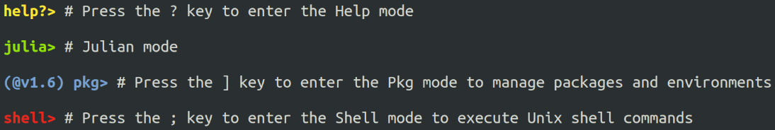
Figure 1.1 – The REPL modes

Let's test that by using the most helpful mode, the help mode to access the documentation of the split function:

1. Press the ? key just after the julia> prompt; you will see that the prompt changes to help?>.
2. Type split and press Enter; you will see the function's documentation and automatically return to the julia> prompt.

Going back to the julia> prompt only requires pressing the Backspace key just after the prompt of the REPL mode. Another way to come back to the julia> prompt is by pressing the control (Ctrl) and C keys together. In this case, we didn't need the Backspace key to return to the julia> prompt as the help mode isn't sticky. However, the shell and pkg modes shown in Figure 1.1 are sticky and require pressing the Backspace key to go out of them.

Running Julia scripts

Using the Julia REPL is helpful for interactive tasks and ephemeral code, but creating and running Julia scripts can be a better option in other situations. A Julia script is simply a text file with the jl extension containing Julia code. The easiest way to run a Julia script in your system terminal is by running the julia executable and giving the path to the script file as the first positional argument. For instance, if you want to run a Julia script named script.jl that is in the current folder, you can run the following line in the terminal:

julia script.jl

We have now installed Julia and learned how to run Julia code. In the next section, we will learn how to install Julia packages and manage project environments to ensure reproducibility.

Julia has a built-in package manager that you can use by loading the Pkg module or through pkg mode of the Julia REPL. In this section, we will learn how to use it to install packages and manage project environments.

Installing Julia packages

Julia has an increasing number of registered packages that you can easily install using the built-in package manager. In this section, we will install the Plots library as an example. Let's install Plots using the add command from Pkg mode. This way of installing packages comes in handy when working on the Julia REPL:

1. Open Julia.
2. Enter Pkg mode by pressing the ] key just after the julia> prompt.
3. Type add Plots after the pkg> prompt and press Enter.
4. Wait for the installation to finish; it can take some time.
5. Press the Backspace key to return to the julia> prompt.

Great! This has been easy, and you now have the Plots package installed. However, Pkg mode is only available to you when you are in the Julia REPL. But, if you want to install a Julia package from a non-interactive environment (for example, inside a Julia script), you will need to use the add function from the Pkg module. The Pkg module belongs to the Julia Standard Library. Thankfully, you don't need to install the packages of the Standard Library before using them. Let's try adding Plots again but using the Pkg module this time. As we have already installed the latest version of Plots, this will be fast:

1. Open Julia.
2. Import the Pkg module by typing import Pkg after the julia> prompt and pressing Enter.
3. Type Pkg.add("Plots") and press Enter.

In the last example, we used import to load the Pkg module. In the next section, we will learn some different ways in which you can load packages.

Loading packages

We need to load a package to use it within a Julia session. There are two main ways to load packages in Julia. The first one is using the import keyword followed by the module name – for example, import Pkg. As Julia packages export modules of the same name, you can also use the name of a package. When we use import in this way, Julia only brings the package's module into scope. Then, we need to use qualified names to access any function or variable from that module. A qualified name is simply the module name followed by a dot and the object name – for example, Pkg.add.

The second way to load a package is to use the using keyword followed by the module name. Julia will bring the module into scope, as well as all the names that the module exports. Therefore, we do not need to use qualified names to access their functions and variables. For instance, executing using Plots will bring the exported plot function into scope. You can still access unexported functions and variables using their qualified names.

Managing environments

A project environment defines a set of package dependencies, optionally with their versions. The Julia package manager has built-in support for them, and we can use them to create reproducible data analysis pipelines and visualizations. For example, this book's code examples use environments to allow the reproducibility of code through time and across different systems.

Julia defines project environments using two files. The first is the Project.toml file that stores the set of dependencies. The second is the Manifest.toml file that stores the exact version of all the packages and their dependencies. While the former is mandatory for any environment, the latter is optional. Luckily, we do not need to create those files manually, as we can manage the environment's packages through the package manager.

There are multiple options for dealing with project environments. One is to start julia in a given environment by using the --project argument. Usually, we want to create an environment in the folder where we are starting Julia. In those cases, we can use a dot to indicate the current working directory. Let's create an environment in the current folder containing a specific version of the Plots package:

1. Run julia --project=. in the terminal to open the Julia REPL using the project environment defined in the current working directory.
2. Press the ] key to enter Pkg mode. You will see the name of the current folder on the prompt. That's Pkg mode telling you that you are in that environment.
3. Type status and press Enter to see the content of your current environment.
4. Type add Plots@1.0.0 to install Plots version 1.0.0 in that environment.
5. Run the status command in Pkg mode again to check what is in the environment after the previous operation.
6. Press the Backspace key to return to the Julia prompt.

In the previous example, we have used the --project argument to start julia in a particular environment. If you run julia without indicating a project folder, you will use the default environment corresponding to your Julia version.

You can change between environments using the activate command. It takes the path to the project folder that contains the environment, and if you do not give any path, Julia will start the default environment of your Julia version. For example, executing activate . in Pkg mode will start the environment in the current working directory, and running activate will return the default Julia environment.

When you first activate a non-empty environment on your system, you must install all the required packages. To get all the needed packages, you should run the instantiate command of Pkg mode. For example, instantiation will be necessary if you want to use an environment created on another computer.

While Pkg mode of the Julia REPL is handy when you are working interactively, sometimes you need to manage environments inside a Julia script. In those cases, the Pkg module will be your best friend. So, let's create a Julia script that uses a particular version of Plots. First, create a file named installing_plots.jl with the following content, using any text editor:

import Pkg

Pkg.activate(temp=true)

Pkg.add(Pkg.PackageSpec(name="Plots", version="1.0.0"))

Pkg.status()

In that code, we are using the activate function of the Pkg module with temp=true to create and activate the script environment in a temporary folder. We need to use the PackageSpec type defined on the Pkg module to add a specific package version.

Now, you can run the script executing julia installing_plots.jl on your terminal. You will see that the script creates and activates a new environment in a temporal folder. Then, it installs and precompiles Plots and its dependencies. Finally, it shows that Plots version 1.0.0 was installed in the environment. The script will run a lot faster the second time because the packages are installed and precompiled on your system.

There are other Pkg commands and functions that you will find helpful when managing environments – status, to list the packages on the current project environment, update, and remove. You can see the complete list of Pkg commands in Pkg mode by typing ? and pressing the Enter key just after the pkg> prompt. Optionally, you can see extended help for each command by entering ? and the command name in Pkg mode. If you are using the Pkg module, you can access the documentation of the functions by typing Pkg. and the function name in help mode of the Julia REPL.

Now that we know how to install and manage Julia packages, let's start installing some packages to set up the different development environments we will use for Julia.

There are multiple options for developing using the Julia language. The choice of development environment depends on the task at hand. We will use three of them in this book – one Integrated Development Environment (IDE) and two notebooks. We generally use the IDE to write scripts and develop packages and applications. The notebooks allow us to perform exploratory and interactive data analysis and visualization. In this section of the book, we are going to introduce those development environments. Let's start with the IDE.

The Julia extension for VS Code

The official IDE for Julia is the Julia extension for VS Code. It provides a way to execute Julia code, search documentation, and visualize plots among many utilities. Describing all its features goes beyond the scope of this book. In this section, you will learn how to run Julia code on VS Code, but first, let's install the IDE.

Installing Julia for VS Code

To install and use the Julia extension, you will need Julia installed on your system and the julia executable on PATH. Then, you should install VS Code from https://code.visualstudio.com/. Once you have VS Code installed, you can install the Julia extension from it:

1. Click on the View menu and then on Extensions to open Extensions View.
2. Type julia in the search box at the top of Extensions View.
3. Click on the Install button of the Julia extension provided by julialang.
4. Restart VS Code once the installation has finished.

Let's now use our Julia IDE to run some code.

Running Julia on VS Code

There are multiple ways to run code using the Julia extension on VS Code. Here, we will run code blocks by pressing the Alt and Enter keys together (Alt + Enter) or entire files by pressing Shift + Enter. Let's test that with a simple Julia script:

1. Click on the File menu and then on the New File option; VS Code creates a new empty file.
2. Click on File and select the Save option.
3. Choose a location and name for your file using the jl extension (for example, first_script.jl) and click the Save button. The jl extension is crucial, as it will indicate to VS Code that you are coding in Julia.
4. Click on the JULIA button on the sidebar; it is the one with three dots, which you can see selected in Figure 1.2. It opens the workspace, documentation, and plot navigator panes of the Julia IDE.
5. Click on the first line of the empty file and type a = 2 + 2.
6. Press together the Alt and Enter keys; this will execute the code block. You will see the operation's output inlined on the file, just after the executed code block. Note that this can take some time the first time, as the Julia extension should precompile the VSCodeServer package. The Julia extension will open a Julia REPL, showing the status of the package precompilation and the result of the executed code block. After this first execution, you can also see the recently assigned a variable in the workspace pane.
7. Press Enter to create a new line and type println("Hello World").
8. Press Alt + Enter on that line to execute that code block. Now, the Julia extension only inlines a checkmark to indicate that Julia successfully ran the println function. The Julia extension uses a checkmark when the function returns nothing. The println function, by default, prints to the standard output and returns nothing. In this case, you can see Hello World printed in the Julia REPL. There is a Julia variable named ans when you run Julia interactively that holds the last object returned. You can see on the WORKSPACE pane that the ans variable contains nothing (see Figure 1.2).
9. Press the Shift and Enter keys together to execute the whole file. The Julia extension only inlines the output of the last expression of the executed file – in this case, the checkmark. Also, you will see that Julia did not print the result of the first expression on the Julia REPL. If you want to show a value when running a file, you need to print it explicitly, as we did with the "Hello World" string.
10. Save the changes by pressing the Ctrl and S keys together (Ctrl + S).

After finishing that process, your VS Code session will look similar to the one in the following figure:

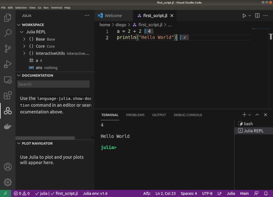
Figure 1.2 – The Julia extension for VS Code

At this point, you have set up VS Code to work with Julia on your computer, and you have learned how to run Julia code on it. This will come in handy when developing Julia scripts, packages, and applications. Also, you can now use VS Code anytime a text editor is required throughout this book. In the following section, we will learn how to execute code using Julia notebooks.

Using Julia notebooks

Notebooks are an excellent way to do literate programming, embedding code, Markdown annotations, and results into a single file. Therefore, they help to share results and ensure reproducibility. You can also code interactively using Julia notebooks instead of the Julia REPL. There are two main notebooks that you can use for Julia – Jupyter and Pluto. We are going to describe them in the following sections.

Taking advantage of Jupyter notebooks through IJulia

Jupyter notebooks are available for multiple programming languages. In Julia, they are available thanks to the IJulia package. Let's create our first Jupyter notebook:

1. Copy and paste the following code block into the Julia REPL:

   import Pkg
   Pkg.add("IJulia")

This will install the IJulia package needed for using Jupyter with Julia.

2. Type using IJulia in the Julia REPL and press Enter to load the package.
3. Now, type notebook(dir=".") and press Enter to open Jupyter. Because we set the dir keyword argument to ".", Jupyter will use the same current working directory as the Julia REPL. If this is the first time that you have run the notebook function, Julia will ask you to install Jupyter using the Conda package. You can press Enter to allow Julia to install Jupyter using a Miniconda installation private to Julia. Note that the process is automatic, but it will take some time. If you prefer using an already installed Jupyter instance instead, please read the IJulia documentation for instructions. Once Jupyter is installed, the notebook function of the IJulia package will open a tab in your web browser with Jupyter on it.
4. Go to the browser tab that is running the Jupyter frontend.
5. Click the New button on the right and select the Julia version you are using; this will open a new tab with a Julia notebook named Untitled stored in the current directory with the name Untitled.ipynb.
6. Click on Untitled and change the name of the notebook – for example, if you rename the notebook to FirstNotebook, Jupyter renames the file to FirstNotebook.ipynb.
7. Click on the empty cell and type a = 2 + 2, and then press Shift + Enter to run it. You will see that Jupyter shows the output of the expression just after the cell. The cursor moves to a new cell; in this case, as there was no cell, Jupyter creates a new one below. Note that Jupyter keeps track of the execution order by enumerating the cells' inputs (In) and outputs (Out).
8. Type println("Hello World") in the new cell and press Shift + Enter to run that code. You will see the output of the println function below the cell code. As println returns nothing, there is no numbered output for this cell (see Figure 1.3).

Jupyter supports Markdown cells to introduce formatted text, images, tables, and even LaTeX equations in your notebooks. To create them, you should click on an empty cell and then on the drop-down menu that says Code and select the Markdown option. You can write Markdown text on that cell, and Jupyter will render it when you run it (Shift + Enter). You can see an example of running **Markdown** *cell* in the following figure:

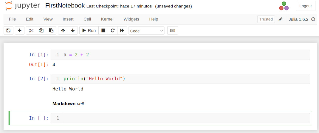
Figure 1.3 – A Jupyter notebook using Julia

In these examples, we have used one line of code for each cell, but you can write as many lines of code as you want. However, if there are multiple code blocks inside a cell, Jupyter only shows the output of the last expression. You can suppress the output of a cell by ending it with a semicolon. That trick also works on the Julia REPL and in Pluto notebooks.

Finally, you can close Jupyter by going back to the Julia terminal that runs it and pressing Ctrl + C. Jupyter autosaves the changes every 120 seconds, but if you want to save changes manually before exiting, you need to click on the save icon, the first on the toolbar, or press Ctrl + S. Now that we've had our first experience with Jupyter, let's move on to Pluto.

Using Pluto notebooks

Pluto notebooks are only available for the Julia language, and they differ from Jupyter notebooks in many aspects. One of the most important is that Pluto notebooks are reactive; that means that changing the code of one cell can trigger the execution of the dependent cells. For example, if one cell defines a variable and the second cell does something with its value, changing the variable's value in the first one will trigger the re-execution of the second. To install Pluto, you only need to install the Pluto package. Once you have installed it, let's create a new Pluto notebook:

1. Type import Pluto on the Julia REPL and press Enter.
2. Type Pluto.run() and press Enter. The run function will open Pluto in a tab in your web browser.
3. Click on the New notebook link. It will redirect you to an empty Pluto notebook.
4. Click on Save notebook... at the top middle and type a name for the notebook; it should have the jl extension – for example, FirstNotebook.jl.
5. Press Enter or click the Choose button. Pluto will create a new notebook file on the indicated path.
6. Select the empty cell, type name = "World", and press Ctrl + Enter. This will run the cell and add a new cell below. You will see that Pluto shows the cell output over the cell code.
7. Type "Hello $name" in the new cell and press Shift + Enter to execute the cell. You will see the "Hello World" string appear over the cell. The executed code creates a string by interpolating the value of the name variable.
8. Double-click on the word World in the first cell to select it and type the word Pluto.
9. Press Shift + Enter to run the cell, changing the value of the name from the "World" string to "Pluto". You will see that Pluto automatically executes the last cell, changing its output to "Hello Pluto".

Excellent! You have now had a first taste of what a reactive notebook is. Let's see how we can create a Markdown cell in Pluto:

1. Hover the mouse over the last cell; you will see that two plus symbols, +, appear over and below the cell (see Figure 1.4).
2. Click on the + symbol below the last cell to create a new cell below.
3. Type md"**Markdown** *cell*" into the new cell and press Shift + Enter to run the cell and render the Markdown string. md"" created a single-line Markdown string.
4. Hover the mouse over the cell that contains the Markdown string; you will see an eye symbol that appears on the left of the cell.
5. Click on the eye button to hide the cell code; note that Pluto has crossed out the eye icon.

There you have it! As you can see, a Markdown cell in Pluto is simply a cell that contains a Markdown string and for which we have decided not to show its source code. You can see the result of this process in the next figure:

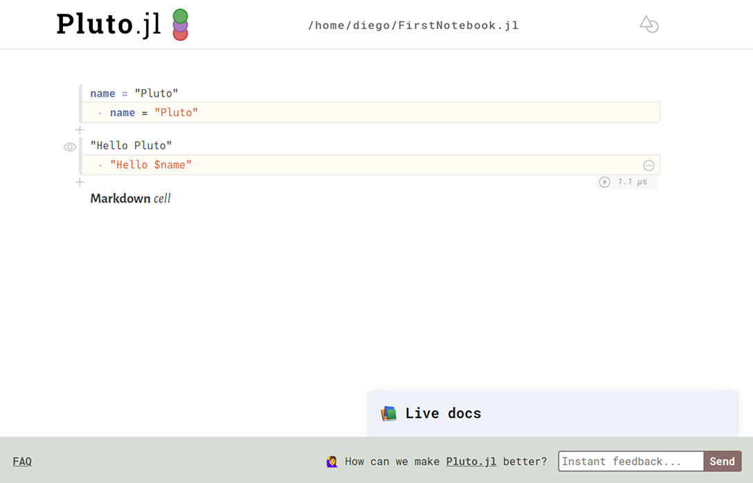
Figure 1.4 – A Pluto notebook

Pluto also differs from Jupyter by the fact that each cell should preferably do one thing. Therefore, if you plan to write multiple lines inside a single cell, they must belong to a single code block – for example, you can use multiple lines inside a function body, or a block defined between the begin and end keywords. Another difference is that Pluto doesn't allow the definition of the same variable name, nor the load of the same module in multiple cells.

Pluto notebooks are Julia files using the jl extension. You can read a Pluto notebook like any other Julia file and run it as a script. Most of the things encoding for notebook-specific aspects are just comments on the code. The outputs and figures are not stored in the file but recreated each time we open a notebook.

The best way to conserve and share code and results is to export the static HTML page. You can achieve that by clicking on the export button, a triangle over a circle located in the top-right corner of the notebook, and selecting the Static HTML option. The exported HTML also has the Julia notebook file encoded inside. This allows you to download the notebook using the Edit or run this notebook button that appears on the downloaded HTML document. There, you need to click on the notebook.jl link in the Download the notebook item in the On your computer section to download the notebook file to your machine. Then, you follow the instructions in the On your computer section to open the notebook using Pluto.

One unique aspect of Pluto notebooks that ensures reproducibility is that the notebook file also stores the project environment of the notebook. Pluto manages the notebook environment depending on the import and using statements. For example, loading a package will automatically install it in the notebook environment. If you need it, you can use the activate function of the Pkg module to disable that feature and manage the project environment yourself.

We have not used the println function in the Pluto examples because Pluto doesn't show things printed to stdout on the notebook. Instead, you can find the printed elements on the Julia REPL that is running Pluto. If you need to print something in the notebook, you will need the Print function from the PlutoUI package.

Pluto has a documentation panel that can show you the docstrings of the function and objects you are using. To open it, you need to click on the Live Docs button at the bottom right. Then, if you click on an object, for example, the Print function, you will see its documentation on the panel.

Pluto saves changes on a cell every time it runs. A Ctrl + S button at the top right will remind you to keep any unsaved changes. You can click on it or press Ctrl + S to save the changes. To close Pluto, do the following:

1. Click on the Pluto.jl icon to return to the Pluto main page.
2. Click on the dark x button at the side of the open notebooks in the Recent sessions section to close the notebooks.
3. Close the open Pluto tabs of your web browser.
4. Go to the Julia terminal that is running Pluto and press Ctrl + C to close it.

Now you know the basics of working with the three primary development environments for Julia.

Running examples using prompt pasting

Julian mode of the Julia REPL and Pluto notebooks has a nice feature called prompt pasting. It means that you can copy and paste Julia code examples, including the julia> prompt and the outputs. Julia will strip out those, leaving only the code for its execution.

In the Julia REPL, you need to paste everything after the julia> prompt; you will see that Julia automatically extracts and executes the code. In Pluto, click on a cell and paste it. You will see that Pluto pastes the code on new cells under the selected cell without running it. You should note that prompt pasting doesn't work on the standard Windows Command Prompt, nor in Jupyter.

Now you know that if you see code examples starting with the julia> prompt in this book or elsewhere, you can copy and paste them in the Julia REPL or Pluto to execute them.

This section will explore the Julia syntax, objects, and features that will help us perform data analysis and visualization tasks. Julia and its ecosystem define plenty of object types useful for us when creating visualizations. Because user-defined types are as fast as built-in types in Julia, you are not constrained to using the few structs defined in the language. This section will explore both the built-in and package-defined types that will help us the most throughout this book. But first, let's see how to create and use Julia functions.

Defining and calling functions

A function is an object able to take an input, execute some code on it, and return a value. We have already called functions using the parenthesis syntax – for example, println("Hello World"). We pass the function input values or arguments inside the parentheses that follow the function name.

We can better understand Julia's functions by creating them on our own. Let's make a straightforward function that takes two arguments and returns the sum of them. You can execute the following code in the Julia REPL, inside a new Julia script in VS Code, or into a Jupyter or Pluto cell:

function addition(x, y)

    x + y

end

We can use the function keyword to create a function. We then define its name and declare inside the parentheses the positional and keyword arguments. In this case, we have defined two positional arguments, x, and y. After a new line, we start the function body, which determines the code to be executed by the function. The function body of the previous code contains only one expression – x + y. A Julia function always returns an object, and that object is the value of the last executed expression in the function body. The end keyword indicates the end of the function block.

We can also define the function using the assignation syntax for simple functions such as the previous one, containing only one expression – for example, the following code creates a function that returns the value of subtracting the value of y from x:

subtraction(x, y) = x - y

A Julia function can also have keyword arguments defined by name instead of by position – for example, we used the dir keyword argument when we executed notebook(dir="."). When declaring a function, we should introduce the keyword arguments after a semicolon.

Higher-order functions

Functions are first-class citizens in the Julia language. Therefore, you can write Julia functions that can have other functions as inputs or outputs. Those kinds of functions are called higher-order functions. One example is the sum function, which can take a function as the first argument and apply it to each value before adding them. You can execute the following code to see how Julia takes the absolute value of each number on the vector before adding them:

sum(abs, [-1, 1])

In this example, we used a named function, abs, but usually, the input and output functions are anonymous functions.

Anonymous functions

Anonymous functions are simply functions without a user-defined name. Julia offers two foremost syntaxes to define them, one for single-line functions and the others for multiline functions. The single-line syntax uses the -> operator between the function arguments and its body. The following code will perform sum(abs, [-1, 1]), using this syntax to create an anonymous function as input to sum:

sum(x -> abs(x), [-1, 1])

The other syntax uses the do block to create an anonymous function for a higher-order function, taking a function as the first argument. We can write the previous code in the following way using the do syntax:

sum([-1, 1]) do x

    abs(x)

end

We indicated the anonymous function's arguments after the do keyword and defined the body after a new line. Julia will pass the created anonymous function as the first argument of the higher-order function, which is sum in this case.

Now that we know how to create and call functions, let's explore some types in Julia.

Working with Julia types

You can write Julia types using their literal representations. We have already used some of them throughout the chapter – for example, 2 was an integer literal, and "Hello World" was a string literal. You can see the type of an object using the typeof function – for example, executing typeof("Hello World") will return String, and typeof(2) will return Int64 in a 64-bit operating system or Int32 in a 32-bit one.

In some cases, you will find the dump function helpful, as it shows the type and the structure of an object. We recommend using the Dump function from the PlutoUI package instead, as it works in both Pluto and the Julia REPL – for example, if we execute numbers = 1:5 and then the Dump(numbers) integer literal, we will get the following output in a 64-bit machine:

UnitRange{Int64}

  start: Int64 1

  stop: Int64 5

So, Dump shows that 1:5 creates UnitRange with the start and stop fields, each containing an integer value. You can access those fields using the dot notation – for example, executing numbers.start will return the 1 integer.

Also, note that the type of 1:5 was UnitRange{Int64} in this example. UnitRange is a parametric type, for which Int64 is the value of its type parameter. Julia writes the type parameters between brackets following the type name.

Julia has an advanced type system, and we have learned the basics to explore it. Before learning about some useful Julia types, let's explore one of the reasons for Julia's power – its use of multiple dispatch.

Taking advantage of Julia's multiple dispatch

We have learned how to write functions and to explore the type of objects in Julia. Now, it's time to learn about methods. The functions we have created previously are known as generic functions. As we have not annotated the functions using types, we have also created methods for those generic functions that, in principle, can take objects of any type. You can optionally add type constraints to function arguments. Julia will consider this type annotation when choosing the most specific function method for a given set of parameters. Julia has multiple dispatch, as it uses the type information of all positional arguments to select the method to execute. The power of Julia lies in its multiple dispatch, and plotting packages take advantage of this feature. Let's see what multiple dispatch means by creating a function with two methods, one for strings and the other for integers:

1. Open a Julia REPL and execute the following:

   concatenate(a::String, b::String) = a * b

This code creates a function that concatenates two string objects, a and b. Note that Julia uses the * operator to concatenate strings. We need to use the :: operator to annotate types in Julia. In this case, we are constraining our function to take only objects of the String type.

2. Run concatenate("Hello", "World") to test that our function works as expected; it should return "HelloWorld".
3. Run methods(concatenate) to list the function's methods. You will see that the concatenate function has only one method that takes two objects of the String type – concatenate(a::String, b::String).
4. Execute concatenate(1, 2). You will see that this operation throws an error of the MethodError type. The error tells us that there is no method matching concatenate(::Int64, ::Int64) if we use a 64-bit machine; otherwise, you will see Int32 instead of Int64. The error is thrown because we have defined our concatenate to take only objects of the String type.
5. Execute concatenate(a::Int, b::Int) = parse(Int, string(a) * string(b)) to define a new method for the concatenate function taking two objects of the Int type. The function converts the input integer to strings before concatenation using the string function. Then, it uses parse to get the integer value of the Int type from the concatenated strings.
6. Run methods(concatenate); you will see this time that concatenate has two methods, one for String objects and the other for integers.
7. Run concatenate(1, 2). This time, Julia will find and select the concatenate method taking two integers, returning the integer 12.

Usually, converting types will help you to fix MethodError. When we found the error in step 4 we could have solved it by converting the integers to strings on the call site by running concatenate(string(1), string(2)) to get the "12" string. There are two main ways to convert objects in Julia explicitly – the first is by using the convert function, and the other is by using the type as a function (in other words, calling the type constructor). For example, we can convert 1, an integer, to a floating-point number of 64 bits of the Float64 type using convert(Float64, 1) or Float64(1) – which option is better will depend on the types at hand. For some types, there are special conversion functions; strings are an example of it. We need the string function to convert 1 to "1", as in string(1). Also, converting a string containing a number to that number requires the parse function – for example, to convert "1" to 1, we need to call parse(Int, "1").

At this point, we know the basics for dealing with Julia types. Let's now explore Julia types that will help us create nice visualizations throughout this book.

Representing numerical values

The most classic numbers that you can use are integers and floating-point values. As Julia was designed for scientific computing, it defines number types for different word sizes. The most used ones are Float64, which stores 64-bit floating-point numbers, and Int. This is an alias of Int64 in 64-bit operating systems or Int32 in 32-bit architectures. Both are easy to write in Julia – for example, we have already used Int literals such as -1 and 5. Then, each time you enter a number with a dot, e, or E, it will define Float64 – for example, 1.0, -2e3, and 13.5E10 are numbers of the Float64 type. The dot determines the location of the decimal point and e or E the exponent. Note that .1 is equivalent to 0.1 and 1. is 1.0, as the zero is implicit on those expressions. Float64 has a value to indicate something that is not a number – NaN. When entering numbers in Julia, you can use _ as a digit separator to make the number more legible – for example, 10_000. Sometimes, you need to add units to a number to make it meaningful. In particular, we will use mm, cm, pt, and inch from the Measures package for plotting purposes. After loading that package, write the number followed by the desired unit, for example, 10.5cm. That expression takes advantage of Julia's numeric literal coefficients. Each time you write a numeric literal, such as 10.5, just before a Julia parenthesized expression or variable, such as the cm object, you imply a multiplication. Therefore, writing 10.5cm is equivalent to writing 10.5 * cm; both return the same object.

Representing text

Julia has support for single and multiline string literals. You can write the former using double quotes (") and the latter using triple double quotes ("""). Note that Julia uses single quotes (') to define the literal for single characters of the Char type.

Julia offers other kinds of strings that will be useful for us when creating plots and interactive visualizations – Markdown, HTML, and LaTeX strings. The three of them use Julia's string macros, which you can write by adding a short word before the first quotes – md for Markdown, html for HTML, and L for LaTeX. You will need to load the Markdown standard library to use the md string macro and the LaTeXStrings external package for the L string macro. Note that Pluto automatically loads the Markdown module, so you can use md"..." without loading it. Also, Pluto renders the three of them nicely:

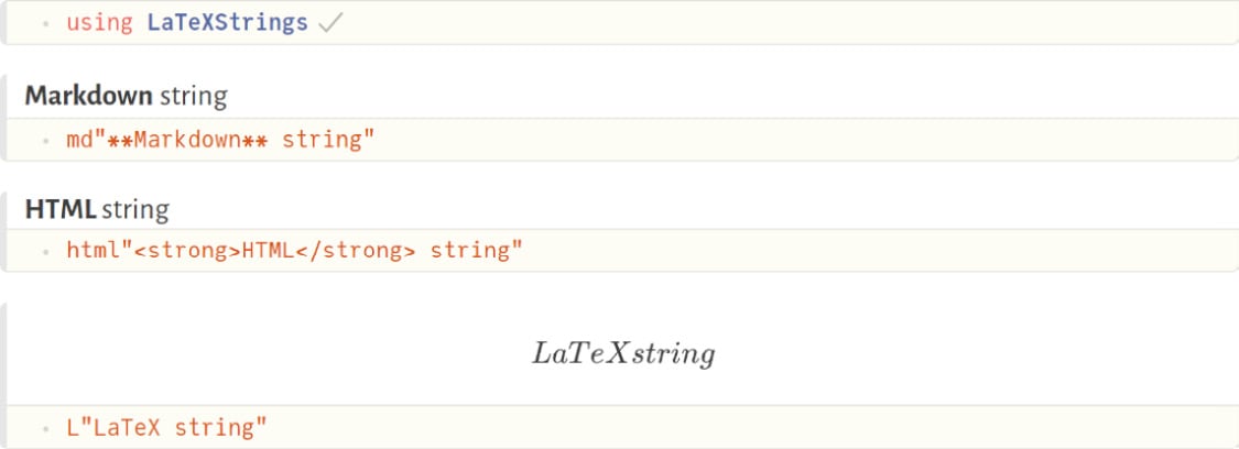
Figure 1.5 – Pluto rendering Markdown, HTML, and LaTeX strings

There is another type associated with text that you will also find in Julia when plotting and analyzing data – symbols. Symbols are interned strings, meaning that Julia stores only one copy of them. You can construct them using a colon followed by a word that should be a valid Julia variable name – for example, :var1. Otherwise, if it is not a valid identifier, you should use String and call the Symbol constructor – for example, Symbol("var1").

Working with Julia collections

We will use two main collection types for data analysis and visualization – tuples and arrays. Julia collections are a broad topic, but we will explore the minimum necessary here. Let's begin with tuples. Tuples are immutable lists of objects of any type that we write between parentheses – for example, ("x", 0) and (1,) are two- and one-element tuples respectively. Note that tuples with one element need the trailing comma.

Arrays can have multiple dimensions; the most common are vectors (one-dimensional arrays) and matrices (two-dimensional arrays). An array is a parametric type that stores the type of elements it contains and the number of dimensions as type parameters. We can construct an array using square brackets – for example, [1] and [1, 2] are vectors with one and two elements respectively. You can also write matrices using square brackets by separating columns with spaces, rather than commas and rows with semicolons or newlines – for example, [1 2; 3 4] is a 2 x 2 matrix.

For arrays, there are also other helpful constructors – zeros, ones, and rand. The three of them take the number of elements to create in each direction – for example, zeros(4, 2) will create a matrix full of zeros with four rows and two columns, while zeros(10) will create a vector of 10 zeros.

Julia offers the colon operator for creating a range of numbers; you can think of them as lazy vectors – for example, we have already seen 1:5 in a previous example. You can collect the elements of a range into a vector using the collect function.

You can index ranges, tuples, and arrays using the squared brackets syntax. Note that Julia has one-based indexing, so the first element of collection will be collection[1].

You can also iterate over ranges, tuples, and arrays. There are two compact ways to iterate through those collections, apply a function, and get a new array. One is using array comprehension – for example, [sqrt(x) for x in 1:5]. Note that comprehension can also have filter expression – for example, if we want the square root only of odd numbers between 1 and 10, we can write [sqrt(x) for x in 1:10 if x % 2 != 0] .

The other compact way to apply a function over each collection element is to use broadcasting. Julia's broadcasting allows applying a function element-wise on arrays of different sizes by expanding singleton dimensions to match their sizes. It also enables operations between scalars and collections. Furthermore, you can use broadcasting to apply a function to a single collection. Note that for each function acting on scalars, Julia doesn't define methods taking collections of them. Therefore, Julia's preferred way to apply such a function to each collection element is to use the dot syntax for broadcasting. You only need to add a dot between the function name and the parentheses on a function call or a dot before an operator – for example, sqrt.(collection) .+ 1. Julia fuses the operations when using this syntax, so the square root and the addition happen in a single iteration.

We have now learned how to work with Julia types, particularly to represent text and numbers and their collections. In the next section, we will use them to create some plots.

In the previous sections, we have learned some essentials about Julia. In this last section, we will learn how to use Julia for the creation of basic plots. For now, we will use the Plots package and its default backend, GR, but we are going to explore more deeply the Julia plotting ecosystem in the next chapter.

Let's start exploring the Plots syntax by creating a line plot, the default plot type. Line plots represent a series of related points by drawing a straight line between them.

The plot function of the Plots package can take different inputs. Plots usually take data from the positional arguments and attributes that modify the plot in the keyword arguments. The most common way to pass a series of data points is by giving their coordinates using two different vectors or ranges, one for x and the other for y. Let's do our first plot; you can choose whatever development environment you want to follow these steps:

1. Let's create some data by running the following code in the Julia REPL:

   x = 0:10
   y = sqrt.(x)

2. Run using Plots to load the Plots package.
3. Execute plot(x, y) to create your first line plot. Depending on the development environment, the plot will appear in different ways – in a new window for the Julia REPL, in the plot pane for VS Code, or inline inside the notebook for Jupyter and Pluto. You will see a plot like the one in the following figure:

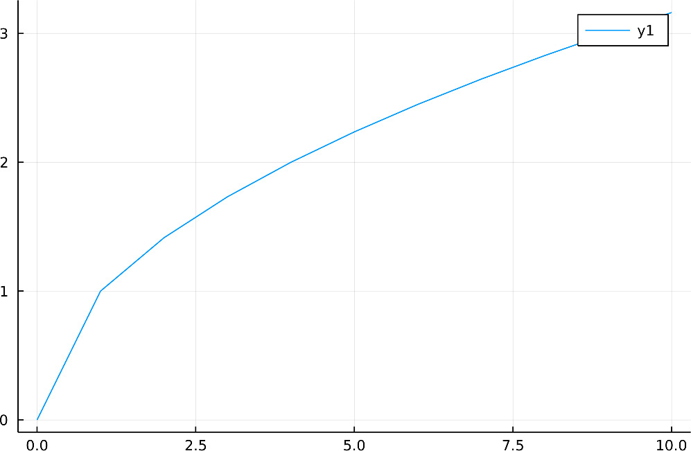
Figure 1.6 – A line plot

Great, you now have your first Julia plot! It is nice, but as we only took a few points from the sqrt function, the line has some sharp edges, most noticeably around x equal to one. Thankfully, Plots offers a better way to plot functions that adapts the number of points based on the function's second derivative. To plot a function in this way, you only need to give the function as the first argument and use the second and third positional arguments to indicate the initial and last values of x respectively – for example, to create a smooth line, the previous example becomes the following:

plot(sqrt, 0, 10)

Note that you can use your x coordinates by providing them as the second positional argument. That avoids calculating the optimal grid, so plot(sqrt, x) creates a plot identical to the first one shown in Figure 1.6.

If you give two functions as the first arguments and a domain or vector, Plots will use the latter as input for each function, and the first function will calculate the coordinates of x and the second function the coordinates of y – for example, you can define a unit circle using an angle in radians, from zero to two times pi, by defining x as the cosine of the angle and y as its sine:

plot(cos, sin, 0, 2pi, ratio=:equal)

Note that this code uses the ratio keyword argument, to ensure that we see a circle. Also, we have used Julia's numeric literal coefficient syntax to multiply 2 by the pi constant. The resulting plot is as follows:

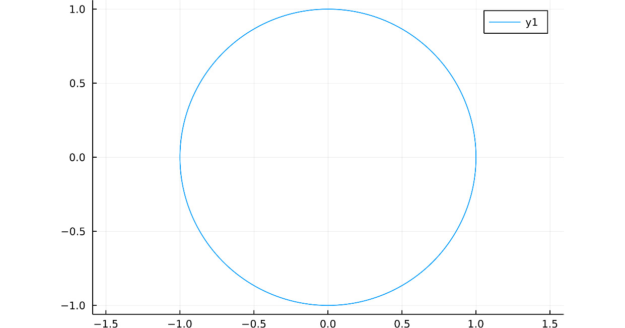
Figure 1.7 – A unit circle

In the last example, we indicated the limits of the domain, but as we said, we can also use a vector or range. For instance, try running the following:

angles = range(0, 2pi, length=100)

plot(cos, sin, angles, ratio=:equal)

In this case, we created a range using the range function to indicate the number of points we want in the plot with the length keyword argument.

We have just seen multiple ways to plot a single line, from specifying its points to using a function to let it determine them. Let's now see how to create a single plot with various lines.

Plotting multiple series

In the previous examples, we have plotted only one data series per plot. However, Plots allows you to superpose multiple series with different attributes into each plot. The main idea is that each column, vector, range, or function defines its series. For example, let's create a plot having two series, one for the sin function and the other for the cos function, using these multiple ways:

1. Define the values for the x axis, running X = range(0, 2pi, length=100).
2. Execute plot([sin, cos], X). Here, we have used a vector containing the two functions as the first argument. Each function on the vector defines a series with different labels and colors. Note that both series use the same values for the x axis.
3. Run plot(X, [sin.(X), cos.(X)]). You will get the same plot; however, we have used different inputs. The first positional argument is the range that indicates the coordinates for x. The second argument is a vector of vectors, as sin.(X), for example, uses the dot broadcasting syntax to return a vector, with the result of applying the sin function to each element of X.
4. Execute the following commands:

   Y = hcat(sin.(X), cos.(X))
   plot(X, Y)

Note that Y is now a matrix with 100 rows and 2 columns. We are using the hcat function to concatenate the two vectors resulting from the broadcasting operations. As we said, each column defines a series. The resulting plot appears in the following figure and should be identical to the previous ones:

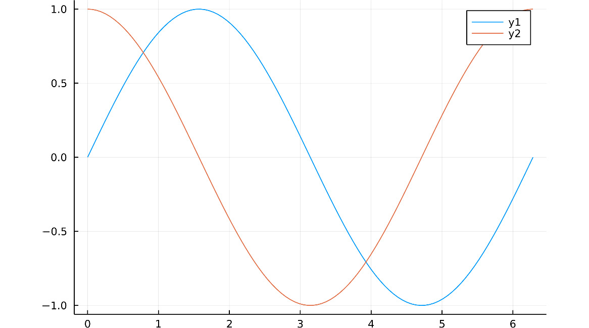
Figure 1.8 – A plot of the two data series

In Plots, each column defines a series, as in the last example. When one dimension represents multiple series, Plots repeats the dimension, having only one vector or range to match the series. That's the reason why we didn't need a matrix for x also in those examples.

Let's see how to apply different attributes to each series. In Plots, attributes indicated as vectors apply to a single series, while those defined through matrices apply to multiple ones – for example, the following code creates the plot in Figure 1.9:

plot([sin, cos], 0:0.1:2pi, 

labels=["sin" "cos"],

linecolor=[:orange :green],

linewidth=[1, 5])

Here, we are using the x-axis domain values from 0 to 2pi, with a step distance of 0.1 units. ["sin" "cos"] defines a matrix with one row and two columns, as spaces rather than commas separate the elements. We can see in Figure 1.9 that the labels attribute has assigned, for example, the string on the first column as the label of the first series. The same happens with linecolor, as we have also used a two-column matrix for it. On the contrary, [1, 5] defines a vector with two elements, and Plots has applied the same vector as the linewidth attribute of each series. So, both lines are getting a thin segment followed by a thick one. Because the number of elements in the vector given to linewidth is lower than the number of line points, Plots warns about this attribute value. The following figure shows the rendered plot:

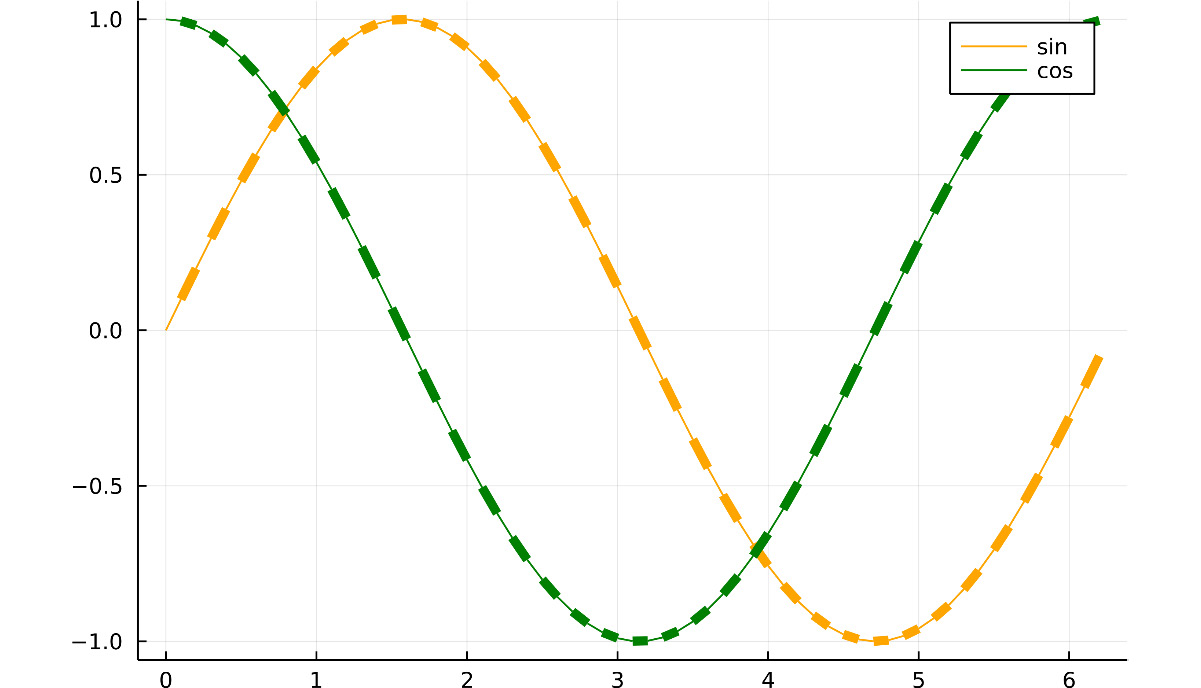
Figure 1.9 – Different series attributes

We have learned how to create multiple series in a single plot using matrix columns and a vector of vectors, ranges, or functions. While the examples only showed line plots, you can do the same for scatter and bar plots, among others. Before introducing other plots types, let's see how to add a data series to a previously created plot.

Modifying plots

Another way to add series to a plot is by modifying it using bang functions. In Julia, function names ending with a bang indicate that the function modifies its inputs. The Plots package defines many of those functions to allow us to modify previous plots. Plots' bang functions are identical to those without the bang, but they take the plot object to modify as the first argument. For example, let's create the same plot as Figure 1.8 but this time using the plot! function to add a series:

1. Execute plt = plot(sin, 0, 2pi) to create the plot for the first series and store the resulting plot object in the plt variable.
2. Run plot!(plt, cos) to add a second series for the cos function to plt. This returns the modified plot, which looks identical to the one in Figure 1.8.

If we do not indicate the plot object to modify as the first argument of a Plots bang function, Plots will change the last plot created. So, the previous code should be equivalent to running plot(sin, 0, 2pi) and then plot!(cos). However, this feature can cause problems with Pluto reactivity. So, throughout this book, we will always make explicit which plot object we want to modify.

Here, we have used the plot! function to add another line plot on top of a preexistent one. But the Plots package offers more bang functions, allowing you, for example, to add different plots types in a single figure. We will see more of these functions throughout the book. Now, let's see what other basic plot types the Plots package offers.

Scatter plots

We have created line plots suitable for representing the relationship between continuous variables and ordered points. However, we sometimes deal with points without a meaningful order, where scatter plots are a better option. There are two ways to create scatter plots with Plots – using the plot function and the seriestype attribute, or using the scatterplot function.

The default seriestype for Plots is :path, which creates the line plots. You can check that by running default(:seriestype), which returns the default value of a given attribute, written as a symbol. But we can set seriestype to :scatter to create a scatter plot – for example, let's plot the sin function using a scatter plot:

plot(sin, 0, 2pi, seriestype=:scatter)

Most of the series types define a shorthand function with the same name and the corresponding bang function – in this case, the scatter and scatter! functions. The following code produces the same plot as the previous one, using the seriestype attribute:

scatter(sin, 0, 2pi)

The resulting plot is as follows:

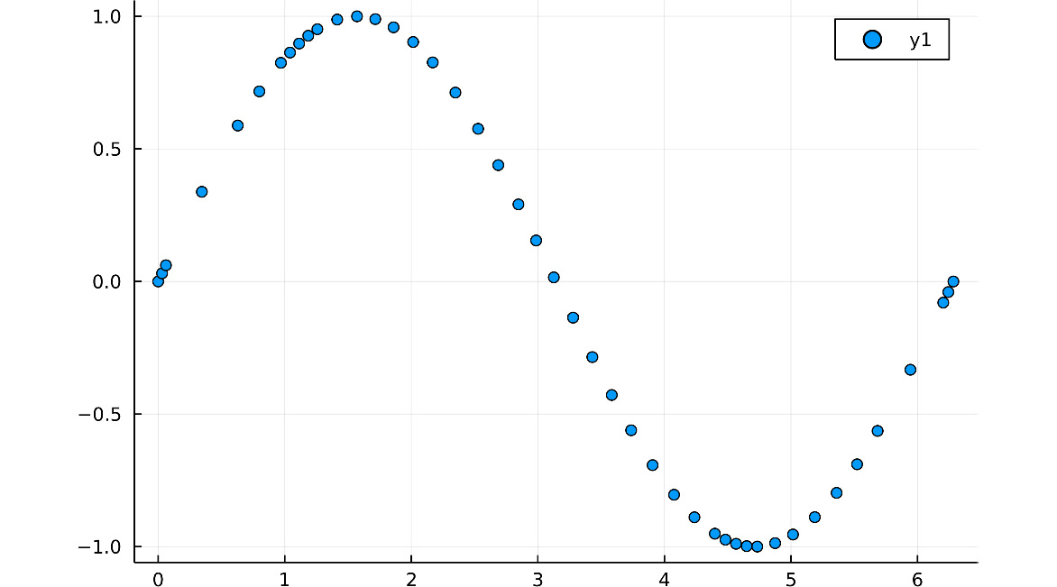
Figure 1.10 – A scatter plot

Note that the density of dots in the figure highlights the grid of x values that Plots created, using its adaptative algorithm to obtain a smooth line.

Bar plots

Bar plots are helpful when comparing a continuous variable, encoded as the bar height, across the different values of a discrete variable. We can construct them using the :bar series type or the bar and bar! functions. Another way to input data can come in handy when constructing bar plots – when we call the plot function using a single vector, range, or matrix as the first argument, Plots sets x to match the index number. Let's create a bar plot using this trick:

1. Run the following code:

   using Random
   heights = rand(MersenneTwister(1234), 10)

This creates a vector of random numbers to define the bar heights. We loaded the Random standard library to make a random number generator, with 1234 as a seed to see the same plot.

2. Execute bar(heights) to create a bar plot, where the first value of heights corresponds to x equal to one, the second is equal to two, and so on. Note that the value of x indicates the midpoint of the bar. The resulting plots should look like this:

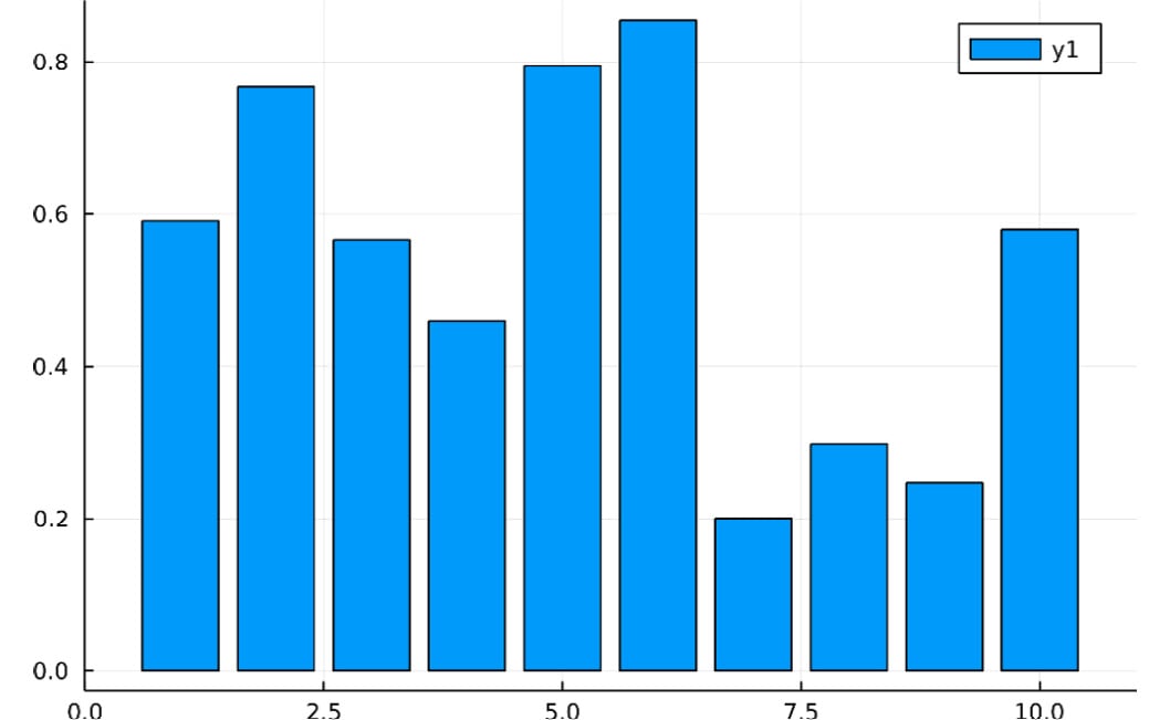
Figure 1.11 – A bar plot

You can also make x explicit by running bar(1:10, heights) on the last step; the result should be the same.

Heatmaps

The previous series type plotted a series for each column in an input matrix. Heatmaps are the plot type that we want if we prefer to see the structure of the input matrix. The magnitude of each value in the matrix is encoded using a color scale. Let's create a heatmap that matches the input matrix:

1. Execute the following code to create a 10 x 10 matrix:

   using Random
   matrix = rand(MersenneTwister(1), 10, 10)

2. Run hm = heatmap(matrix) to generate a heatmap. Note that the heatmap function plots the first matrix element at the bottom at (1, 1).
3. Execute plot!(hm, yflip=true) to fix that. Here, the plot! function modifies the value of the yflip attribute. yflip puts the value 1 of the y axis at the top when you set it to true. Now, the order colors match the order of the elements in the matrix:

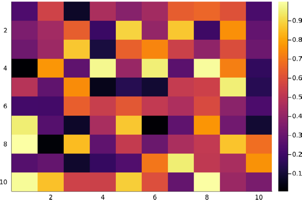
Figure 1.12 – A heatmap

We have seen how to create the most basic plot types using Plots. Let's now see how to compose them into single figures, taking advantage of the Plots layout system.

Simple layouts

Let's see the easiest way to compose multiple plots into a single figure. You can do it by simply passing plot objects to the plot function. By default, Plots will create a figure with a simple layout, where all plots have the same size. Plots orders the subplots according to their order in the attributes – for example, the following code creates a plot pane with two columns; the first column contains the plot of the sin function, and the second column the cos function plot:

plot(plot(cos), plot(sin))

In the following figure, we can see the plot created by the previous code:

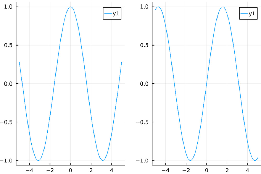
Figure 1.13 – A default subplot grid

We can use the grid function and the layout attribute of the plot function to customize the behavior – for example, we can have the two plots in a column rather than in a row by defining a grid with two rows and one column:

plot(plot(cos), plot(sin), layout = grid(2, 1))

The resulting plot will look like the one in the following figure:

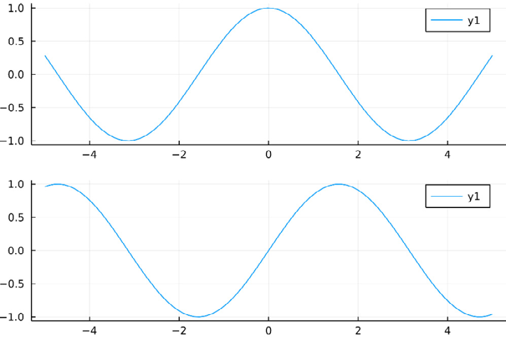
Figure 1.14 – A single-column layout

The grid function can take the widths and heights keyword arguments. Those arguments take a vector or tuple of floating-point numbers between 0 and 1, defining the relative proportion of the total width or height assigned to each subplot. Note that the length of the collection for widths should be identical to the number of columns, while the length for heights should match the number of rows in the grid layout – for example, the following code creates a panel with four plots arranged in a matrix of 2 by 2. The first column takes 80% (0.8) of the plot width, and the first row takes only 20% (0.2) of the total plot height:

plot(

    plot(sin), plot(cos),

    plot(asin), plot(acos),

    layout = grid(2, 2,

           heights=[0.2, 0.8],

           widths=[0.8, 0.2]),

    link = :x

    )

This code generates the following plots:

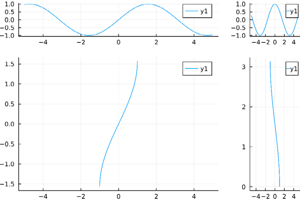
Figure 1.15 – A layout with user-defined sizes and linked x axes

Note that we have used the link attribute of a plot to link the x axes of each subplot column. You can use the link attribute to link the :x axes, the :y axes, or :both.

In those examples, we called the plot function inside the outer plot to create each argument, as each subplot is simple. It is better to store each subplot into variables for more complex figures. We will explore layouts in more depth in Chapter 11, Defining Plot Layouts to Create Figure Panels.

In this chapter, we have learned how to use Julia using different development environments, which will come in handy when developing interactive visualizations. We also learned how to install Julia packages, allowing us to access the Julia ecosystem's power. We also managed project environments to ensure the reproducibility of our projects through time and across computers. We have seen the most basic types and operations that you will need when creating plots in Julia. Finally, we have learned how to make some basic plots using the Plots package.

In the next chapter, we will learn more about the Julia ecosystem for data visualization. In particular, we will be going more into more depth about the Plots package to learn about its backends, and we will also explore Makie.

Here, we have only scratched the surface of the Julia language. If you want to learn more about it, its documentation is the best resource: https://docs.julialang.org/en/v1/.