This chapter will begin by identifying the target audience of this book, and will then go on to discuss the basic concepts and knowledge needed to use SQL query in SAP Business One. In the first section, you will be given a clear definition of the specific scope of the SQL and Query used in this book. The following section discusses the Data Dictionary and table links such as base tables versus target tables. The last section gives you a key concept to remember for building a good query by keeping it simple.
It may not be easy to deduce the ideal reader of this book. In fact, there are many different groups of SAP Business One users who may need this tool.
To my knowledge, there is no standard organization chart for Small and Midsized enterprises. Most of them are different. You may often find one person that handles more than one role. In this sense all users, especially end users, may need this book as long as they can use SQL query with the basic knowledge required.
You may check the following list to see if anything applies to you:
- Do you need to check specific sales results over certain time periods, for certain areas or certain customers?
- Do you want to know who the top vendors from certain locations for certain materials are?
- Do you have dynamic updated version of your sales force performance in real time?
- Do you often check if approval procedures are exactly matching your expectations?
- Have you tried to start building your SQL query but could not get it done properly?
- Have you experienced writing SQL query but the results are not always correct or up to your expectations?
If the answer to any of the questions mentioned earlier is "yes", then you can certainly benefit from reading this book. It will answer each and every question mentioned earlier and give you the power to solve complicated problems.
If you are an SAP Business One consultant, you have probably mastered SQL query already. However, if that is not the case, this book would be a great help to extend your consulting power. It will probably become a mandatory skill in the future that any SAP Business One consultant should be able to use SQL query.
If you are an SAP Business One add-on developer, these skills will be good additions to your capabilities. You may find this book useful even in some other development work like coding or programming. Very often you need to embed SQL query to your codes to complete your Software Development Kit (SDK) project.
If you are simply a normal SAP Business One end user, you may need this book more. This is because SQL query usage is best applied for the companies who have SAP Business One live data. Only you as the end users know better than anyone else what you are looking for to make Business Intelligence a daily routine job. It is very important for you to have an ability to create a query report so that you can map your requirement by query in a timely manner.
To the other readers who are not SAP Business One users, you could still get some hints and tips from this book because the working and the problematic queries are both shown. Even without an SAP Business One user interface, you may still gain some useful concepts. In one query example of this book, I will show you that even without the actual data from my database to test the query due to localization limitation, the correct answer to the questioner can still be deduced.
No matter what your background is, you will find this book useful whenever you need to get certain data quickly and accurately.
Before going into the details of SQL query, I would like to briefly introduce some basic database concepts because SQL is a database language for managing data in Relational Database Management Systems (RDBMS).
RDBMS is a Database Management System that is based on the relation model. Relational here is a key word for RDBMS. You will find that data is stored in the form of Tables and the relationship among the data is also stored in the form of tables for RDBMS.
Table is a key component within a database. One table or a group of tables represent one kind of data. For example, table OSLP within SAP Business One holds all Sales Employee Data. Tables are two-dimensional data storage place holders. You need to be familiar with their usage and their relationships with each other. If you are familiar with Microsoft Excel, the worksheet in Excel is a kind of two-dimensional table.
Table is also one of the most often used concepts in the book. Relationships between each table may be more important than tables themselves because without relation, nothing could be of any value. One important function within SAP Business One is allowing User Defined Table (UDT). All UDTs start with "@".

A field is the lowest unit holding data within a table. A table can have many fields. It is also called a column. Field and column are interchangeable. A table is comprised of records, and all records have the same structure with specific fields. One important concept in SAP Business One is User Defined Field (UDF). All UDFs start with U_.
SQL is often referred to as Structured Query Language. It is pronounced as S-Q-L or as the word "Sequel". There are many different revisions and extensions of SQL. The current revision is SQL: 2008, and the first major revision is SQL-92. Most of SQL extensions are built on top of SQL-92.
This book has very specific scope for the terms "SQL" and "query". Please read through this section carefully first if you find that the scope of the book is not right for your needs.
We have to limit the scope of the term SQL in this book. First of all, since SAP Business One is built on Microsoft SQL Server database, SQL here means Transact-SQL or T-SQL in brief. It is a Microsoft's/Sybase's extension of general meaning for SQL. Because we only use T-SQL throughout the book, SQL in this book will mean T-SQL unless it is clearly mentioned otherwise.
There are three main subsets of the SQL language:
Each set of the SQL language has a special purpose:
- DCL is used to control access to data in a database such as to grant or revoke specified users' rights to perform specified tasks.
- DDL is used to define data structures such as to create, alter, or drop tables.
- DML is used to retrieve and manipulate data in the table such as to insert, delete, and update data. Select, however, becomes a special statement belonging to this subset even though it is a read-only command that will not manipulate data at all.
Query is the most common operation in SQL. It could refer to all three SQL subsets. In this book, however, you will only learn the read-only part of the query. No Add, Delete, or Update SQL statement in DML will be discussed in the book since it is prohibited from SAP support policy for SAP Business One database integrity. All DCL or DDL SQL will also not be included because we neither control access to data in a database, nor define data structure for a database. You will find SELECT leading query only within the book. Read-only query SELECT has powerful functionality for finding useful information to meet your specific needs.
RDBMS
RDBMS is a Database Management System that is based on the relation model. Relational here is a key word for RDBMS. You will find that data is stored in the form of Tables and the relationship among the data is also stored in the form of tables for RDBMS.
Table is a key component within a database. One table or a group of tables represent one kind of data. For example, table OSLP within SAP Business One holds all Sales Employee Data. Tables are two-dimensional data storage place holders. You need to be familiar with their usage and their relationships with each other. If you are familiar with Microsoft Excel, the worksheet in Excel is a kind of two-dimensional table.
Table is also one of the most often used concepts in the book. Relationships between each table may be more important than tables themselves because without relation, nothing could be of any value. One important function within SAP Business One is allowing User Defined Table (UDT). All UDTs start with "@".
A field is the lowest unit holding data within a table. A table can have many fields. It is also called a column. Field and column are interchangeable. A table is comprised of records, and all records have the same structure with specific fields. One important concept in SAP Business One is User Defined Field (UDF). All UDFs start with U_.
SQL is often referred to as Structured Query Language. It is pronounced as S-Q-L or as the word "Sequel". There are many different revisions and extensions of SQL. The current revision is SQL: 2008, and the first major revision is SQL-92. Most of SQL extensions are built on top of SQL-92.
This book has very specific scope for the terms "SQL" and "query". Please read through this section carefully first if you find that the scope of the book is not right for your needs.
We have to limit the scope of the term SQL in this book. First of all, since SAP Business One is built on Microsoft SQL Server database, SQL here means Transact-SQL or T-SQL in brief. It is a Microsoft's/Sybase's extension of general meaning for SQL. Because we only use T-SQL throughout the book, SQL in this book will mean T-SQL unless it is clearly mentioned otherwise.
There are three main subsets of the SQL language:
Each set of the SQL language has a special purpose:
- DCL is used to control access to data in a database such as to grant or revoke specified users' rights to perform specified tasks.
- DDL is used to define data structures such as to create, alter, or drop tables.
- DML is used to retrieve and manipulate data in the table such as to insert, delete, and update data. Select, however, becomes a special statement belonging to this subset even though it is a read-only command that will not manipulate data at all.
Query is the most common operation in SQL. It could refer to all three SQL subsets. In this book, however, you will only learn the read-only part of the query. No Add, Delete, or Update SQL statement in DML will be discussed in the book since it is prohibited from SAP support policy for SAP Business One database integrity. All DCL or DDL SQL will also not be included because we neither control access to data in a database, nor define data structure for a database. You will find SELECT leading query only within the book. Read-only query SELECT has powerful functionality for finding useful information to meet your specific needs.
Table
Table is a key component within a database. One table or a group of tables represent one kind of data. For example, table OSLP within SAP Business One holds all Sales Employee Data. Tables are two-dimensional data storage place holders. You need to be familiar with their usage and their relationships with each other. If you are familiar with Microsoft Excel, the worksheet in Excel is a kind of two-dimensional table.
Table is also one of the most often used concepts in the book. Relationships between each table may be more important than tables themselves because without relation, nothing could be of any value. One important function within SAP Business One is allowing User Defined Table (UDT). All UDTs start with "@".
A field is the lowest unit holding data within a table. A table can have many fields. It is also called a column. Field and column are interchangeable. A table is comprised of records, and all records have the same structure with specific fields. One important concept in SAP Business One is User Defined Field (UDF). All UDFs start with U_.
SQL is often referred to as Structured Query Language. It is pronounced as S-Q-L or as the word "Sequel". There are many different revisions and extensions of SQL. The current revision is SQL: 2008, and the first major revision is SQL-92. Most of SQL extensions are built on top of SQL-92.
This book has very specific scope for the terms "SQL" and "query". Please read through this section carefully first if you find that the scope of the book is not right for your needs.
We have to limit the scope of the term SQL in this book. First of all, since SAP Business One is built on Microsoft SQL Server database, SQL here means Transact-SQL or T-SQL in brief. It is a Microsoft's/Sybase's extension of general meaning for SQL. Because we only use T-SQL throughout the book, SQL in this book will mean T-SQL unless it is clearly mentioned otherwise.
There are three main subsets of the SQL language:
Each set of the SQL language has a special purpose:
- DCL is used to control access to data in a database such as to grant or revoke specified users' rights to perform specified tasks.
- DDL is used to define data structures such as to create, alter, or drop tables.
- DML is used to retrieve and manipulate data in the table such as to insert, delete, and update data. Select, however, becomes a special statement belonging to this subset even though it is a read-only command that will not manipulate data at all.
Query is the most common operation in SQL. It could refer to all three SQL subsets. In this book, however, you will only learn the read-only part of the query. No Add, Delete, or Update SQL statement in DML will be discussed in the book since it is prohibited from SAP support policy for SAP Business One database integrity. All DCL or DDL SQL will also not be included because we neither control access to data in a database, nor define data structure for a database. You will find SELECT leading query only within the book. Read-only query SELECT has powerful functionality for finding useful information to meet your specific needs.
Field
A field is the lowest unit holding data within a table. A table can have many fields. It is also called a column. Field and column are interchangeable. A table is comprised of records, and all records have the same structure with specific fields. One important concept in SAP Business One is User Defined Field (UDF). All UDFs start with U_.
SQL is often referred to as Structured Query Language. It is pronounced as S-Q-L or as the word "Sequel". There are many different revisions and extensions of SQL. The current revision is SQL: 2008, and the first major revision is SQL-92. Most of SQL extensions are built on top of SQL-92.
This book has very specific scope for the terms "SQL" and "query". Please read through this section carefully first if you find that the scope of the book is not right for your needs.
We have to limit the scope of the term SQL in this book. First of all, since SAP Business One is built on Microsoft SQL Server database, SQL here means Transact-SQL or T-SQL in brief. It is a Microsoft's/Sybase's extension of general meaning for SQL. Because we only use T-SQL throughout the book, SQL in this book will mean T-SQL unless it is clearly mentioned otherwise.
There are three main subsets of the SQL language:
Each set of the SQL language has a special purpose:
- DCL is used to control access to data in a database such as to grant or revoke specified users' rights to perform specified tasks.
- DDL is used to define data structures such as to create, alter, or drop tables.
- DML is used to retrieve and manipulate data in the table such as to insert, delete, and update data. Select, however, becomes a special statement belonging to this subset even though it is a read-only command that will not manipulate data at all.
Query is the most common operation in SQL. It could refer to all three SQL subsets. In this book, however, you will only learn the read-only part of the query. No Add, Delete, or Update SQL statement in DML will be discussed in the book since it is prohibited from SAP support policy for SAP Business One database integrity. All DCL or DDL SQL will also not be included because we neither control access to data in a database, nor define data structure for a database. You will find SELECT leading query only within the book. Read-only query SELECT has powerful functionality for finding useful information to meet your specific needs.
SQL
SQL is often referred to as Structured Query Language. It is pronounced as S-Q-L or as the word "Sequel". There are many different revisions and extensions of SQL. The current revision is SQL: 2008, and the first major revision is SQL-92. Most of SQL extensions are built on top of SQL-92.
This book has very specific scope for the terms "SQL" and "query". Please read through this section carefully first if you find that the scope of the book is not right for your needs.
We have to limit the scope of the term SQL in this book. First of all, since SAP Business One is built on Microsoft SQL Server database, SQL here means Transact-SQL or T-SQL in brief. It is a Microsoft's/Sybase's extension of general meaning for SQL. Because we only use T-SQL throughout the book, SQL in this book will mean T-SQL unless it is clearly mentioned otherwise.
There are three main subsets of the SQL language:
Each set of the SQL language has a special purpose:
- DCL is used to control access to data in a database such as to grant or revoke specified users' rights to perform specified tasks.
- DDL is used to define data structures such as to create, alter, or drop tables.
- DML is used to retrieve and manipulate data in the table such as to insert, delete, and update data. Select, however, becomes a special statement belonging to this subset even though it is a read-only command that will not manipulate data at all.
Query is the most common operation in SQL. It could refer to all three SQL subsets. In this book, however, you will only learn the read-only part of the query. No Add, Delete, or Update SQL statement in DML will be discussed in the book since it is prohibited from SAP support policy for SAP Business One database integrity. All DCL or DDL SQL will also not be included because we neither control access to data in a database, nor define data structure for a database. You will find SELECT leading query only within the book. Read-only query SELECT has powerful functionality for finding useful information to meet your specific needs.
T-SQL
We have to limit the scope of the term SQL in this book. First of all, since SAP Business One is built on Microsoft SQL Server database, SQL here means Transact-SQL or T-SQL in brief. It is a Microsoft's/Sybase's extension of general meaning for SQL. Because we only use T-SQL throughout the book, SQL in this book will mean T-SQL unless it is clearly mentioned otherwise.
There are three main subsets of the SQL language:
Each set of the SQL language has a special purpose:
- DCL is used to control access to data in a database such as to grant or revoke specified users' rights to perform specified tasks.
- DDL is used to define data structures such as to create, alter, or drop tables.
- DML is used to retrieve and manipulate data in the table such as to insert, delete, and update data. Select, however, becomes a special statement belonging to this subset even though it is a read-only command that will not manipulate data at all.
Query is the most common operation in SQL. It could refer to all three SQL subsets. In this book, however, you will only learn the read-only part of the query. No Add, Delete, or Update SQL statement in DML will be discussed in the book since it is prohibited from SAP support policy for SAP Business One database integrity. All DCL or DDL SQL will also not be included because we neither control access to data in a database, nor define data structure for a database. You will find SELECT leading query only within the book. Read-only query SELECT has powerful functionality for finding useful information to meet your specific needs.
Subsets of SQL
There are three main subsets of the SQL language:
Each set of the SQL language has a special purpose:
- DCL is used to control access to data in a database such as to grant or revoke specified users' rights to perform specified tasks.
- DDL is used to define data structures such as to create, alter, or drop tables.
- DML is used to retrieve and manipulate data in the table such as to insert, delete, and update data. Select, however, becomes a special statement belonging to this subset even though it is a read-only command that will not manipulate data at all.
Query is the most common operation in SQL. It could refer to all three SQL subsets. In this book, however, you will only learn the read-only part of the query. No Add, Delete, or Update SQL statement in DML will be discussed in the book since it is prohibited from SAP support policy for SAP Business One database integrity. All DCL or DDL SQL will also not be included because we neither control access to data in a database, nor define data structure for a database. You will find SELECT leading query only within the book. Read-only query SELECT has powerful functionality for finding useful information to meet your specific needs.
Query
Query is the most common operation in SQL. It could refer to all three SQL subsets. In this book, however, you will only learn the read-only part of the query. No Add, Delete, or Update SQL statement in DML will be discussed in the book since it is prohibited from SAP support policy for SAP Business One database integrity. All DCL or DDL SQL will also not be included because we neither control access to data in a database, nor define data structure for a database. You will find SELECT leading query only within the book. Read-only query SELECT has powerful functionality for finding useful information to meet your specific needs.
In order to create working SQL queries, you not only need to know how to write it, but also need to have a clear view regarding the relationship between tables and where to find the information required. As you know, SAP Business One is built on Microsoft SQL Server. Data dictionary is a great tool for creating SQL queries. Before we start, a good Data Dictionary is essential for the database. Fortunately, there is a very good reference called SAP Business One Database Tables Reference readily available through SAP Business One SDK help Centre. You can find the details in the following section.
The database tables reference file named REFDB.CHM is the one we are looking for. SDK is usually installed on the same server as the SAP Business One database server. Normally, the file path is: X:\Program Files\SAP\SAP Business One SDK\Help. Here, "X" means the drive where your SAP Business One SDK is installed. The help file looks like this:
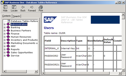
In this help file, we will find the same categories as the SAP Business One menu with all 11 modules. The tables related to each module are listed one by one. There are tree structures in the help file if the header tables have row tables. Each table provides a list of all the fields in the table along with their description, type, size, related tables, default value, and constraints.
To help you understand the previous mentioned data dictionary quickly, we will be going through the naming conventions for the table in SAP Business One.
Most tables for SAP Business One have four letters. The only exceptions are number-ending tables, if the numbers are greater than nine. Those tables will have five letters. To understand table names easily, there is a three letter abbreviation in SAP Business One. Some of the commonly used abbreviations are listed as follows:
- ADM: Administration
- ATC: Attachments
- CPR: Contact Persons
- CRD: Business Partners
- DLN: Delivery Notes
- HEM: Employees
- INV: Sales Invoices
- ITM: Items
- ITT: Product Trees (Bill of Materials)
- OPR: Sales Opportunities
- PCH: Purchase Invoices
- PDN: Goods Receipt PO
- POR: Purchase Orders
- QUT: Sales Quotations
- RDR: Sales Orders
- RIN: Sales Credit Notes
- RPC: Purchase Credit Notes
- SLP: Sales Employees
- USR: Users
- WOR: Production Orders
- WTR: Stock Transfers
All tables starting with "O" refer to master tables. O here represents Object. For example:
- OITM: Items Master
- OCRD: Business Partners Master
- OSLP: Sales Employee
Most tables starting with "A" may mean historical log tables. A here represents Archive. For example:
- AITM: Items—History
- ACRD: Business Partners—History
- AUSR: Archive Users—History
These are special O tables with the exact same structure. They can be tables related to Sales or Purchase. These are called Marketing Documents. These also include most Inventory transaction tables. Some examples are:
- OINV: A/R Invoice Header
- OPCH: A/P Invoice Header
- OIGN: Goods Receipt Header
All tables ending with a number refer to document line detail tables or subtables for the master table. Numbers here could refer to different properties of the header tables.
- INV1: A/R Invoice Row
- PCH1: A/P Invoice Row
- IGN1: Goods Receipt Row
- INV2: A/R Invoice—Row Expense
Some specific tables very important for query building are listed here:
- OJDT-Journal Entry: This table includes all financial journal entries no matter whether they are automatically posted or manually posted.
- OINM-Warehouse Journal: This table includes all inventory-related transactions. It is a single point to check everything in relation to your inventory (or stock). It becomes a view in the new version. This view must be queried very carefully.
- ADOC-Document History: This table includes all document history. However, it is wrongly named in the documentation, "Invoice History" table in the help file.
SAP Business One—Database tables reference
The database tables reference file named REFDB.CHM is the one we are looking for. SDK is usually installed on the same server as the SAP Business One database server. Normally, the file path is: X:\Program Files\SAP\SAP Business One SDK\Help. Here, "X" means the drive where your SAP Business One SDK is installed. The help file looks like this:
In this help file, we will find the same categories as the SAP Business One menu with all 11 modules. The tables related to each module are listed one by one. There are tree structures in the help file if the header tables have row tables. Each table provides a list of all the fields in the table along with their description, type, size, related tables, default value, and constraints.
To help you understand the previous mentioned data dictionary quickly, we will be going through the naming conventions for the table in SAP Business One.
Most tables for SAP Business One have four letters. The only exceptions are number-ending tables, if the numbers are greater than nine. Those tables will have five letters. To understand table names easily, there is a three letter abbreviation in SAP Business One. Some of the commonly used abbreviations are listed as follows:
- ADM: Administration
- ATC: Attachments
- CPR: Contact Persons
- CRD: Business Partners
- DLN: Delivery Notes
- HEM: Employees
- INV: Sales Invoices
- ITM: Items
- ITT: Product Trees (Bill of Materials)
- OPR: Sales Opportunities
- PCH: Purchase Invoices
- PDN: Goods Receipt PO
- POR: Purchase Orders
- QUT: Sales Quotations
- RDR: Sales Orders
- RIN: Sales Credit Notes
- RPC: Purchase Credit Notes
- SLP: Sales Employees
- USR: Users
- WOR: Production Orders
- WTR: Stock Transfers
All tables starting with "O" refer to master tables. O here represents Object. For example:
- OITM: Items Master
- OCRD: Business Partners Master
- OSLP: Sales Employee
Most tables starting with "A" may mean historical log tables. A here represents Archive. For example:
- AITM: Items—History
- ACRD: Business Partners—History
- AUSR: Archive Users—History
These are special O tables with the exact same structure. They can be tables related to Sales or Purchase. These are called Marketing Documents. These also include most Inventory transaction tables. Some examples are:
- OINV: A/R Invoice Header
- OPCH: A/P Invoice Header
- OIGN: Goods Receipt Header
All tables ending with a number refer to document line detail tables or subtables for the master table. Numbers here could refer to different properties of the header tables.
- INV1: A/R Invoice Row
- PCH1: A/P Invoice Row
- IGN1: Goods Receipt Row
- INV2: A/R Invoice—Row Expense
Some specific tables very important for query building are listed here:
- OJDT-Journal Entry: This table includes all financial journal entries no matter whether they are automatically posted or manually posted.
- OINM-Warehouse Journal: This table includes all inventory-related transactions. It is a single point to check everything in relation to your inventory (or stock). It becomes a view in the new version. This view must be queried very carefully.
- ADOC-Document History: This table includes all document history. However, it is wrongly named in the documentation, "Invoice History" table in the help file.
Naming convention of tables for SAP Business One
To help you understand the previous mentioned data dictionary quickly, we will be going through the naming conventions for the table in SAP Business One.
Most tables for SAP Business One have four letters. The only exceptions are number-ending tables, if the numbers are greater than nine. Those tables will have five letters. To understand table names easily, there is a three letter abbreviation in SAP Business One. Some of the commonly used abbreviations are listed as follows:
- ADM: Administration
- ATC: Attachments
- CPR: Contact Persons
- CRD: Business Partners
- DLN: Delivery Notes
- HEM: Employees
- INV: Sales Invoices
- ITM: Items
- ITT: Product Trees (Bill of Materials)
- OPR: Sales Opportunities
- PCH: Purchase Invoices
- PDN: Goods Receipt PO
- POR: Purchase Orders
- QUT: Sales Quotations
- RDR: Sales Orders
- RIN: Sales Credit Notes
- RPC: Purchase Credit Notes
- SLP: Sales Employees
- USR: Users
- WOR: Production Orders
- WTR: Stock Transfers
All tables starting with "O" refer to master tables. O here represents Object. For example:
- OITM: Items Master
- OCRD: Business Partners Master
- OSLP: Sales Employee
Most tables starting with "A" may mean historical log tables. A here represents Archive. For example:
- AITM: Items—History
- ACRD: Business Partners—History
- AUSR: Archive Users—History
These are special O tables with the exact same structure. They can be tables related to Sales or Purchase. These are called Marketing Documents. These also include most Inventory transaction tables. Some examples are:
- OINV: A/R Invoice Header
- OPCH: A/P Invoice Header
- OIGN: Goods Receipt Header
All tables ending with a number refer to document line detail tables or subtables for the master table. Numbers here could refer to different properties of the header tables.
- INV1: A/R Invoice Row
- PCH1: A/P Invoice Row
- IGN1: Goods Receipt Row
- INV2: A/R Invoice—Row Expense
Some specific tables very important for query building are listed here:
- OJDT-Journal Entry: This table includes all financial journal entries no matter whether they are automatically posted or manually posted.
- OINM-Warehouse Journal: This table includes all inventory-related transactions. It is a single point to check everything in relation to your inventory (or stock). It becomes a view in the new version. This view must be queried very carefully.
- ADOC-Document History: This table includes all document history. However, it is wrongly named in the documentation, "Invoice History" table in the help file.
Three letter words
Most tables for SAP Business One have four letters. The only exceptions are number-ending tables, if the numbers are greater than nine. Those tables will have five letters. To understand table names easily, there is a three letter abbreviation in SAP Business One. Some of the commonly used abbreviations are listed as follows:
- ADM: Administration
- ATC: Attachments
- CPR: Contact Persons
- CRD: Business Partners
- DLN: Delivery Notes
- HEM: Employees
- INV: Sales Invoices
- ITM: Items
- ITT: Product Trees (Bill of Materials)
- OPR: Sales Opportunities
- PCH: Purchase Invoices
- PDN: Goods Receipt PO
- POR: Purchase Orders
- QUT: Sales Quotations
- RDR: Sales Orders
- RIN: Sales Credit Notes
- RPC: Purchase Credit Notes
- SLP: Sales Employees
- USR: Users
- WOR: Production Orders
- WTR: Stock Transfers
All tables starting with "O" refer to master tables. O here represents Object. For example:
- OITM: Items Master
- OCRD: Business Partners Master
- OSLP: Sales Employee
Most tables starting with "A" may mean historical log tables. A here represents Archive. For example:
- AITM: Items—History
- ACRD: Business Partners—History
- AUSR: Archive Users—History
These are special O tables with the exact same structure. They can be tables related to Sales or Purchase. These are called Marketing Documents. These also include most Inventory transaction tables. Some examples are:
- OINV: A/R Invoice Header
- OPCH: A/P Invoice Header
- OIGN: Goods Receipt Header
All tables ending with a number refer to document line detail tables or subtables for the master table. Numbers here could refer to different properties of the header tables.
- INV1: A/R Invoice Row
- PCH1: A/P Invoice Row
- IGN1: Goods Receipt Row
- INV2: A/R Invoice—Row Expense
Some specific tables very important for query building are listed here:
- OJDT-Journal Entry: This table includes all financial journal entries no matter whether they are automatically posted or manually posted.
- OINM-Warehouse Journal: This table includes all inventory-related transactions. It is a single point to check everything in relation to your inventory (or stock). It becomes a view in the new version. This view must be queried very carefully.
- ADOC-Document History: This table includes all document history. However, it is wrongly named in the documentation, "Invoice History" table in the help file.
"O" tables
All tables starting with "O" refer to master tables. O here represents Object. For example:
- OITM: Items Master
- OCRD: Business Partners Master
- OSLP: Sales Employee
Most tables starting with "A" may mean historical log tables. A here represents Archive. For example:
- AITM: Items—History
- ACRD: Business Partners—History
- AUSR: Archive Users—History
These are special O tables with the exact same structure. They can be tables related to Sales or Purchase. These are called Marketing Documents. These also include most Inventory transaction tables. Some examples are:
- OINV: A/R Invoice Header
- OPCH: A/P Invoice Header
- OIGN: Goods Receipt Header
All tables ending with a number refer to document line detail tables or subtables for the master table. Numbers here could refer to different properties of the header tables.
- INV1: A/R Invoice Row
- PCH1: A/P Invoice Row
- IGN1: Goods Receipt Row
- INV2: A/R Invoice—Row Expense
Some specific tables very important for query building are listed here:
- OJDT-Journal Entry: This table includes all financial journal entries no matter whether they are automatically posted or manually posted.
- OINM-Warehouse Journal: This table includes all inventory-related transactions. It is a single point to check everything in relation to your inventory (or stock). It becomes a view in the new version. This view must be queried very carefully.
- ADOC-Document History: This table includes all document history. However, it is wrongly named in the documentation, "Invoice History" table in the help file.
"A" tables
Most tables starting with "A" may mean historical log tables. A here represents Archive. For example:
- AITM: Items—History
- ACRD: Business Partners—History
- AUSR: Archive Users—History
These are special O tables with the exact same structure. They can be tables related to Sales or Purchase. These are called Marketing Documents. These also include most Inventory transaction tables. Some examples are:
- OINV: A/R Invoice Header
- OPCH: A/P Invoice Header
- OIGN: Goods Receipt Header
All tables ending with a number refer to document line detail tables or subtables for the master table. Numbers here could refer to different properties of the header tables.
- INV1: A/R Invoice Row
- PCH1: A/P Invoice Row
- IGN1: Goods Receipt Row
- INV2: A/R Invoice—Row Expense
Some specific tables very important for query building are listed here:
- OJDT-Journal Entry: This table includes all financial journal entries no matter whether they are automatically posted or manually posted.
- OINM-Warehouse Journal: This table includes all inventory-related transactions. It is a single point to check everything in relation to your inventory (or stock). It becomes a view in the new version. This view must be queried very carefully.
- ADOC-Document History: This table includes all document history. However, it is wrongly named in the documentation, "Invoice History" table in the help file.
Document header tables
These are special O tables with the exact same structure. They can be tables related to Sales or Purchase. These are called Marketing Documents. These also include most Inventory transaction tables. Some examples are:
- OINV: A/R Invoice Header
- OPCH: A/P Invoice Header
- OIGN: Goods Receipt Header
All tables ending with a number refer to document line detail tables or subtables for the master table. Numbers here could refer to different properties of the header tables.
- INV1: A/R Invoice Row
- PCH1: A/P Invoice Row
- IGN1: Goods Receipt Row
- INV2: A/R Invoice—Row Expense
Some specific tables very important for query building are listed here:
- OJDT-Journal Entry: This table includes all financial journal entries no matter whether they are automatically posted or manually posted.
- OINM-Warehouse Journal: This table includes all inventory-related transactions. It is a single point to check everything in relation to your inventory (or stock). It becomes a view in the new version. This view must be queried very carefully.
- ADOC-Document History: This table includes all document history. However, it is wrongly named in the documentation, "Invoice History" table in the help file.
Document line tables
All tables ending with a number refer to document line detail tables or subtables for the master table. Numbers here could refer to different properties of the header tables.
- INV1: A/R Invoice Row
- PCH1: A/P Invoice Row
- IGN1: Goods Receipt Row
- INV2: A/R Invoice—Row Expense
Some specific tables very important for query building are listed here:
- OJDT-Journal Entry: This table includes all financial journal entries no matter whether they are automatically posted or manually posted.
- OINM-Warehouse Journal: This table includes all inventory-related transactions. It is a single point to check everything in relation to your inventory (or stock). It becomes a view in the new version. This view must be queried very carefully.
- ADOC-Document History: This table includes all document history. However, it is wrongly named in the documentation, "Invoice History" table in the help file.
Important table examples
Some specific tables very important for query building are listed here:
- OJDT-Journal Entry: This table includes all financial journal entries no matter whether they are automatically posted or manually posted.
- OINM-Warehouse Journal: This table includes all inventory-related transactions. It is a single point to check everything in relation to your inventory (or stock). It becomes a view in the new version. This view must be queried very carefully.
- ADOC-Document History: This table includes all document history. However, it is wrongly named in the documentation, "Invoice History" table in the help file.
Table links are fundamental for query building. You will see some different links in this section, but the most common links will be discussed in the next section because there are too many and they are used too often.
To understand table links, you need to know more about table structures.
Every table has a primary key. Some of the tables have foreign keys too. All those keys are used for the index. Docentry is a typical primary key to link OXXX with XXXn document tables. For example, Docentry is a common key field to link OPOR with POR1, POR2 to POR12.
A primary key can be one or more fields. For a simple table one key field would be good enough. For a complicated table, two or more fields for primary key are not rare.
A primary key has to be unique within the same table. This key will not allow NULL value—that is, an empty field or a field with no data.
A foreign key is usually used to link to some other table's primary key. This field will be updated whenever the other table record has changed.
Although, you could link any fields between tables, if the field is not NULL, you should try to use key link wherever possible in order to increase the database performance.
To be clearer about the link, here are a few table link examples:
- OITM-Items table and ITM1-Items Prices table:
These two tables are linked through ItemCode field. Both tables have the same field name to link. It is not one-to-one but one-to-many relationships. One Item Code in item master may have more than one item price associated.
- OITT-Product Tree table and ITT1-Product Tree Child Items:
These two tables are linked through Code field in OITT and Father field in ITT1. These tables are used for Bill of Materials.
- OCRD-Business Partner table and OSLP-Sales Employee table:
These two tables are linked through the same name field SlpCode. In the second table, SlpCode is the primary key for OSLP. On the other hand, it is a foreign key in the first table OCRD.
Primary key
Every table has a primary key. Some of the tables have foreign keys too. All those keys are used for the index. Docentry is a typical primary key to link OXXX with XXXn document tables. For example, Docentry is a common key field to link OPOR with POR1, POR2 to POR12.
A primary key can be one or more fields. For a simple table one key field would be good enough. For a complicated table, two or more fields for primary key are not rare.
A primary key has to be unique within the same table. This key will not allow NULL value—that is, an empty field or a field with no data.
A foreign key is usually used to link to some other table's primary key. This field will be updated whenever the other table record has changed.
Although, you could link any fields between tables, if the field is not NULL, you should try to use key link wherever possible in order to increase the database performance.
To be clearer about the link, here are a few table link examples:
- OITM-Items table and ITM1-Items Prices table:
These two tables are linked through ItemCode field. Both tables have the same field name to link. It is not one-to-one but one-to-many relationships. One Item Code in item master may have more than one item price associated.
- OITT-Product Tree table and ITT1-Product Tree Child Items:
These two tables are linked through Code field in OITT and Father field in ITT1. These tables are used for Bill of Materials.
- OCRD-Business Partner table and OSLP-Sales Employee table:
These two tables are linked through the same name field SlpCode. In the second table, SlpCode is the primary key for OSLP. On the other hand, it is a foreign key in the first table OCRD.
Foreign key
A foreign key is usually used to link to some other table's primary key. This field will be updated whenever the other table record has changed.
Although, you could link any fields between tables, if the field is not NULL, you should try to use key link wherever possible in order to increase the database performance.
To be clearer about the link, here are a few table link examples:
- OITM-Items table and ITM1-Items Prices table:
These two tables are linked through ItemCode field. Both tables have the same field name to link. It is not one-to-one but one-to-many relationships. One Item Code in item master may have more than one item price associated.
- OITT-Product Tree table and ITT1-Product Tree Child Items:
These two tables are linked through Code field in OITT and Father field in ITT1. These tables are used for Bill of Materials.
- OCRD-Business Partner table and OSLP-Sales Employee table:
These two tables are linked through the same name field SlpCode. In the second table, SlpCode is the primary key for OSLP. On the other hand, it is a foreign key in the first table OCRD.
Example of table links within SAP Business One
To be clearer about the link, here are a few table link examples:
- OITM-Items table and ITM1-Items Prices table:
These two tables are linked through ItemCode field. Both tables have the same field name to link. It is not one-to-one but one-to-many relationships. One Item Code in item master may have more than one item price associated.
- OITT-Product Tree table and ITT1-Product Tree Child Items:
These two tables are linked through Code field in OITT and Father field in ITT1. These tables are used for Bill of Materials.
- OCRD-Business Partner table and OSLP-Sales Employee table:
These two tables are linked through the same name field SlpCode. In the second table, SlpCode is the primary key for OSLP. On the other hand, it is a foreign key in the first table OCRD.
Base tables and target tables are special linked tables within SAP Business One. They are the most often used linked tables for SQL queries too.
You may find most of them related to "Sales-A/R" and "Purchase-A/P" documents or so-called "Marketing Documents".
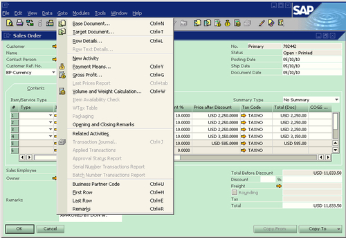
Marketing documents may not have base tables or target tables. From the previous screenshot, you could clearly find that the Base Document and Target Document are available to this Sales Order. To get the Base Document, you may click on the "left arrow icon" or use the shortcut key Ctrl+N. To get the Target Document, you may click on the "right arrow icon" or use the shortcut key Ctrl+T. Only when the base table or target table is available to the current document, will you find the menu items and icons in active status. Otherwise, both icons and menu items are grayed out.
From the terms "Base" and "Target", it is clear that the target table can be based upon the base table.
One table could be based on different types of tables:

From this demonstration, you could get a clear picture about the relationship between Base Document (table) and Target Document (table). A specific pair of Purchase Order and Good Receipt PO tables is shown here. This concept applies to all document type tables. Here is a list of commonly used base-target pairs; they are not inclusive. You may find more, but the following are the most frequently used ones:
|
Base Table |
Target Table |
|---|---|
|
OQUT—Sales Quotation |
ORDR—Sales Order |
|
OQUT—Sales Quotation |
ODLN—Delivery |
|
OQUT—Sales Quotation |
OINV—A/R Invoice |
|
ORDR—Sales Order |
ODLN—Delivery |
|
ORDR—Sales Order |
OINV—A/R Invoice |
|
ODLN—Delivery |
ORDN—Returns |
|
ODLN—Delivery |
OINV—A/R Invoice |
|
ORDN—Returns |
ORIN—A/R Credit Note |
|
ODLN—A/R Invoice |
ORIN—A/R Credit Note |
|
OPOR—Purchase Order |
OPDN—Goods Receipt PO |
|
OPOR—Purchase Order |
OPCH—A/P Invoice |
|
OPDN—Goods Receipt PO |
ORPD—Goods return |
|
OPDN—Goods Receipt PO |
OPCH—A/P Invoice |
|
ORPD—Goods return |
ORPC—A/P Credit Note |
|
OPCH—A/P Invoice |
ORPC—A/P Credit Note |
I have omitted the details for the link. Actually, you will find that all the links exist on the first child table or so-called row table for the header table, such as QUT1 instead of OQUT.
The linking fields are very clear. For example:
- BaseEntry in the target table refers to the base table's DocEntry
- BaseType refers to the types of the base table
- BaseRef is usually linked to DocNum field in the base table
- BaseLine will be the line number in the base line table
- TargetEntry in the base table refers to the target table's DocEntry
- TargetType refers to the types of the target table
Before you go on to the next chapter, an important concept needs to be kept in mind:
Simplicity is in need everywhere in the current changing world. Wherever you make things complicated, you may find yourself in an awkward position to compete with others.
My slogan is: simple, simpler, the simplest.
I have a habit in query building: the last step for any new query would be checking to see if it is the simplest one. In this way, "keep it simple" would not only be kept in the already built query, but also helps new queries to be the simplest in the beginning.
By keeping a query as simple as possible, it will ensure that the system performance is not affected. It will also be a great help to the troubleshooting process. A short checklist for simplicity is as follows:
- Other queries: Are there any other queries doing a similar job, and if yes, why does the new query need to be built?
- Tables: Are there any tables that have not been used for the query?
- Fields: Are there any fields that have not been used for the query?
- Conditions: Are there any condition overlaps?
The list can be much longer. The meaning behind it is clear: there is a never ending battle to get rid of complications.
When you try this method and it becomes a routine, you will find that query building becomes an enjoyable process.
In this chapter, you have been identified to be an appropriate reader who needs this information, supposing that you read through the beginning chapter and still want to read more.
You have been given all the basic concepts such as RDBMS, Table, SQL, T-SQL, SQL Subsets, and Query. You also get the idea of what the strict meanings of "SQL" and "Query" are within this book.
By going deeper into discussing table relationships, you gained a bigger picture of SAP Business One's database structure and tables' naming conventions. You also learned about base tables versus target tables in SAP Business One.
The "Keep it simple" principle has been emphasized in the last section of the chapter. You are advised to use it whenever you practice your own queries.
The next chapter will introduce you to the Query Generator and Query Wizard tools, so that you can start hands-on in building SQL query as soon as possible, if you have not yet done so.
In the previous chapter, you learned basic concepts regarding certain terminologies used in this book. You also know that tables and table relationships are important for SQL Query. What are all of these concepts about? You will better understand when you start your own journey to create a SQL Query report.
How do I start? That is a good question. I have learned this the hard way. Even though the tools to create queries are readily available from the SAP Business One menu, I myself had never gone through most of these tools before I planned to write this book to show you how to start. I have kept using only Query Manager and system queries until now. To be honest, I just found out too late that I took such a longer route than necessary. What a pity! If I had started with Query Generator and Query Wizard, it would have saved me a tremendous amount of time.
These tools are quite convenient and efficient for everyone to use, especially for starters to write their first query for SAP Business One. These tools will help you to omit this process of writing every single statement, tables' names, or fields' names, etc.
This chapter will introduce you to two basic SQL Query tools for SAP Business One:
Both tools are for starters to get to know SQL query in SAP Business One quickly. After you have learned these tools, you could get a simple job done just with a few mouse clicks. The introduction gives you detailed steps so that you can have step-by-step advice.
In the next section, the differences between these tools are discussed. You can decide which one is more suitable for you when you read through all their features and benefits.
If you are a more experienced reader, you may find that these tools are no longer necessary. Otherwise, you are strongly encouraged to go through the chapter to refresh yourself.
The last section introduces System Queries built-in to SAP Business One. Those system queries are another good start for readers whose SQL Query level is above average. You could then customize them and create your own queries quickly. For a beginner, you may just learn how to run those queries first to save time.

The previous screenshot shows you how to access these different tools from the SAP Business One menu. You can find all tools for this chapter from it. They are all under the Tools | Queries menu. Query Generator is the second item; Query Wizard is the third item; and System Queries is number five.
Query Generator is the first tool to be discussed. It is located above the Query Wizard in the menu item list.
Query Generator enables you to create queries using the SQL query engine. Like all other tools, it is designed for data retrieval/selection only. You are not able to do any DML queries such as updates, insert, or delete. This menu item can be accessed from Tools | Queries | Query Generator.
With this tool, you are able to:
- Create many queries yourself from a fixed set of tables in SAP Business One
- Access all the data in those tables and evaluate it according to your needs
- Create individual reports without writing any single query statements
After you click on the Query Generator menu item, you can bring up the main form of Query Generator. On the top left of the form, you may find a yellow cell. Click the Tab key from the empty cell to bring up Choose from List, as in the following screenshot:
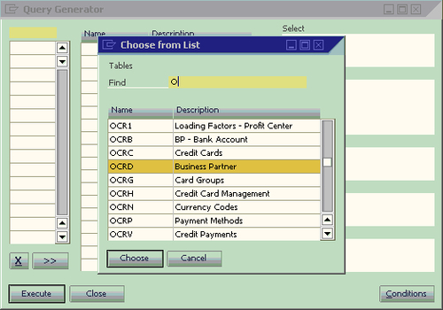
The set of table names will then show up. You could type any letters in the Find textbox to bring up the table names starting with that letter. In the example, you could find that the letter O is typed in. All tables starting with O would be on the top list. You could either use the scroll bar or page up/down key to find the tables you are looking for.
You'll remember we discussed the importance of the Data Dictionary in the previous chapter. Without the dictionary, it might be too hard to find which tables you need. If Table References is available, you could easily find the table quickly. For the sake of time, if you already know the names then you could just type in the full table names.
However, here is still one of the best places to find all commonly used tables for SAP Business One in case the help file is not available to you. In this less than ideal case, you probably need to go through the table name list quite a few times to become familiar with them.
In the example screenshot, the highlighted table OCRD (Business Partner table) will be selected when you click Choose:
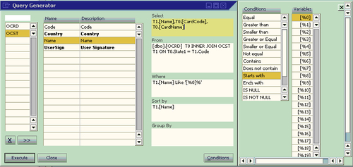
You may select more than one table in the same way as the first table was selected. In the screenshot you just saw, the OCST (State table) has also been selected. If you selected the wrong table or changed your mind, the X button here could be used to remove it from the list.
After the table selection, you would see that the middle part of the form shows you the fields from the highlighted table in alphabetical order. The right part shows the query component when you double-click the field name or table names on a proper box.
Under Select, three fields are selected from two tables. Under From, the table names are automatically shown with the default alias T0 and T1. The default link by system is also shown. If the link is not correct, you can manually fix it.
Under Where, you can choose any fields to restrict the query result. Here, T1.[Name] has been selected for the purpose of bringing the Business Partner according to the State/Province names.
You may notice that there is an additional form shown. This appears after clicking on the Conditions button. You may find 12 conditional formulas from the form that can be selected. The Variables part allows you to select variable as [%0], [%1], and so on. The percent sign plus a number represents a variable for SQL query in SAP Business One. It can allow the user to select or input values during query execution.
In the last example, Start With formula plus [%0] variable gives the result as T1.[Name] like '[%0]'. The additional % on the right of [%0] is a manual input wildcard character that can be used as a suffix to match any string of zero or more characters.
Under Sort, T1.[Name] is also selected to allow query results to be sorted by State/Province names.
When all the required information has been selected, click on Execute. Then the following form Query—Selection Criteria will pop up for you to input any letters:

In the previous example, a letter Y has been entered. That means you will get the query result with all business partner code and names from the state/province with the name starting with Y.
The result looks like the next screenshot:

If this query could be used later, click on Save near the bottom to save your query. It might be saved under any query categories with the name you entered. The topic regarding query saving will be discussed in detail later.
The Reverse Table button at the bottom of the form is used to help you choose to display the table either from right-to-left or from left-to-right. This is because unlike English, some of the other languages may not start from left-to-right, but in reverse order.
You may notice that all query script from different sections of the generator has been linked together for you. Remember, you do not need to write any single statement. This is such a good gift for you to reduce your learning curve in terms of query learning. Do not waste this valuable resource!
Query wizard is the second tool to be discussed in this chapter. It is similar to query generator. We are going to compare both tools later in the book.
Query Wizard enables easy access to the database and an easy way of building user-defined reports. It is designed for data retrieval/selection only. You are not able to do any DML queries such as updates, insert, or delete. This menu item can be accessed from Tools | Queries | Query Wizard.
With this tool, you can do the following:
- Create queries through five steps from a fixed set of tables from SAP Business One
- Access all data in those tables and get help from tips on each step
- Create individual reports without writing any single query statements
The first step is very simple. After you click on Query Wizard menu item, you get the first screen that simply tells you: This wizard will guide you step-by-step through the definition of parameters required for a query. The screenshot is omitted here since it is nothing but a splash screen for you to know you are starting this wizard.
The second step is similar to the left part in Query Generator. You can select as many tables as you need. However, you must try to minimize the number of tables for system performance and query efficiency.
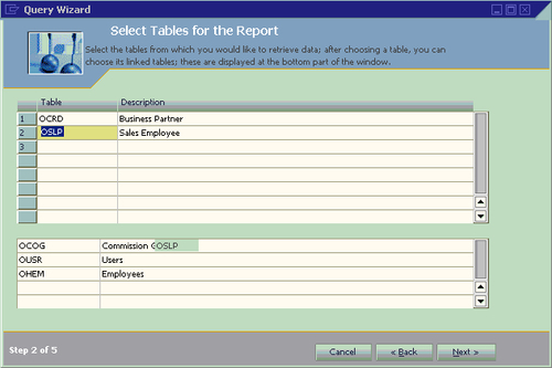
In the example screenshot you just saw, you may find that the first table selected is OCRD (Business Partner table). The second table selected is OSLP (Sales Employee table). Each table selected is placed in a separate row in the window. The second column displays the full description of the tables.
One thing here is, it is noticeably better than Query Generator. When you select any table, it automatically shows all linked tables under the lower part of the form. You will then find it very convenient to just choose the necessary tables by double-clicking.
This process applies to all tables selected in the upper part of the form.
A linked table list in the lower part of the form changes when you highlight different tables from the upper part of the form.
Step 3 in Query Wizard has the same function as the middle part of Query Generator. In addition, you have more options to select fields.
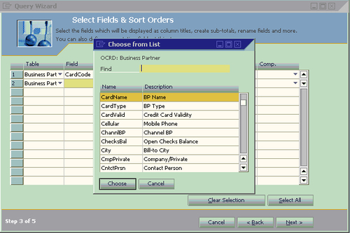
You may tab out the Field column to bring up Choose from list from the selected table. It is just like when you selected tables from both tools. You may type in any letters on the Find textbox to search your requested fields. There are two columns on the list:
- Name: Field names
- Description: Field description
As you know from the previous chapter, you can get all field information from the Table References for SAP Business One in advance. If that is not available to you, this might be the second best place to find all commonly used field information. You will probably need to go through them many times before you can reach frequently used fields at ease.
You can type the letter C to bring the field names starting with C on top of the list, so that you can get to the fields quicker. Or, you may not need to type any letters. Just use the mouse or page down to browse through the list in order to become familiar with those fields.
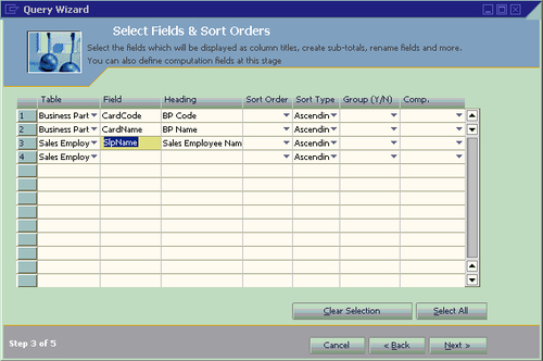
From the previous screenshot, you can see that two fields in OCRD have been selected. Another field from OSLP has also been selected. They are:
- CardCode: Business Partner Code from OCRD
- CardName: Business Partner Name from OCRD
- SlpName: Sales Employee Name from OSLP
The third column, Heading, displays the field description by default. You can change them to anything you want such as Customer Name instead of BP Name. It will show on the top of the query result screen as a column heading.
The fourth column, Sort Order, uses an integer (1, 2, 3) to set the sort priority; you can assign any orders to the field you have selected.
The fifth column defines the sort type as Ascending or Descending.
The sixth column allows you to set the group on any fields you would like to add. You just need to select Y for the field you would like it to be grouped to. If you have not selected this, the default value would be N.
The last column in the previous screenshot, Comp., offers six computation options:
- Total Records: Displays the number of records retrieved
- Total Distinct Records: Displays the number of distinct records retrieved
- Amount: Displays the sum of the values for numeric field in the retrieved records
- Average: Calculates and displays the average of the values of that field in the retrieved records
- Minimum: Displays the smallest value of this field from within the retrieved records
- Maximum: Displays the largest value of this field from within the retrieved records
Step 4 is for defining the conditions and relations for retrieving data. Both conditions and relations are based on the database structure and logic.
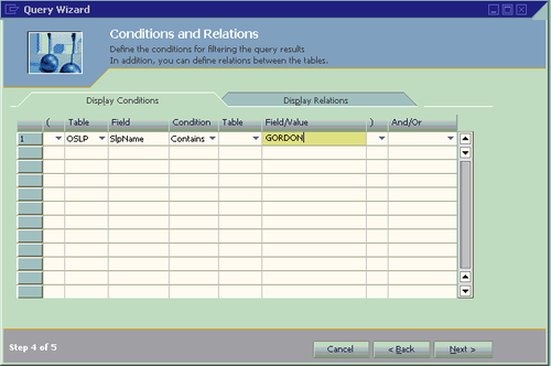
For the previous example, it is the Display Conditions tab. You can see the condition entered is Sales Employee's name, which contains Gordon.
You may select ( or ) on these two tabs to define the priority sequence of the conditions. You may also select And/Or to define complex conditions.
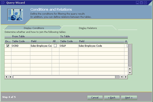
The other tab is for Display Relations. Under this tab, you will find the first column's checkbox, Execute. It applies the defined relationship between the tables that appear in the row. When this checkbox is selected, SAP Business One adds another condition. This means that the records you want to retrieve must comply with the conditions defined on the Define Conditions tab and with the added condition.
When you complete all Conditions and Relations, clicking on Next will bring you to the final step, which shows you the Query script created by the system that applies all of your selections.
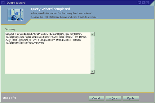
You may review the query to check if it is all you need. If you find that it did not include all conditions, you can go back to edit some of them in the previous steps.
In the example case, there are no problems. Click Finish to bring up the query result window.
You can find all Business Partner Codes and Names under the selected State/Province from the query results.
Like Query Generator, if the query is useful, you can click Save to save your query. The topic regarding query saving will be discussed in the Creating and saving user queries section of the next chapter.

Note
There is a video tutorial available for Query Wizard by SAP. You can find it here: http://www.youtube.com/watch?v=xaLO_4JnG-E. From this video, you will have additional information in a classroom-like instruction for the topic here.
Query Wizard overview
Query Wizard enables easy access to the database and an easy way of building user-defined reports. It is designed for data retrieval/selection only. You are not able to do any DML queries such as updates, insert, or delete. This menu item can be accessed from Tools | Queries | Query Wizard.
With this tool, you can do the following:
- Create queries through five steps from a fixed set of tables from SAP Business One
- Access all data in those tables and get help from tips on each step
- Create individual reports without writing any single query statements
The first step is very simple. After you click on Query Wizard menu item, you get the first screen that simply tells you: This wizard will guide you step-by-step through the definition of parameters required for a query. The screenshot is omitted here since it is nothing but a splash screen for you to know you are starting this wizard.
The second step is similar to the left part in Query Generator. You can select as many tables as you need. However, you must try to minimize the number of tables for system performance and query efficiency.
In the example screenshot you just saw, you may find that the first table selected is OCRD (Business Partner table). The second table selected is OSLP (Sales Employee table). Each table selected is placed in a separate row in the window. The second column displays the full description of the tables.
One thing here is, it is noticeably better than Query Generator. When you select any table, it automatically shows all linked tables under the lower part of the form. You will then find it very convenient to just choose the necessary tables by double-clicking.
This process applies to all tables selected in the upper part of the form.
A linked table list in the lower part of the form changes when you highlight different tables from the upper part of the form.
Step 3 in Query Wizard has the same function as the middle part of Query Generator. In addition, you have more options to select fields.
You may tab out the Field column to bring up Choose from list from the selected table. It is just like when you selected tables from both tools. You may type in any letters on the Find textbox to search your requested fields. There are two columns on the list:
- Name: Field names
- Description: Field description
As you know from the previous chapter, you can get all field information from the Table References for SAP Business One in advance. If that is not available to you, this might be the second best place to find all commonly used field information. You will probably need to go through them many times before you can reach frequently used fields at ease.
You can type the letter C to bring the field names starting with C on top of the list, so that you can get to the fields quicker. Or, you may not need to type any letters. Just use the mouse or page down to browse through the list in order to become familiar with those fields.
From the previous screenshot, you can see that two fields in OCRD have been selected. Another field from OSLP has also been selected. They are:
- CardCode: Business Partner Code from OCRD
- CardName: Business Partner Name from OCRD
- SlpName: Sales Employee Name from OSLP
The third column, Heading, displays the field description by default. You can change them to anything you want such as Customer Name instead of BP Name. It will show on the top of the query result screen as a column heading.
The fourth column, Sort Order, uses an integer (1, 2, 3) to set the sort priority; you can assign any orders to the field you have selected.
The fifth column defines the sort type as Ascending or Descending.
The sixth column allows you to set the group on any fields you would like to add. You just need to select Y for the field you would like it to be grouped to. If you have not selected this, the default value would be N.
The last column in the previous screenshot, Comp., offers six computation options:
- Total Records: Displays the number of records retrieved
- Total Distinct Records: Displays the number of distinct records retrieved
- Amount: Displays the sum of the values for numeric field in the retrieved records
- Average: Calculates and displays the average of the values of that field in the retrieved records
- Minimum: Displays the smallest value of this field from within the retrieved records
- Maximum: Displays the largest value of this field from within the retrieved records
Step 4 is for defining the conditions and relations for retrieving data. Both conditions and relations are based on the database structure and logic.
For the previous example, it is the Display Conditions tab. You can see the condition entered is Sales Employee's name, which contains Gordon.
You may select ( or ) on these two tabs to define the priority sequence of the conditions. You may also select And/Or to define complex conditions.
The other tab is for Display Relations. Under this tab, you will find the first column's checkbox, Execute. It applies the defined relationship between the tables that appear in the row. When this checkbox is selected, SAP Business One adds another condition. This means that the records you want to retrieve must comply with the conditions defined on the Define Conditions tab and with the added condition.
When you complete all Conditions and Relations, clicking on Next will bring you to the final step, which shows you the Query script created by the system that applies all of your selections.
You may review the query to check if it is all you need. If you find that it did not include all conditions, you can go back to edit some of them in the previous steps.
In the example case, there are no problems. Click Finish to bring up the query result window.
You can find all Business Partner Codes and Names under the selected State/Province from the query results.
Like Query Generator, if the query is useful, you can click Save to save your query. The topic regarding query saving will be discussed in the Creating and saving user queries section of the next chapter.
Note
There is a video tutorial available for Query Wizard by SAP. You can find it here: http://www.youtube.com/watch?v=xaLO_4JnG-E. From this video, you will have additional information in a classroom-like instruction for the topic here.
Step 1—Splash screen
The first step is very simple. After you click on Query Wizard menu item, you get the first screen that simply tells you: This wizard will guide you step-by-step through the definition of parameters required for a query. The screenshot is omitted here since it is nothing but a splash screen for you to know you are starting this wizard.
The second step is similar to the left part in Query Generator. You can select as many tables as you need. However, you must try to minimize the number of tables for system performance and query efficiency.
In the example screenshot you just saw, you may find that the first table selected is OCRD (Business Partner table). The second table selected is OSLP (Sales Employee table). Each table selected is placed in a separate row in the window. The second column displays the full description of the tables.
One thing here is, it is noticeably better than Query Generator. When you select any table, it automatically shows all linked tables under the lower part of the form. You will then find it very convenient to just choose the necessary tables by double-clicking.
This process applies to all tables selected in the upper part of the form.
A linked table list in the lower part of the form changes when you highlight different tables from the upper part of the form.
Step 3 in Query Wizard has the same function as the middle part of Query Generator. In addition, you have more options to select fields.
You may tab out the Field column to bring up Choose from list from the selected table. It is just like when you selected tables from both tools. You may type in any letters on the Find textbox to search your requested fields. There are two columns on the list:
- Name: Field names
- Description: Field description
As you know from the previous chapter, you can get all field information from the Table References for SAP Business One in advance. If that is not available to you, this might be the second best place to find all commonly used field information. You will probably need to go through them many times before you can reach frequently used fields at ease.
You can type the letter C to bring the field names starting with C on top of the list, so that you can get to the fields quicker. Or, you may not need to type any letters. Just use the mouse or page down to browse through the list in order to become familiar with those fields.
From the previous screenshot, you can see that two fields in OCRD have been selected. Another field from OSLP has also been selected. They are:
- CardCode: Business Partner Code from OCRD
- CardName: Business Partner Name from OCRD
- SlpName: Sales Employee Name from OSLP
The third column, Heading, displays the field description by default. You can change them to anything you want such as Customer Name instead of BP Name. It will show on the top of the query result screen as a column heading.
The fourth column, Sort Order, uses an integer (1, 2, 3) to set the sort priority; you can assign any orders to the field you have selected.
The fifth column defines the sort type as Ascending or Descending.
The sixth column allows you to set the group on any fields you would like to add. You just need to select Y for the field you would like it to be grouped to. If you have not selected this, the default value would be N.
The last column in the previous screenshot, Comp., offers six computation options:
- Total Records: Displays the number of records retrieved
- Total Distinct Records: Displays the number of distinct records retrieved
- Amount: Displays the sum of the values for numeric field in the retrieved records
- Average: Calculates and displays the average of the values of that field in the retrieved records
- Minimum: Displays the smallest value of this field from within the retrieved records
- Maximum: Displays the largest value of this field from within the retrieved records
Step 4 is for defining the conditions and relations for retrieving data. Both conditions and relations are based on the database structure and logic.
For the previous example, it is the Display Conditions tab. You can see the condition entered is Sales Employee's name, which contains Gordon.
You may select ( or ) on these two tabs to define the priority sequence of the conditions. You may also select And/Or to define complex conditions.
The other tab is for Display Relations. Under this tab, you will find the first column's checkbox, Execute. It applies the defined relationship between the tables that appear in the row. When this checkbox is selected, SAP Business One adds another condition. This means that the records you want to retrieve must comply with the conditions defined on the Define Conditions tab and with the added condition.
When you complete all Conditions and Relations, clicking on Next will bring you to the final step, which shows you the Query script created by the system that applies all of your selections.
You may review the query to check if it is all you need. If you find that it did not include all conditions, you can go back to edit some of them in the previous steps.
In the example case, there are no problems. Click Finish to bring up the query result window.
You can find all Business Partner Codes and Names under the selected State/Province from the query results.
Like Query Generator, if the query is useful, you can click Save to save your query. The topic regarding query saving will be discussed in the Creating and saving user queries section of the next chapter.
Note
There is a video tutorial available for Query Wizard by SAP. You can find it here: http://www.youtube.com/watch?v=xaLO_4JnG-E. From this video, you will have additional information in a classroom-like instruction for the topic here.
Step 2—Select tables for the report
The second step is similar to the left part in Query Generator. You can select as many tables as you need. However, you must try to minimize the number of tables for system performance and query efficiency.
In the example screenshot you just saw, you may find that the first table selected is OCRD (Business Partner table). The second table selected is OSLP (Sales Employee table). Each table selected is placed in a separate row in the window. The second column displays the full description of the tables.
One thing here is, it is noticeably better than Query Generator. When you select any table, it automatically shows all linked tables under the lower part of the form. You will then find it very convenient to just choose the necessary tables by double-clicking.
This process applies to all tables selected in the upper part of the form.
A linked table list in the lower part of the form changes when you highlight different tables from the upper part of the form.
Step 3 in Query Wizard has the same function as the middle part of Query Generator. In addition, you have more options to select fields.
You may tab out the Field column to bring up Choose from list from the selected table. It is just like when you selected tables from both tools. You may type in any letters on the Find textbox to search your requested fields. There are two columns on the list:
- Name: Field names
- Description: Field description
As you know from the previous chapter, you can get all field information from the Table References for SAP Business One in advance. If that is not available to you, this might be the second best place to find all commonly used field information. You will probably need to go through them many times before you can reach frequently used fields at ease.
You can type the letter C to bring the field names starting with C on top of the list, so that you can get to the fields quicker. Or, you may not need to type any letters. Just use the mouse or page down to browse through the list in order to become familiar with those fields.
From the previous screenshot, you can see that two fields in OCRD have been selected. Another field from OSLP has also been selected. They are:
- CardCode: Business Partner Code from OCRD
- CardName: Business Partner Name from OCRD
- SlpName: Sales Employee Name from OSLP
The third column, Heading, displays the field description by default. You can change them to anything you want such as Customer Name instead of BP Name. It will show on the top of the query result screen as a column heading.
The fourth column, Sort Order, uses an integer (1, 2, 3) to set the sort priority; you can assign any orders to the field you have selected.
The fifth column defines the sort type as Ascending or Descending.
The sixth column allows you to set the group on any fields you would like to add. You just need to select Y for the field you would like it to be grouped to. If you have not selected this, the default value would be N.
The last column in the previous screenshot, Comp., offers six computation options:
- Total Records: Displays the number of records retrieved
- Total Distinct Records: Displays the number of distinct records retrieved
- Amount: Displays the sum of the values for numeric field in the retrieved records
- Average: Calculates and displays the average of the values of that field in the retrieved records
- Minimum: Displays the smallest value of this field from within the retrieved records
- Maximum: Displays the largest value of this field from within the retrieved records
Step 4 is for defining the conditions and relations for retrieving data. Both conditions and relations are based on the database structure and logic.
For the previous example, it is the Display Conditions tab. You can see the condition entered is Sales Employee's name, which contains Gordon.
You may select ( or ) on these two tabs to define the priority sequence of the conditions. You may also select And/Or to define complex conditions.
The other tab is for Display Relations. Under this tab, you will find the first column's checkbox, Execute. It applies the defined relationship between the tables that appear in the row. When this checkbox is selected, SAP Business One adds another condition. This means that the records you want to retrieve must comply with the conditions defined on the Define Conditions tab and with the added condition.
When you complete all Conditions and Relations, clicking on Next will bring you to the final step, which shows you the Query script created by the system that applies all of your selections.
You may review the query to check if it is all you need. If you find that it did not include all conditions, you can go back to edit some of them in the previous steps.
In the example case, there are no problems. Click Finish to bring up the query result window.
You can find all Business Partner Codes and Names under the selected State/Province from the query results.
Like Query Generator, if the query is useful, you can click Save to save your query. The topic regarding query saving will be discussed in the Creating and saving user queries section of the next chapter.
Note
There is a video tutorial available for Query Wizard by SAP. You can find it here: http://www.youtube.com/watch?v=xaLO_4JnG-E. From this video, you will have additional information in a classroom-like instruction for the topic here.
Step 3—Select fields and sort orders
Step 3 in Query Wizard has the same function as the middle part of Query Generator. In addition, you have more options to select fields.
You may tab out the Field column to bring up Choose from list from the selected table. It is just like when you selected tables from both tools. You may type in any letters on the Find textbox to search your requested fields. There are two columns on the list:
- Name: Field names
- Description: Field description
As you know from the previous chapter, you can get all field information from the Table References for SAP Business One in advance. If that is not available to you, this might be the second best place to find all commonly used field information. You will probably need to go through them many times before you can reach frequently used fields at ease.
You can type the letter C to bring the field names starting with C on top of the list, so that you can get to the fields quicker. Or, you may not need to type any letters. Just use the mouse or page down to browse through the list in order to become familiar with those fields.
From the previous screenshot, you can see that two fields in OCRD have been selected. Another field from OSLP has also been selected. They are:
- CardCode: Business Partner Code from OCRD
- CardName: Business Partner Name from OCRD
- SlpName: Sales Employee Name from OSLP
The third column, Heading, displays the field description by default. You can change them to anything you want such as Customer Name instead of BP Name. It will show on the top of the query result screen as a column heading.
The fourth column, Sort Order, uses an integer (1, 2, 3) to set the sort priority; you can assign any orders to the field you have selected.
The fifth column defines the sort type as Ascending or Descending.
The sixth column allows you to set the group on any fields you would like to add. You just need to select Y for the field you would like it to be grouped to. If you have not selected this, the default value would be N.
The last column in the previous screenshot, Comp., offers six computation options:
- Total Records: Displays the number of records retrieved
- Total Distinct Records: Displays the number of distinct records retrieved
- Amount: Displays the sum of the values for numeric field in the retrieved records
- Average: Calculates and displays the average of the values of that field in the retrieved records
- Minimum: Displays the smallest value of this field from within the retrieved records
- Maximum: Displays the largest value of this field from within the retrieved records
Step 4 is for defining the conditions and relations for retrieving data. Both conditions and relations are based on the database structure and logic.
For the previous example, it is the Display Conditions tab. You can see the condition entered is Sales Employee's name, which contains Gordon.
You may select ( or ) on these two tabs to define the priority sequence of the conditions. You may also select And/Or to define complex conditions.
The other tab is for Display Relations. Under this tab, you will find the first column's checkbox, Execute. It applies the defined relationship between the tables that appear in the row. When this checkbox is selected, SAP Business One adds another condition. This means that the records you want to retrieve must comply with the conditions defined on the Define Conditions tab and with the added condition.
When you complete all Conditions and Relations, clicking on Next will bring you to the final step, which shows you the Query script created by the system that applies all of your selections.
You may review the query to check if it is all you need. If you find that it did not include all conditions, you can go back to edit some of them in the previous steps.
In the example case, there are no problems. Click Finish to bring up the query result window.
You can find all Business Partner Codes and Names under the selected State/Province from the query results.
Like Query Generator, if the query is useful, you can click Save to save your query. The topic regarding query saving will be discussed in the Creating and saving user queries section of the next chapter.
Note
There is a video tutorial available for Query Wizard by SAP. You can find it here: http://www.youtube.com/watch?v=xaLO_4JnG-E. From this video, you will have additional information in a classroom-like instruction for the topic here.
Step 4—Conditions and relations
Step 4 is for defining the conditions and relations for retrieving data. Both conditions and relations are based on the database structure and logic.
For the previous example, it is the Display Conditions tab. You can see the condition entered is Sales Employee's name, which contains Gordon.
You may select ( or ) on these two tabs to define the priority sequence of the conditions. You may also select And/Or to define complex conditions.
The other tab is for Display Relations. Under this tab, you will find the first column's checkbox, Execute. It applies the defined relationship between the tables that appear in the row. When this checkbox is selected, SAP Business One adds another condition. This means that the records you want to retrieve must comply with the conditions defined on the Define Conditions tab and with the added condition.
When you complete all Conditions and Relations, clicking on Next will bring you to the final step, which shows you the Query script created by the system that applies all of your selections.
You may review the query to check if it is all you need. If you find that it did not include all conditions, you can go back to edit some of them in the previous steps.
In the example case, there are no problems. Click Finish to bring up the query result window.
You can find all Business Partner Codes and Names under the selected State/Province from the query results.
Like Query Generator, if the query is useful, you can click Save to save your query. The topic regarding query saving will be discussed in the Creating and saving user queries section of the next chapter.
Note
There is a video tutorial available for Query Wizard by SAP. You can find it here: http://www.youtube.com/watch?v=xaLO_4JnG-E. From this video, you will have additional information in a classroom-like instruction for the topic here.
Step 5—Query wizard completion
When you complete all Conditions and Relations, clicking on Next will bring you to the final step, which shows you the Query script created by the system that applies all of your selections.
You may review the query to check if it is all you need. If you find that it did not include all conditions, you can go back to edit some of them in the previous steps.
In the example case, there are no problems. Click Finish to bring up the query result window.
You can find all Business Partner Codes and Names under the selected State/Province from the query results.
Like Query Generator, if the query is useful, you can click Save to save your query. The topic regarding query saving will be discussed in the Creating and saving user queries section of the next chapter.
Note
There is a video tutorial available for Query Wizard by SAP. You can find it here: http://www.youtube.com/watch?v=xaLO_4JnG-E. From this video, you will have additional information in a classroom-like instruction for the topic here.
When you go through the first part of the chapter, you have probably already noticed the differences between the Query Generator and Query Wizard tools.
You will find the summarized differences here to clarify any doubts you may have.
The first tool, Query Generator, is one of the simplest tools for building SQL Queries. It just uses one simple User Interface (UI) for you to create queries. You can start to use it whenever you wish to find the tables, fields, and their relationship.
The second tool, Query Wizard, has added five steps with different forms, so that you can find the table relationship more easily. Also, finding fields becomes much easier because you have the option to bring up Choose from list.
Here is the list showing the similarities between these two tools:
- There is no need to write full query statements
- Allows selection of tables and fields
- Prohibits updating data
- Uses the mouse alone to add conditions
|
Differences |
Query Generator |
Query Wizard |
|---|---|---|
|
Single step User Interface Requires more tables and fields knowledge Less help and tips Field level selection is basic |
Multiple steps User Interface Requires less tables and fields knowledge More help and tips Field level selection is sophisticated |
In summary, the Query Generator is designed to get quick results in a single step, while Query Wizard is more concentrated on step-by-step instructions to help you build queries with clear selection in different phases.
I prefer the Query Generator over the Query Wizard because I am familiar with all tables and fields. To me, the simpler the steps, the better. To a beginner, I would suggest you try Query Wizard because it gives you more power to select different tables and fields. You will also be provided with more helpful tips.
Besides Query Generator and Query Wizard, there is another powerful tool for you to learn SQL Query in SAP Business One. That is: System Queries.
System queries enable you to generate additional reports and retrieve data that is not available by running the other reports. You may access system queries either from the different modules—in each module the relevant system queries appear as entries under report menu, identified with the icon ? or by choosing them from Tools | Queries | System Queries.
The following screenshot shows you the names of all the available system queries. You may find as many as 18 queries here. Most queries are related to finance and banking.
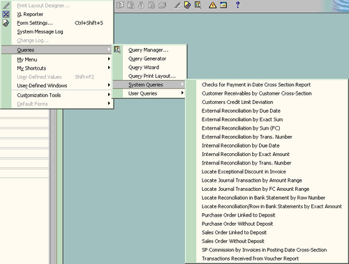
You can see the query results from one of the system queries: Purchase Order Linked to Deposit.
The result is actually empty because there is no deposit linked to the purchase order in the database. You would like this result, wouldn't you?
What you need to know is the top part of the query result. You will see there is a Left Arrow (Show icon) there. When you click on the arrow, you will get the full body of the query statements.

As soon as you click on the Left Arrow icon, it will become Down Arrow (Hide icon). You will notice there are two additional icons displayed. One is Pencil Only. The other is a Pencil with Cross. All query statements are shown as well.
This is only available if you run those system queries under the tools menu instead of each module under report.
When you click on the Pencil Only icon, the background of the query statement area will become yellow instead of grey. You are now able to modify the query for your own use.
When you finish editing, you may click the other icon (Pencil with Cross). That will change back to the read only mode of the query body.

If you are interested, here is the complete statement of this query:
DECLARE @Factor as numeric(1,0)

SELECT @Factor =
CASE (SELECT TOP 1 DispPosDeb FROM OADM)
 WHEN 'N' THEN 1 ELSE -1
END

SELECT T0.CardCode,
T0.CardName,
T0.Balance,
T0.CreditLine,
(T0.CreditLine + @Factor*T0.Balance) "Deviation"

FROM OCRD T0
WHERE (select T0.CreditLine + @Factor*T0.Balance) < 0 AND T0.CardType = 'C'
If you come across any difficulties in creating your query later, you can always come back to system queries to find some useful tips.
In this chapter, you have learned about the following tools for creating or using SQL queries in SAP Business One:
- Query Generator
- Query wizard
- System queries
You have also learned the differences between Query generator and Query wizard. This is a good start for your progress in mastering SQL Queries for SAP Business One.
By practicing these tools, you could have better understanding of the tables and table relationship within SAP Business One. Some of the system queries will give you more hints than others regarding how to create the correct query.
If you are a beginner, you may need to try those tools quite a few times. Only when you feel comfortable in creating simple queries – without problems – with these tools, will you build a solid foundation to create more sophisticated queries. In order to benefit from Business Intelligence, it would be better to try to master these tools to as high a level as possible. To learn the details of each statement and the complicated syntax, continue to read the following chapters.
In the next chapter, you will learn about the Query Manager and all the commonly used statements and functions, one by one, and in detail.
In the previous chapter, you learned about two basic tools, Query Generator and Query Wizard. Meanwhile, you also learned about system queries so that you can create or use queries with these tools. However, those tools have certain limitations.
The most inconvenient limitation is that only a fixed set of tables is available to you with these tools. For example, the table list does not show all tables in the database. When the queries become complicated, these tools may not work for you.
You must be eager to know how to create queries freely without those restrictions. Do you have other ways of creating queries when you need to create them in complex logic? The answer is definitely: "Yes". This is the topic of this chapter.
This chapter illustrates the most important business intelligence tool for SAP Business One: Query Manager. You will learn how to manage your queries by creating, saving, and deleting them directly from the Query Manager. At the same time, you will learn how to organize your queries into categories. The detailed query statements, keywords, and functions will be presented to you as well.
In the first section, you will learn everything related to the Query Manager such as User Interface, including each button. The query categories for saved query will also be discussed. The next section will show you the most commonly used basic statements for queries one by one. All statements are fully explained. They cover the most frequently used statements. The last section covers the query functions, including the most commonly used functions or expressions.
The following screenshot shows you how to access this tool from the SAP Business One menu:

Just like the other query tools, Query Manager can be accessed through the first menu item under Tools | Queries.
You can also access it directly from the toolbar. The Query Manager icon can be found on the toolbar between the Form Settings and Message/Alert icons. This icon is shown in the previous screenshot on the left side of Query Manager.
In the Query Manager window, you can:
- Display all existing queries
- Create and save user queries
- Delete user queries
- Manage query categories
Query Manager is used for query management. All queries can be saved, edited, or deleted by using the Query Manager tool. It does not matter if the query is created by tools like Query Generator/Query Wizard, or by users directly from the query result windows.
This is the simplest function for the Query Manager. You can find all your saved queries or system queries through the Query Manager User interface.
The first text block on the top of the Query Manager can display the query name you have selected or allow you to type a query name for a new query before you save it.
The next text block below the query name can display the query category you have selected or allow you to type a query category name for a new query category before you save it through the Manage Category function.
The big window under these two boxes is the place to display all query categories and the query names for the expanded categories you have selected.
The first screenshot shows the system query names:

The second example shows the query categories plus the query names under expanded query categories:

You may notice that there are two different icons in front of each query category: the Down Arrow icon next to the General category and the Right Arrow icon next to System as well as other categories. The Down Arrow icons stand for the query categories that are expanded to display the query names under the categories. The Right Arrow icons refer to the query categories that are not expanded. When you click on the icon, the status will change from expanded to non-expanded or vice versa. To find a query under a specific category, you just need to click on the icon in front of the query category to expand it.
You can display any queries in two ways:
- The first way is from the Query Manager window directly. You can find the required query name and double-click on the name or you can click OK when you select a specific query name. The selected query will be displayed on the query result window with either method.
- The second way is bypassing the Query Manager window. You can also find the query name directly from Tools | Queries | User Queries. One click is good enough to bring up the query result window with this method.
The second method presents a limitation. If the query name is too long, it might be cut off when you display their names directly from the Tools menu. Or if you have special characters, it may not display them fully either. It is advisable to use shorter names for queries whenever possible. Avoid using special characters whenever possible.
Creating user queries can be done directly after you run any queries in order to bring up the query result window. The query you want to run can either be from query tools directly or selected from the Query Manager.
When you open the query result window by either of the methods mentioned earlier, you might be able to edit or create a query from scratch, if you have the right authorization. In case you don't have the user privilege, check with the Superuser in your company.
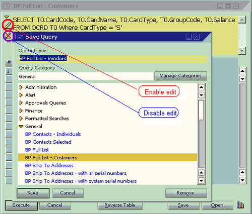
Once you have got proper user rights, you will be able to find two icons on the left screen beside the query script. They look like a pencil or a pencil with a red line cross. From the previous screenshot, you can find that the first icon is used for enabling edit queries and the second icon is the opposite, that is, to disable the editing ability. When you click on the pencil icon, you will have the power to write any queries to retrieve data from any tables in the database.
Unlike the other query tools, you have to write every single statement, keyword, column name, table name, function, and parameter on your own. The freedom to write query as you wish requires that you have both high level SQL query knowledge and SAP Business One database structure knowledge. If you find it is difficult, you need to go back to the previous chapter. Spend your time with the tools until you are ready.
To save your query, you just need to follow these steps:
- Click on Save. The Save Query window will show up.
- Select any categories from the list.
- Type in a proper query name.
- Click on Save under the bottom of the window.
Your query will be saved immediately with the previously mentioned steps.
The Save Query window is similar to the Query Manager window. Any query categories or query names displayed in the Query Manager window, will be displayed in the Save Query window too.
The following example shows that the existing query, BP Full List—Customer, has been edited. The new query can be saved by selecting the category General and selecting a query name to modify it to. The new name BP Full List—Vendors has been entered. After clicking on Save, this new query is saved under the General category. You can just type in the name if the name is not very long.
Note
Warning: Although you can write some DML queries such as UPDATE, DELETE, or INSERT in the query result windows, those DML queries have to be restricted to only your User Defined Tables (UDT). Even User Defined Field (UDF) in the system tables is not allowed to be updated by the SQL Query directly. You face great risk of losing your SAP support in case of any corruptions in your database, if you have directly updated system tables.
If you need to create a query from scratch without bringing up other queries, you can create an empty query such as SELECT '' and save it by a name Blank or Empty. If you run this query, you will see nothing in the query result but empty space that allows you to create a brand new query.
It is simple to delete a user query. You don't need to open the query to run it, but delete it from the Query Manager window directly. After you have selected the Query Manager from the menu or through the icon, you can select the query you want to delete. Click on the Remove button, and a warning message will popup to confirm that you want to delete the query. If you have not reached this point through a wrong mouse click, you can click on Yes to proceed. The query will be deleted from the database.
There is an alternative way to delete queries. That is to bring up the Save Query window by clicking Save under the query result window. Instead of saving queries, you may select any user queries to delete. Clicking on the Remove button is all you need to do.
After deleting queries, you can click on Cancel to return to the query result window.
Note
Be careful when you delete your query. There is no Undo function like some other applications. Once the query is deleted, there is no way to retrieve it unless you restore your entire database! A practical remedy is to copy and save all queries to a text document after you have created them. It will save you time whenever you find the queries have to be revised or deleted.
Categories are the folders for queries. They include categories for system queries and categories for user queries. You always get a default category called General when you have a new database. There is nothing else beside these system and general categories in the beginning. It is dependent on an administration user to create and maintain your queries with any categories you like.
If you only have few queries, categories may not be that important to you. However, this will change as soon as you have more saved queries. Good category management can save you tremendous time. You can maintain the categories with the same structure as the SAP Business One menu system. Any queries can be found quickly in this way.
Categories are similar to directories or folders in an operating system, with one exception. This is not a trivial exception. There is only one level for categories under the Query Manager. You don't have the option to create multi-level categories.
Tip
Due to the limitations of having only one level category, your plan to create categories should avoid any overlap structure. If your categories have not clearly divided the scope of your queries, you may face a dilemma in saving your new query to a proper category. When you try to find the saved queries in the future, it may actually increase your troubles in getting the right queries, instead of saving you time.
To manage categories, you can click Manage Category beside the second text box. After you click the button, a window with a title Create/Edit Categories will pop up like in the following screenshot:
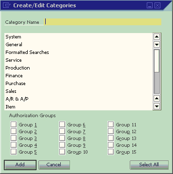
When this window pops up, it is always in Add mode. You can add a new category by typing any letters in the text box close to the top of window. Then click ADD. The new category will be added right away.
If you are not satisfied with the category name, it is very easy to edit it. Just select a category name when you are in the Add mode. The Add button will change to an Update button instantly, like the example in the following screenshot. A/R & A/P category is selected to be a candidate for update.

You can type in your preferred category name at this time. In the example, Gordon is typed in. When you click Update, the category name changes to Gordon instead of A/R & A/P.
The query names under the same category will not be affected when you are editing category names. Actually, this is the category ID to be used by the system. This category ID is not changed during your category name update.

After you click Update, the window is changed to find mode. The button is changed again from Update to OK. You can still select any categories just like in the Add mode. However, the button will not change to Update this time. It still shows OK.
To add another new category, you have to change the window mode to Add mode. This can be done through the menu item Data | Add, keyboard shortcut Ctrl+A or the icon on the toolbar.

The last button to be discussed is the Select All button. This button allows you to select all Authorization Groups. If you want to assign your query category to more than half of the authorization groups, it will be easier to click on this button first. Then you can deselect any groups. If you just assign to less than half of the groups, you can check them one by one. It will save you time compared with unchecking many boxes after Select All.
Whenever you have not selected all groups, the Select All button will be available. As soon as all groups are selected, the button will change to Clear All. The authorization groups are used for query report user authorizations. The details for query report user authorizations will be discussed in Chapter 5.
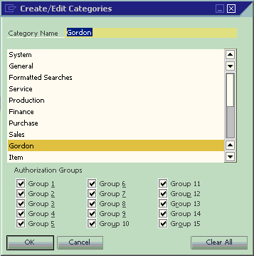
SQL queries comprise a statement, keyword, function, expression, and parameters. To see how commonly used query statements work, you can have a look at the following query example that includes most of the statements and some of the functions. The query contents and meaning of these query results will be discussed in the next chapter:
SELECT TOP 5 T0.ShortName 'Customer',
Max(T2.CardName) 'Customer Name',
SUM(ISNULL(T0.Debit,0) - ISNULL(T0.Credit,0)) as "Amount(LC)"
FROM dbo.JDT1 T0
INNER JOIN dbo.OJDT T1 ON T1.TransID = T0.TransID and T0.TransType IN (13,14)
INNER JOIN dbo.OCRD T2 ON T2.CardCode = T0.ShortName
WHERE t1.RefDate >= [%0] and t1.RefDate <= [%1]
GROUP BY T0.ShortName
HAVING SUM(ISNULL(T0.Debit,0) - ISNULL(T0.Credit,0)) > 0
ORDER BY SUM(ISNULL(T0.Debit,0) - ISNULL(T0.Credit,0)) DESC
This query can be used to return the top five customers for sales in any period based on the date range you selected. It includes most of the statements that are going to be discussed in this chapter.
Let us go through those statements or functions in Bold from the sample query one by one:
It is quite obvious from the meaning of the word that SELECT is used to display or retrieve data from certain data sources.
The SELECT statement is used to return data from a set of values or database tables.
The result is stored in a result table, called the result-set.
SELECT is one of the most commonly used Data Manipulation Language (DML) commands. It seems very simple. However, something important needs to be explained for this statement:
- The scope of the value that can be retrieved
- The numbers of columns to be included
- Column name descriptions
- Keywords followed to this statement
Here is a return value list that SELECT can be used for:
- A single value
- A group of values
- Return a single database table column
- Return a group of database table columns
- Return complete database table columns
- Used in a subquery
The simplest SELECT query would be just to get a constant or text without any additional statements. An example would be:
SELECT 'YES' AS 'Yes/No' or
SELECT 10 AS 'No.'
These queries will display Yes or 10 in one column when executed.
You may also use this statement to get a group of values. For example:
SELECT 'YES' AS 'Yes/No', 10 AS 'No.', 'This is an example' AS 'Content'
This query will display Yes, 10, This is an example in three columns named Yes/No, No., and Content when you execute it.
Some special uses of this statement to display a single value or group of values will be discussed in other chapters when we introduce more specific topics.
Please note the comma used above. Following the SELECT statement, each comma will define a new column to be displayed.
Tip
Do not forget to delete the last comma in a SELECT statement. This simple mistake is one of the most frequent problems for a query. It is mainly due to the fact that we are often used to copying columns in our queries, which include the comma, and forget to remove the last one before testing the query.
Similar to the single value SELECT, we can use it for a database table column. Here is an example:
SELECT CompnyName
FROM OADM
This simple example will retrieve your company name from table OADM.
The formal query should be this:
SELECT T0.CompnyName
FROM dbo.OADM T0
It is an important step to include Alias (T0) and Database Owner (dbo) for the table in the query. It will ensure the query's consistency and efficiency. This topic will be discussed in the FROM clause in more detail.
There is no big difference with the previous example. We can use the same principle to select multiple database table columns. For instance:
SELECT CompnyName, CompnyAddr, Country, Phone1
FROM OADM
This example will retrieve not only your company name, but also your company's address, country, and phone number from table OADM.
The formal query should be as follows:
SELECT T0.CompnyName, T0.CompnyAddr, T0.Country, T0.Phone1 FROM dbo.OADM T0
This is the simplest query to return all column values from table. That is:
SELECT *
FROM OADM
This example will retrieve every single column from table OADM. There is no need to assign alias to the query because this kind of query is usually a one-time only query. Here, * is a wildcard that represents everything in the table.
Note
Be careful when running SELECT * from a huge table such as JDT1. It may affect your system's performance! If you are not sure about the table size, it is safer for you to always include the WHERE clause with reasonable restrictions. Or you can run SELECT COUNT(*) FROM the table you want to query first. If the number is high, do not run it without a condition clause.
How many columns are suitable for a query? I don't think there are any standard answers. In my experience, I can only suggest to you: the shorter, the better.
Some people have the tendency to include all information in one report. This kind of request may even come from certain executives of the company's management.
One simple test would be a fair criterion. Can you fit the query result within the query result window? If you can, great; that would be a proper number of columns. If not, then I would strongly suggest you double check every column to see if you can cut one or more of them out.
If it is a query for alert, it needs even more special care. The column numbers in any alert queries have to be trimmed to the minimum. Otherwise, you may only get part of the result due to the query result size limitation. You will get more explanation for this issue in the chapter for alert queries.
If you are requested to create super long and wide queries, explain the consequences to the person in charge. Sometimes, they can change their mind depending on the way you communicate with them. In my experience, if a print out report cannot be handled within the width of a page, it might make the report difficult to read. Show the result to a non-technical person. It is easily understandable when you can bring the first hand output to the report readers.
Column names usually come directly from column descriptions, if you have not reassigned them in the query. You can, however, change them to make the query result more useful for special cases. Some people use this method to translate the description into their local language. Some people use it to make the column description more clear.
For some of the value-only columns or formula columns it is mandatory to assign descriptions, otherwise the column headings would be empty. This not only looks unprofessional, but you will also have no way to export the query results to Excel for those columns without the description.
You can use single or double quotation marks for the description. If the description has only one word, you can even omit the quotation mark. The syntax is shown next:
[ColumnName] AS 'Column Description Here'
You can omit AS, so that you just keep [ColumnName] 'Description Here'. However, whenever possible, you should keep the AS to make the query script more consistent.
A DISTINCT clause is used for getting rid of duplicated records to return only distinct (different) values.
The syntax of this clause is:
SELECT DISTINCT column_name(s)
FROM table_name(s)
column_name and table_name are self explanatory. They represent column name and table name respectively. There will be no additional denotation for these two clauses in this book. A DISTINCT clause is always the first one after the SELECT statement. It is optional. When you specify Distinct in the query, it will not allow any identical rows in the query result. All lines are unique from each other.
Some users claim this clause may still allow duplicate rows. This can never be true. The fact is: although most of the values are the same between two lines, the query results always include at least one column, which contains the different values. Those columns have to be taken out in order to benefit from this clause. You cannot get both the DISTINCT working and some columns which have different values within the scope you selected.
A TOP clause is used to specify the maximum number of records to return in a query result-set. It is usually used together with the Order By clause at the end of the query.
The syntax of the clause is as follows:
SELECT TOP (number)|percent[with ties] column_name(s)
FROM table_name(s)
The query result can be the top 10 sales orders, for example. In this case, descending order must be used for the document amounts. Or you may get the top 20 percent purchase invoices, if you specify the TOP by percentage. When you use percentage, you need to write
20 percent instead of 20% after SELECT TOP.
The WITH TIES option specifies the additional rows that need to be returned from the base result set with the same value in the ORDER BY columns appearing at the end of the TOP n (PERCENT) rows. TOP...WITH TIES can be specified only if an ORDER BY clause is specified.
Microsoft suggests SELECT TOP (n) with parentheses. It is better to follow the suggestion to be safe for the query results.
It is very clear that FROM means where to find the data. A FROM clause is actually not a standalone statement since it must be used with SELECT. Most queries need this clause because to only assign a fixed value or a group of values would not be very useful. However, this is one of the most often misused parts of SQL queries. More discussion is needed on this clause.
A FROM clause can be followed by the data sources mentioned next:
Tip
If you have read through Chapter 1, SAP Business One Query Users and Query Basic, you should understand the concept of Table and Table Relationships. If you directly jumped here bypassing that previous chapter, you may need to go back to check.
This is the simplest query including a FROM statement. A simple example:
SELECT Code, Name, Remarks FROM OUDP
This will only touch one table—OUDP. This table is for a department. You can get the Department Code, Department Name, and the Description from the query result.
The better format would be:
SELECT T0.Code, T0.Name, T0.Remarks FROM dbo.OUDP T0
Now, it is time to explain why those additional T0 and dbo are necessary here.
Actually, it may not make any difference if we only deal with this particular query and this query is only run by one user. However, that is not generally true. In most cases, we often have more than one table and more than one user to run the same query.
T0 here stands for an Alias of OUDP table. It is the standard convention and most frequently used alias. T means table. 0 is a sequence number. You can have T0, T1, T2, …until Tn. If you have 10 tables in the query, n would be equal to 9 for alias. This naming convention is convenient to use. You just need to name them in sequential numbers.
The syntax for table alias looks like this:
SELECT alias_table_name.column_name
FROM table_name [AS] alias_table_name
An alias table name can be anything, but usually it is the shortest possible one.
If a query is not created by query tools, it is not mandatory for alias to take the Tn sequence. You may just use A, B, C, …… to have one letter shorter than the standard way, or make them easier to remember. However, it is advisable that you follow the norm. It can save you time for maintaining your query in the long run.
The function for alias is mainly for saving resources. If no alias is defined, you have to enter the full table names for every single column in the query. Be careful when you are using alias; you should use alias exclusively throughout your query. You are not allowed to mix them with the actual table name. In other words, you may only use alias or the actual table name, but you are not allowed to use them both in the same query.
The other added word dbo means Database Owner. This is a special database user. This user has implied permissions to perform all activities in the database. All tables of SAP Business One have the owner of dbo. It is useful to add dbo in front of a table name when you have more than one user running the query, but this is beyond the scope of the book. I will try to use the simplest method to give you a rough idea.
Query running needs an execution plan. A query execution plan (or query plan) outlines how the SQL Server query optimizer (query optimizer is too complicated to explain here, you just need to know it is a tool built into SQL server) actually ran (or will run) a specific query. There are typically a large number of alternate ways to execute a given query, with widely varying performance. When a query is submitted to the database, the query optimizer evaluates some of the different, correct possible plans for executing the query and returns what it considers the best alternative. This information is very valuable when it comes to finding out why a specific query is running slowly.
The hard fact is: no one can control this plan manually at runtime. Once a plan is created, it is reusable for the same user to run the query. If you are not entering dbo in front of the table name, the query will check every user who runs the query. A new plan may be added for every new user because the owner is not included in the query body. That might cause too much unnecessary burden to the database.
This is the category that most queries will be included in. One example may not be enough to show this clearly. You have two query examples to show. The first one is as follows:
SELECT Distinct T0.[DocNum], T1.DocNum, T0.[DocType], T0.[CardCode], T0.[CardName], T0.[UserSign], T0.[UserSign2], T1.[UserSign], T1.[UserSign2]
FROM dbo.ADOC T0
INNER JOIN dbo.ORIN T1 ON T0.DocNum = T1.DocNum
WHERE T0.[ObjType] = '14' AND T0.[UserSign2] != T1.[UserSign2]
This query links ADOC (Document History) and ORIN (Credit Memo Headers) tables to show the credit memo document number, document type, user information, and the change log user code for the credit memo. A detailed explanation can be found in the next chapter.
The second query example is as follows:
SELECT T1.CardCode as "CustCode", T1.CardName as "CustName", T2.SlpName, T1.DocNum "Incoming#", T1.DocDate, T1.DocTotal as "Payment Total", T4.DocNum as "Invoice#", T3.SumApplied as "Applied Total"
FROM dbo.OCRD T0
INNER JOIN dbo.ORCT T1 ON T0.CardCode = T1.CardCode
LEFT JOIN dbo.OSLP T2 ON T0.SlpCode = T2.SlpCode
INNER JOIN dbo.RCT2 T3 ON T3.DocNum = T1.DocNum
INNER JOIN dbo.OINV T4 ON T4.DocEntry = T3.DocENtry AND T3.InvType = '13'
WHERE T1.DocDate >= [%0] AND T1.DocDate <= [%1]
ORDER by T1.DocDate
This query links five tables OCRD (Business Partners), ORCT (Incoming Payment Headers), RCT2 (Incoming Payments—Invoices), OSLP (Sales Employees), and OINV (Invoice Headers) together. It shows customers' payment with invoice details. Again, the business case explanation is available in the next chapter.
Among the five links in the query, there are two different kinds of links. One is INNER JOIN. The other is LEFT JOIN; more explanation of these joins can be found later in the chapter.
When you link tables together, SQL Server just treats them as a view, or it acts as one big table. However, there is another way to add your tables into the query without linking them first. The syntax is similar to comma delimited columns. You simply need to enter a comma in between tables. In this case, table linking has to be done under the WHERE conditions.
Technically, the way of linking tables without joining is the most ideal method because you can get the minimum records out with the least database operations, if you are very good at database structure. However, like the difference between manual and automatic cameras, most people prefer automatic cameras because it is very convenient, especially if you do not have extensive training or extraordinary experience, and the ideal manual control may not help you get a better picture!
I always refuse to create queries without joining the tables first. Comma-separated table query is too dangerous. If you have the wrong conditions defined in the WHERE clause, you may end up with countless loops. In the worst case scenario, it may lock your system up. On the contrary, if you link all tables together, the worst case scenario would be no results because of a bad link or bad conditions.
In other words, if you want to add all tables' linking conditions under the WHERE clause, you are giving yourself an unnecessary burden in making sure they are correct. Those verifications have to be done manually.
Whenever possible, you are better to avoid using comma separated table queries. In most cases, it may use more resources and put you at a higher risk of system instability.
You have learned the FROM statement. With this statement, you know that more than one table can be put into one query.
In most cases, those additional tables should be linked together. The reason we need to link tables before the WHERE clause has been discussed in the previous paragraph. To link those extra tables, JOIN is used to combine rows from multiple tables.
A join is performed whenever two or more tables are listed in the FROM clause of a SQL statement without using a comma to separate them. Joined tables must include at least one common column in both tables that contain comparable data. Column names across tables don't have to be the same. But if we have the same name columns to join with correct relation, use them first.
There are different types of JOIN statements to be discussed, listed as follows:
- Inner join
- Outer joins
- Self-join
One of the special join types is omitted from the list. This is called the Cross Join. This type of join can list all possible combinations of your linked tables. You may end up with 90,000 lines of huge output even if you have only 300 records in each table. I have no idea who can benefit from this Cross Join. They must be very special.
First, let's look at the most commonly used one.
An INNER JOIN is also called a Simple Join. It is the simplest table join. INNER JOIN is the default link type to join tables. You may even omit INNER to leave only JOIN. When you see JOIN without any words in front, it means INNER JOIN. In order to distinguish other types of JOIN, omission is not encouraged unless your query length is an issue that requires you to reduce your query to the minimum size.
An INNER JOIN syntax looks like the following:
SELECT T[0]|[1].column_name(s)
FROM table_name0 T0
INNER JOIN table_name1 T1
ON T0.column_name=T1.column_name
In an INNER JOIN statement, the link is defined by the keyword ON with common columns from each table to retrieve the matching records from those tables. To link two or more tables correctly, the linking columns are very important. INNER JOIN will select all rows from linked tables as long as there is a match between the columns you are matching on. If you forget the keyword ON in the joined table list, you will get an error message right away when you try to run the query.
The best way to link tables is by using the Key Columns such as the primary key or the foreign key. That is because Key Columns are usually indexed. That makes links easier and faster. In case there is no such columns' pair to link, care must be taken to select the best efficient common columns between tables. When you have more than one way to link, you can consider the shorter columns first.
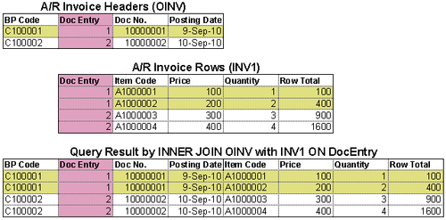
The previous example shows a real query about how an inner join works.
The query script is:
SELECT T0.CardCode as 'BP Code', T0.DocNum as 'Doc No.', T0.DocDate, T1.ItemCode, T1.Price as 'Price', T1.Quantity, T1.LineTotal
FROM dbo.OINV T0
INNER JOIN dbo.INV1 T1 ON T1.DocEntry = T0.DocEntry
Two tables, OINV (A/R invoice headers) and INV1 (A/R invoice rows), are joined by DocEntry columns. This DocEntry column is actually not included in the query result. It is only for illustration purposes for easier understanding. From the previous example, you can see how INNER JOIN works. For DocEntry 1 and 2, two rows each are formed by the query. The query result shows four lines in total.
You should avoid linking by lengthy text only columns. To match those columns, not only system performance becomes an issue, but also no ideal query results might be shown. In general, if the column length is over 30 characters, the link efficiency will be reduced dramatically.
Keep in mind, an inner join will effectively filter your query result by linking columns. If there are no common values between linked columns, those records are going to be dropped out. If you find that the query result does not meet your requirements, some other types of joins can be used instead.
Some may call OUTER JOIN a complex join. Actually, it may not be that complicated at all and is only a little bit more complicated than INNER JOIN. You do not need to worry about the complexity. When you find the true meaning of OUTER JOIN, it is similar and comparable with INNER JOIN.
There are three types of Outer Joins:
- Left Outer Join
- Right Outer Join
- Full Outer Join
We will examine each type as follows.
A LEFT OUTER JOIN is one of the most used outer joins in queries. Outer here is optional. It can be omitted so that you just need LEFT JOIN. There is no added benefit to using the full name of LEFT OUTER JOIN. Unless a query is automatically created, you should keep using only LEFT JOIN.
A LEFT JOIN clause syntax looks like the following:
SELECT T[0]|[1].column_name(s)
FROM table_name0 T0
LEFT JOIN table_name1 T1
ON T0.column_name=T1.column_name
In the previous syntax, the first table table_name0 T0 is the LEFT table, while table_name1 T1 is the right table. LEFT JOIN means all records in the left table will be returned, regardless of the right table linking condition. If the match cannot be found in T1 table, it simply returns Null value for any columns coming from T1 table.
A LEFT JOIN is very useful when you need to display all data records from one table but also want to know some secondary table data without restricting the query results. You will find more examples in the next chapter. If you are still not very clear about this LEFT JOIN clause, I hope the following example can help you:
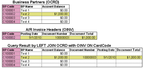
The previous example shows a real query about how LEFT JOIN works.
The query script is as follows:
SELECT T0.[CardCode], T0.[CardName], T0.[Balance], T1.[DocNum], T1.[DocDate], T1.[DocTotal]
FROM dbo.OCRD T0
LEFT JOIN dbo.OINV T1 ON T0.CardCode = T1.CardCode
WHERE T0.CardCode < 'C100005'
From the example, you can get a clear view. If you can only find one BP Code C100002 in the right table (OINV), you will get only one line with full information. All other lines will still show left table columns though.
One thing is important for a LEFT JOIN: do not use secondary Left Join if possible. Suppose you put more than one level of LEFT JOIN; the query result may become less clear.
A Right Outer Join is not used as often as a LEFT JOIN in a query. OUTER here is also optional. It can be omitted so that you just need RIGHT JOIN.
A RIGHT JOIN clause syntax looks like the following:
SELECT T[0]|[1].column_name(s)
FROM table_name0 T0
RIGHT JOIN table_name1 T1
ON T0.column_name=T1.column_name
In the previous syntax, the second table table_name1 T1 is the right table while table_name0 T0 is the left table. A RIGHT JOIN means all records in the right table will be returned, regardless of the left table linking condition. If the match cannot be found in T0 table, it simply returns Null value for any columns coming from the T0 table.
Most people would be more interested in the first table than the second table. That is why not so many people use this RIGHT JOIN. Here is an example for you:
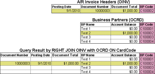
The query script is as follows:
SELECT T1.[DocNum], T1.[DocDate], T1.[DocTotal],T0.[CardName], T0.[Balance], T0.[CardCode]
FROM dbo.OINV T1
RIGHT JOIN dbo.OCRD T0 ON T0.CardCode = T1.CardCode
WHERE T0.CardCode < 'C100005'
Unless you are used to reading from right to left, I bet no user prefers this result instead of the LEFT JOIN.
A Full Outer Join syntax looks like the following:
SELECT T[0]|[1].column_name(s)
FROM table_name0 T0
FULL OUTER JOIN table_name1 T1
ON T0.column_name=T1.column_name
A Full Outer Join will return all rows from both tables, regardless of matching conditions. It is one of the most dangerous clauses for SELECT queries too. Try to avoid this kind of join wherever you have other options.
There is no example query for this kind of join because it may only be useful in very special cases.
For people who like to use a Full Outer Join, you should always check what alternatives you have. If only Full Outer Join can solve your issue, some big problems might be hidden. Check them out!
A Self-Join is a special join in which a table is joined to itself. Self-Joins are used to compare values in a column with other values in the same column in the same table. It can be used for certain special needs such as obtaining running counts or running totals in a SQL query. It is often used in subqueries.
To write a query that includes a Self-Join, select from the same table listed twice with different aliases, set up the comparison, or eliminate cases where a particular value would be equal to itself.
A Self-Join is mostly an INNER JOIN. However, it can also be an OUTER JOIN. It is all dependent on your needs.
To my knowledge, this join is only a particular type of INNER JOIN or OUTER JOIN. The classification makes it outstanding only because it is too special.
You will get some example queries of Self-Join in later chapters.
It is very clear that the WHERE clause is to define query conditions. By using the WHERE clause, you may extract only those records that fulfill a specified criterion.
The WHERE clause is optional. However, it is a good idea to make it mandatory for your own sake to keep your query results safer. When you create your query without a WHERE clause, all records will be retrieved no matter how big the table is. It is highly recommended that you put the WHERE clause for all of your query scripts before you test to run them. This can save you much more time if you just enter these few letters.
If the WHERE clause exists in a query, it always follows the FROM clause. Its syntax is as follows:
SELECT column_name(s)
FROM table_name(s)
WHERE [(]expression operator expression [and/or] [expression operator expression ][)]
In the previous syntax, expression stands for a column name, a constant, a function, a variable, or a subquery. An operator can be set from the following list:
|
Operator |
Description |
|---|---|
|
Equal | |
|
Not equal | |
|
Greater than | |
|
Less than | |
|
Not Greater than | |
|
Not Less than | |
|
Greater than or equal | |
|
Less than or equal | |
|
Between an inclusive range | |
|
Search for a pattern, used only for string | |
|
Test if a specified value matches any value in a subquery (or a list for IN operator only) |
If a column used in the WHERE clause is one of the character data types, the value must be enclosed in single quotes. In contrast, if the column used in the WHERE clause is of a numeric data type, the value should not be enclosed. The numeric values enclosed in quotes will always return 0.
To make the WHERE clause more efficient, it is better to avoid using Not Equal (<> /!=) wherever possible. Some of the other conditions with NOT also need to be used with care.
Five operators include >, <, =, >=, and <= symbols are very common for comparisons. They are not needed for the purpose of this book. Therefore they are omitted from the examples. Only three special comparisons will be discussed next.
A BETWEEN operator is to specify a range to test.
The syntax for a BETWEEN operator is:
Value1 [ NOT ] BETWEEN Value2 AND Value3
All arguments are discussed as follows:
- Value1 is the value to be tested in the range defined by Value2 and Value3.
- NOT specifies that the result of the predicate be negated. It is optional.
- Value1 is any valid value with the same data type as Values.
- Value3 is any valid value that is greater than Value2 with the same data type.
- AND is mandatory and acts as a placeholder that indicates Value1 should be within the range indicated by Value2 and Value3.
- This clause is equivalent to Value1 >= Value2 and Value1 <= Value3.
- When you use BETWEEN, it means that the start value and end value are included. If you need to specify an exclusive range, you have to use the greater than (>) and less than (<) operators instead.
There is a condition in the first query example in this chapter before discussing the statement:
WHERE t1.RefDate >= [%0] and t1.RefDate <= [%1]
Actually, it is equivalent to the following:
WHERE t1.RefDate BETWEEN [%0] and [%1]
The query result is exactly the same. I have chosen to use the longer expression only because the system prompt for the first one is better and clear.
IN or NOT IN is an operator to compare a value with an existing value list that has more than one value. You are allowed to have only one value in the list. However, that should be by equal operator. It is not logical to define only one value in the list. An IN operator can be used to determine whether a specified value matches or does not match any values in a list. The list can be a result of a subquery. This subquery must have only one column to return. In order for two sides to be comparable, both sides must have matched data types.
This operator is similar to the OR condition but is much shorter. With the OR condition, you not only have to repeat the similar conditions one by one, but you also need parentheses if there are other co-existing conditions.
In the list to be compared, duplicate values are allowed. You do not need to specify the DISTINCT keyword if the same values are the same. After all, you are comparing the left side value to the right side value list. The result will be the same no matter how many times the same values present in the list are compared with.
Any null values returned by a subquery or a list that are to be compared using IN or NOT IN will return UNKNOWN. It can produce unexpected results. Get rid of the Null value for the list wherever possible.
EXISTS or NOT EXISTS is also an operator to compare a value with a list. The list is only a result of a subquery. This subquery can have more than one column to return. In order for two sides to be comparable, both sides must have matched data types.
IN and EXISTS are almost the same, only that IN allows both fixed list and subquery. The only other exception is the way they treat Null values. If the subquery contains Null value, EXISTS will perform better than IN. This is because EXISTS only cares if the value exists in the query result. It doesn't care if there is Null value or not.
The bottom line is: whenever using these operators, predict if you may get Null values. Choose a proper one based on the prediction.
A LIKE operator allows you to do a search based on a pattern rather than specifying exactly what is desired (as in IN) or spell out a range (as in BETWEEN). LIKE determines whether a value to be tested matches a specified pattern. A pattern can include wildcard characters. During this matching, wildcard characters play flexible roles to allow partly unmatched values to go through.
Using wildcard characters makes the LIKE operator more flexible than using the = or != string comparison operators. In case any one of the values is not of the character string data type, the SQL Server Database Engine converts them to character string data type if possible.
A LIKE operator syntax is as follows:
Value [ NOT ] LIKE Pattern
Two arguments are as follows:
|
Description | |
|---|---|
|
Any string with zero or more characters | |
|
Any single character | |
|
Any single character within the specified range ([a-d]) or set ([abcd]) | |
|
Any single character not within the specified range ([^x-z]) or set ([^xyz]) |
Most of the LIKE operators include % and/or _ wildcard characters. % can be put in the front, in the middle, or at the end. If you can find a certain condition such as A LIKE 'xy%' instead of A LIKE '%xy', the query result would be faster.
Although NOT is an optional keyword for LIKE, you should try to avoid it in any way possible. It is not an effective way to compare a value with any patterns.
A GROUP BY clause is very useful if you need to aggregate your data based on certain columns. It is optional and must follow the FROM and WHERE clauses.
If you remember the first query before discussing statements, you have:
GROUP BY T0.ShortName
GROUP BY specifies T0.ShortName i.e. Business Partner column would be the base for summarizing debit and credit amounts for each Business Partner.
Whenever you use the GROUP BY clause, it is mandatory to include all your columns under this clause unless they are aggregated columns.
The following example shows a simple query:

The query script is simple:
SELECT T0.CardCode AS 'BP Code', T0.CardName AS 'BP Named', SUM(T0.DocTotal) AS 'Total'
FROM dbo.OINV T0
WHERE T0.CardCode < 'C100003'
GROUP BY T0.CardCode, T0.CardName
In the previous example, neither the DocNum nor the DocTotal columns can be included in the query. Otherwise, the group will not work for each customer.
A HAVING clause is normally used with a GROUP BY clause. This clause is optional. It is equivalent to a WHERE clause under the main query body. It specifies that a SELECT statement should only return rows where aggregate values meet the specified conditions. This clause was added to the SQL language after the main clause had already been defined because the WHERE keyword could not be used with aggregate functions.
If you remember the first query before discussing, you have:
HAVING SUM(ISNULL(T0.Debit,0) - ISNULL(T0.Credit,0)) > 0
It can be found under the GROUP BY clause in the query. This means the query result will only include those records if the aggregate summary function's result of T0.Debit minus T0.Credit is greater than zero. In case there are Null values, they will be replaced with zero from all occurrences before summary operation.
An ORDER BY clause is very simple when you need to sort your query result based on certain columns. This clause is always the last clause to be used in the query. If you have UNION or UNION ALL to combine more than one query, this clause may only be added to the end of the entire query.
There are two types of orders: One is ascending and the other is descending. Descending can be abbreviated to DESC in the end. Ascending can be abbreviated to ASC. If DESC is not included, the default ORDER BY will be ascending. Since ascending is the default order, it is usually omitted from the query.
An ORDER BY clause can have more than one column. The rule for query result is: the order first applies to the first column in the left. Then will be the second column, the third column, and so on.
Remember, not all types of columns are orderable. Some image columns, memo columns, etc. cannot be ordered.
If you remember the first query before the discussion statement, the last statement is as follows:
ORDER BY SUM(ISNULL(T0.Debit,0) - ISNULL(T0.Credit,0)) DESC
It means the query result will be ordered by descending order according to the summary of T0.Debit minus T0.Credit. If there are Null values, they will be replaced with zero for all occurrences.
The UNION clause combines the results of two or more SQL queries into one query result set. To use this clause, the number and order of columns from those queries must be the same with compatible data types. Any duplicate records are automatically removed by the UNION clause. It works like DISTINCT.
One thing you need to be aware of: UNION results do not care about the order of the rows. Rows from the first query may appear before, after, or mixed with rows from the following one. If you need a specific order, the ORDER BY clause must be used.
The UNION ALL clause is almost the same as the UNION clause, except it allows duplicated records.
UNION ALL may be much faster than plain UNION due to fewer checks in the query process. Whenever duplication is not a concern, or duplication is needed, UNION ALL should be used first.
A UNION or UNION ALL query is usually longer than a normal query because it is at least double the lines of query scripts. The example query that includes this clause will be shown in later chapters.
SELECT—first statement to retrieve data
It is quite obvious from the meaning of the word that SELECT is used to display or retrieve data from certain data sources.
The SELECT statement is used to return data from a set of values or database tables.
The result is stored in a result table, called the result-set.
SELECT is one of the most commonly used Data Manipulation Language (DML) commands. It seems very simple. However, something important needs to be explained for this statement:
- The scope of the value that can be retrieved
- The numbers of columns to be included
- Column name descriptions
- Keywords followed to this statement
Here is a return value list that SELECT can be used for:
- A single value
- A group of values
- Return a single database table column
- Return a group of database table columns
- Return complete database table columns
- Used in a subquery
The simplest SELECT query would be just to get a constant or text without any additional statements. An example would be:
SELECT 'YES' AS 'Yes/No' or
SELECT 10 AS 'No.'
These queries will display Yes or 10 in one column when executed.
You may also use this statement to get a group of values. For example:
SELECT 'YES' AS 'Yes/No', 10 AS 'No.', 'This is an example' AS 'Content'
This query will display Yes, 10, This is an example in three columns named Yes/No, No., and Content when you execute it.
Some special uses of this statement to display a single value or group of values will be discussed in other chapters when we introduce more specific topics.
Please note the comma used above. Following the SELECT statement, each comma will define a new column to be displayed.
Tip
Do not forget to delete the last comma in a SELECT statement. This simple mistake is one of the most frequent problems for a query. It is mainly due to the fact that we are often used to copying columns in our queries, which include the comma, and forget to remove the last one before testing the query.
Similar to the single value SELECT, we can use it for a database table column. Here is an example:
SELECT CompnyName
FROM OADM
This simple example will retrieve your company name from table OADM.
The formal query should be this:
SELECT T0.CompnyName
FROM dbo.OADM T0
It is an important step to include Alias (T0) and Database Owner (dbo) for the table in the query. It will ensure the query's consistency and efficiency. This topic will be discussed in the FROM clause in more detail.
There is no big difference with the previous example. We can use the same principle to select multiple database table columns. For instance:
SELECT CompnyName, CompnyAddr, Country, Phone1
FROM OADM
This example will retrieve not only your company name, but also your company's address, country, and phone number from table OADM.
The formal query should be as follows:
SELECT T0.CompnyName, T0.CompnyAddr, T0.Country, T0.Phone1 FROM dbo.OADM T0
This is the simplest query to return all column values from table. That is:
SELECT *
FROM OADM
This example will retrieve every single column from table OADM. There is no need to assign alias to the query because this kind of query is usually a one-time only query. Here, * is a wildcard that represents everything in the table.
Note
Be careful when running SELECT * from a huge table such as JDT1. It may affect your system's performance! If you are not sure about the table size, it is safer for you to always include the WHERE clause with reasonable restrictions. Or you can run SELECT COUNT(*) FROM the table you want to query first. If the number is high, do not run it without a condition clause.
How many columns are suitable for a query? I don't think there are any standard answers. In my experience, I can only suggest to you: the shorter, the better.
Some people have the tendency to include all information in one report. This kind of request may even come from certain executives of the company's management.
One simple test would be a fair criterion. Can you fit the query result within the query result window? If you can, great; that would be a proper number of columns. If not, then I would strongly suggest you double check every column to see if you can cut one or more of them out.
If it is a query for alert, it needs even more special care. The column numbers in any alert queries have to be trimmed to the minimum. Otherwise, you may only get part of the result due to the query result size limitation. You will get more explanation for this issue in the chapter for alert queries.
If you are requested to create super long and wide queries, explain the consequences to the person in charge. Sometimes, they can change their mind depending on the way you communicate with them. In my experience, if a print out report cannot be handled within the width of a page, it might make the report difficult to read. Show the result to a non-technical person. It is easily understandable when you can bring the first hand output to the report readers.
Column names usually come directly from column descriptions, if you have not reassigned them in the query. You can, however, change them to make the query result more useful for special cases. Some people use this method to translate the description into their local language. Some people use it to make the column description more clear.
For some of the value-only columns or formula columns it is mandatory to assign descriptions, otherwise the column headings would be empty. This not only looks unprofessional, but you will also have no way to export the query results to Excel for those columns without the description.
You can use single or double quotation marks for the description. If the description has only one word, you can even omit the quotation mark. The syntax is shown next:
[ColumnName] AS 'Column Description Here'
You can omit AS, so that you just keep [ColumnName] 'Description Here'. However, whenever possible, you should keep the AS to make the query script more consistent.
A DISTINCT clause is used for getting rid of duplicated records to return only distinct (different) values.
The syntax of this clause is:
SELECT DISTINCT column_name(s)
FROM table_name(s)
column_name and table_name are self explanatory. They represent column name and table name respectively. There will be no additional denotation for these two clauses in this book. A DISTINCT clause is always the first one after the SELECT statement. It is optional. When you specify Distinct in the query, it will not allow any identical rows in the query result. All lines are unique from each other.
Some users claim this clause may still allow duplicate rows. This can never be true. The fact is: although most of the values are the same between two lines, the query results always include at least one column, which contains the different values. Those columns have to be taken out in order to benefit from this clause. You cannot get both the DISTINCT working and some columns which have different values within the scope you selected.
A TOP clause is used to specify the maximum number of records to return in a query result-set. It is usually used together with the Order By clause at the end of the query.
The syntax of the clause is as follows:
SELECT TOP (number)|percent[with ties] column_name(s)
FROM table_name(s)
The query result can be the top 10 sales orders, for example. In this case, descending order must be used for the document amounts. Or you may get the top 20 percent purchase invoices, if you specify the TOP by percentage. When you use percentage, you need to write
20 percent instead of 20% after SELECT TOP.
The WITH TIES option specifies the additional rows that need to be returned from the base result set with the same value in the ORDER BY columns appearing at the end of the TOP n (PERCENT) rows. TOP...WITH TIES can be specified only if an ORDER BY clause is specified.
Microsoft suggests SELECT TOP (n) with parentheses. It is better to follow the suggestion to be safe for the query results.
It is very clear that FROM means where to find the data. A FROM clause is actually not a standalone statement since it must be used with SELECT. Most queries need this clause because to only assign a fixed value or a group of values would not be very useful. However, this is one of the most often misused parts of SQL queries. More discussion is needed on this clause.
A FROM clause can be followed by the data sources mentioned next:
Tip
If you have read through Chapter 1, SAP Business One Query Users and Query Basic, you should understand the concept of Table and Table Relationships. If you directly jumped here bypassing that previous chapter, you may need to go back to check.
This is the simplest query including a FROM statement. A simple example:
SELECT Code, Name, Remarks FROM OUDP
This will only touch one table—OUDP. This table is for a department. You can get the Department Code, Department Name, and the Description from the query result.
The better format would be:
SELECT T0.Code, T0.Name, T0.Remarks FROM dbo.OUDP T0
Now, it is time to explain why those additional T0 and dbo are necessary here.
Actually, it may not make any difference if we only deal with this particular query and this query is only run by one user. However, that is not generally true. In most cases, we often have more than one table and more than one user to run the same query.
T0 here stands for an Alias of OUDP table. It is the standard convention and most frequently used alias. T means table. 0 is a sequence number. You can have T0, T1, T2, …until Tn. If you have 10 tables in the query, n would be equal to 9 for alias. This naming convention is convenient to use. You just need to name them in sequential numbers.
The syntax for table alias looks like this:
SELECT alias_table_name.column_name
FROM table_name [AS] alias_table_name
An alias table name can be anything, but usually it is the shortest possible one.
If a query is not created by query tools, it is not mandatory for alias to take the Tn sequence. You may just use A, B, C, …… to have one letter shorter than the standard way, or make them easier to remember. However, it is advisable that you follow the norm. It can save you time for maintaining your query in the long run.
The function for alias is mainly for saving resources. If no alias is defined, you have to enter the full table names for every single column in the query. Be careful when you are using alias; you should use alias exclusively throughout your query. You are not allowed to mix them with the actual table name. In other words, you may only use alias or the actual table name, but you are not allowed to use them both in the same query.
The other added word dbo means Database Owner. This is a special database user. This user has implied permissions to perform all activities in the database. All tables of SAP Business One have the owner of dbo. It is useful to add dbo in front of a table name when you have more than one user running the query, but this is beyond the scope of the book. I will try to use the simplest method to give you a rough idea.
Query running needs an execution plan. A query execution plan (or query plan) outlines how the SQL Server query optimizer (query optimizer is too complicated to explain here, you just need to know it is a tool built into SQL server) actually ran (or will run) a specific query. There are typically a large number of alternate ways to execute a given query, with widely varying performance. When a query is submitted to the database, the query optimizer evaluates some of the different, correct possible plans for executing the query and returns what it considers the best alternative. This information is very valuable when it comes to finding out why a specific query is running slowly.
The hard fact is: no one can control this plan manually at runtime. Once a plan is created, it is reusable for the same user to run the query. If you are not entering dbo in front of the table name, the query will check every user who runs the query. A new plan may be added for every new user because the owner is not included in the query body. That might cause too much unnecessary burden to the database.
This is the category that most queries will be included in. One example may not be enough to show this clearly. You have two query examples to show. The first one is as follows:
SELECT Distinct T0.[DocNum], T1.DocNum, T0.[DocType], T0.[CardCode], T0.[CardName], T0.[UserSign], T0.[UserSign2], T1.[UserSign], T1.[UserSign2]
FROM dbo.ADOC T0
INNER JOIN dbo.ORIN T1 ON T0.DocNum = T1.DocNum
WHERE T0.[ObjType] = '14' AND T0.[UserSign2] != T1.[UserSign2]
This query links ADOC (Document History) and ORIN (Credit Memo Headers) tables to show the credit memo document number, document type, user information, and the change log user code for the credit memo. A detailed explanation can be found in the next chapter.
The second query example is as follows:
SELECT T1.CardCode as "CustCode", T1.CardName as "CustName", T2.SlpName, T1.DocNum "Incoming#", T1.DocDate, T1.DocTotal as "Payment Total", T4.DocNum as "Invoice#", T3.SumApplied as "Applied Total"
FROM dbo.OCRD T0
INNER JOIN dbo.ORCT T1 ON T0.CardCode = T1.CardCode
LEFT JOIN dbo.OSLP T2 ON T0.SlpCode = T2.SlpCode
INNER JOIN dbo.RCT2 T3 ON T3.DocNum = T1.DocNum
INNER JOIN dbo.OINV T4 ON T4.DocEntry = T3.DocENtry AND T3.InvType = '13'
WHERE T1.DocDate >= [%0] AND T1.DocDate <= [%1]
ORDER by T1.DocDate
This query links five tables OCRD (Business Partners), ORCT (Incoming Payment Headers), RCT2 (Incoming Payments—Invoices), OSLP (Sales Employees), and OINV (Invoice Headers) together. It shows customers' payment with invoice details. Again, the business case explanation is available in the next chapter.
Among the five links in the query, there are two different kinds of links. One is INNER JOIN. The other is LEFT JOIN; more explanation of these joins can be found later in the chapter.
When you link tables together, SQL Server just treats them as a view, or it acts as one big table. However, there is another way to add your tables into the query without linking them first. The syntax is similar to comma delimited columns. You simply need to enter a comma in between tables. In this case, table linking has to be done under the WHERE conditions.
Technically, the way of linking tables without joining is the most ideal method because you can get the minimum records out with the least database operations, if you are very good at database structure. However, like the difference between manual and automatic cameras, most people prefer automatic cameras because it is very convenient, especially if you do not have extensive training or extraordinary experience, and the ideal manual control may not help you get a better picture!
I always refuse to create queries without joining the tables first. Comma-separated table query is too dangerous. If you have the wrong conditions defined in the WHERE clause, you may end up with countless loops. In the worst case scenario, it may lock your system up. On the contrary, if you link all tables together, the worst case scenario would be no results because of a bad link or bad conditions.
In other words, if you want to add all tables' linking conditions under the WHERE clause, you are giving yourself an unnecessary burden in making sure they are correct. Those verifications have to be done manually.
Whenever possible, you are better to avoid using comma separated table queries. In most cases, it may use more resources and put you at a higher risk of system instability.
You have learned the FROM statement. With this statement, you know that more than one table can be put into one query.
In most cases, those additional tables should be linked together. The reason we need to link tables before the WHERE clause has been discussed in the previous paragraph. To link those extra tables, JOIN is used to combine rows from multiple tables.
A join is performed whenever two or more tables are listed in the FROM clause of a SQL statement without using a comma to separate them. Joined tables must include at least one common column in both tables that contain comparable data. Column names across tables don't have to be the same. But if we have the same name columns to join with correct relation, use them first.
There are different types of JOIN statements to be discussed, listed as follows:
- Inner join
- Outer joins
- Self-join
One of the special join types is omitted from the list. This is called the Cross Join. This type of join can list all possible combinations of your linked tables. You may end up with 90,000 lines of huge output even if you have only 300 records in each table. I have no idea who can benefit from this Cross Join. They must be very special.
First, let's look at the most commonly used one.
An INNER JOIN is also called a Simple Join. It is the simplest table join. INNER JOIN is the default link type to join tables. You may even omit INNER to leave only JOIN. When you see JOIN without any words in front, it means INNER JOIN. In order to distinguish other types of JOIN, omission is not encouraged unless your query length is an issue that requires you to reduce your query to the minimum size.
An INNER JOIN syntax looks like the following:
SELECT T[0]|[1].column_name(s)
FROM table_name0 T0
INNER JOIN table_name1 T1
ON T0.column_name=T1.column_name
In an INNER JOIN statement, the link is defined by the keyword ON with common columns from each table to retrieve the matching records from those tables. To link two or more tables correctly, the linking columns are very important. INNER JOIN will select all rows from linked tables as long as there is a match between the columns you are matching on. If you forget the keyword ON in the joined table list, you will get an error message right away when you try to run the query.
The best way to link tables is by using the Key Columns such as the primary key or the foreign key. That is because Key Columns are usually indexed. That makes links easier and faster. In case there is no such columns' pair to link, care must be taken to select the best efficient common columns between tables. When you have more than one way to link, you can consider the shorter columns first.
The previous example shows a real query about how an inner join works.
The query script is:
SELECT T0.CardCode as 'BP Code', T0.DocNum as 'Doc No.', T0.DocDate, T1.ItemCode, T1.Price as 'Price', T1.Quantity, T1.LineTotal
FROM dbo.OINV T0
INNER JOIN dbo.INV1 T1 ON T1.DocEntry = T0.DocEntry
Two tables, OINV (A/R invoice headers) and INV1 (A/R invoice rows), are joined by DocEntry columns. This DocEntry column is actually not included in the query result. It is only for illustration purposes for easier understanding. From the previous example, you can see how INNER JOIN works. For DocEntry 1 and 2, two rows each are formed by the query. The query result shows four lines in total.
You should avoid linking by lengthy text only columns. To match those columns, not only system performance becomes an issue, but also no ideal query results might be shown. In general, if the column length is over 30 characters, the link efficiency will be reduced dramatically.
Keep in mind, an inner join will effectively filter your query result by linking columns. If there are no common values between linked columns, those records are going to be dropped out. If you find that the query result does not meet your requirements, some other types of joins can be used instead.
Some may call OUTER JOIN a complex join. Actually, it may not be that complicated at all and is only a little bit more complicated than INNER JOIN. You do not need to worry about the complexity. When you find the true meaning of OUTER JOIN, it is similar and comparable with INNER JOIN.
There are three types of Outer Joins:
- Left Outer Join
- Right Outer Join
- Full Outer Join
We will examine each type as follows.
A LEFT OUTER JOIN is one of the most used outer joins in queries. Outer here is optional. It can be omitted so that you just need LEFT JOIN. There is no added benefit to using the full name of LEFT OUTER JOIN. Unless a query is automatically created, you should keep using only LEFT JOIN.
A LEFT JOIN clause syntax looks like the following:
SELECT T[0]|[1].column_name(s)
FROM table_name0 T0
LEFT JOIN table_name1 T1
ON T0.column_name=T1.column_name
In the previous syntax, the first table table_name0 T0 is the LEFT table, while table_name1 T1 is the right table. LEFT JOIN means all records in the left table will be returned, regardless of the right table linking condition. If the match cannot be found in T1 table, it simply returns Null value for any columns coming from T1 table.
A LEFT JOIN is very useful when you need to display all data records from one table but also want to know some secondary table data without restricting the query results. You will find more examples in the next chapter. If you are still not very clear about this LEFT JOIN clause, I hope the following example can help you:
The previous example shows a real query about how LEFT JOIN works.
The query script is as follows:
SELECT T0.[CardCode], T0.[CardName], T0.[Balance], T1.[DocNum], T1.[DocDate], T1.[DocTotal]
FROM dbo.OCRD T0
LEFT JOIN dbo.OINV T1 ON T0.CardCode = T1.CardCode
WHERE T0.CardCode < 'C100005'
From the example, you can get a clear view. If you can only find one BP Code C100002 in the right table (OINV), you will get only one line with full information. All other lines will still show left table columns though.
One thing is important for a LEFT JOIN: do not use secondary Left Join if possible. Suppose you put more than one level of LEFT JOIN; the query result may become less clear.
A Right Outer Join is not used as often as a LEFT JOIN in a query. OUTER here is also optional. It can be omitted so that you just need RIGHT JOIN.
A RIGHT JOIN clause syntax looks like the following:
SELECT T[0]|[1].column_name(s)
FROM table_name0 T0
RIGHT JOIN table_name1 T1
ON T0.column_name=T1.column_name
In the previous syntax, the second table table_name1 T1 is the right table while table_name0 T0 is the left table. A RIGHT JOIN means all records in the right table will be returned, regardless of the left table linking condition. If the match cannot be found in T0 table, it simply returns Null value for any columns coming from the T0 table.
Most people would be more interested in the first table than the second table. That is why not so many people use this RIGHT JOIN. Here is an example for you:
The query script is as follows:
SELECT T1.[DocNum], T1.[DocDate], T1.[DocTotal],T0.[CardName], T0.[Balance], T0.[CardCode]
FROM dbo.OINV T1
RIGHT JOIN dbo.OCRD T0 ON T0.CardCode = T1.CardCode
WHERE T0.CardCode < 'C100005'
Unless you are used to reading from right to left, I bet no user prefers this result instead of the LEFT JOIN.
A Full Outer Join syntax looks like the following:
SELECT T[0]|[1].column_name(s)
FROM table_name0 T0
FULL OUTER JOIN table_name1 T1
ON T0.column_name=T1.column_name
A Full Outer Join will return all rows from both tables, regardless of matching conditions. It is one of the most dangerous clauses for SELECT queries too. Try to avoid this kind of join wherever you have other options.
There is no example query for this kind of join because it may only be useful in very special cases.
For people who like to use a Full Outer Join, you should always check what alternatives you have. If only Full Outer Join can solve your issue, some big problems might be hidden. Check them out!
A Self-Join is a special join in which a table is joined to itself. Self-Joins are used to compare values in a column with other values in the same column in the same table. It can be used for certain special needs such as obtaining running counts or running totals in a SQL query. It is often used in subqueries.
To write a query that includes a Self-Join, select from the same table listed twice with different aliases, set up the comparison, or eliminate cases where a particular value would be equal to itself.
A Self-Join is mostly an INNER JOIN. However, it can also be an OUTER JOIN. It is all dependent on your needs.
To my knowledge, this join is only a particular type of INNER JOIN or OUTER JOIN. The classification makes it outstanding only because it is too special.
You will get some example queries of Self-Join in later chapters.
It is very clear that the WHERE clause is to define query conditions. By using the WHERE clause, you may extract only those records that fulfill a specified criterion.
The WHERE clause is optional. However, it is a good idea to make it mandatory for your own sake to keep your query results safer. When you create your query without a WHERE clause, all records will be retrieved no matter how big the table is. It is highly recommended that you put the WHERE clause for all of your query scripts before you test to run them. This can save you much more time if you just enter these few letters.
If the WHERE clause exists in a query, it always follows the FROM clause. Its syntax is as follows:
SELECT column_name(s)
FROM table_name(s)
WHERE [(]expression operator expression [and/or] [expression operator expression ][)]
In the previous syntax, expression stands for a column name, a constant, a function, a variable, or a subquery. An operator can be set from the following list:
|
Operator |
Description |
|---|---|
|
Equal | |
|
Not equal | |
|
Greater than | |
|
Less than | |
|
Not Greater than | |
|
Not Less than | |
|
Greater than or equal | |
|
Less than or equal | |
|
Between an inclusive range | |
|
Search for a pattern, used only for string | |
|
Test if a specified value matches any value in a subquery (or a list for IN operator only) |
If a column used in the WHERE clause is one of the character data types, the value must be enclosed in single quotes. In contrast, if the column used in the WHERE clause is of a numeric data type, the value should not be enclosed. The numeric values enclosed in quotes will always return 0.
To make the WHERE clause more efficient, it is better to avoid using Not Equal (<> /!=) wherever possible. Some of the other conditions with NOT also need to be used with care.
Five operators include >, <, =, >=, and <= symbols are very common for comparisons. They are not needed for the purpose of this book. Therefore they are omitted from the examples. Only three special comparisons will be discussed next.
A BETWEEN operator is to specify a range to test.
The syntax for a BETWEEN operator is:
Value1 [ NOT ] BETWEEN Value2 AND Value3
All arguments are discussed as follows:
- Value1 is the value to be tested in the range defined by Value2 and Value3.
- NOT specifies that the result of the predicate be negated. It is optional.
- Value1 is any valid value with the same data type as Values.
- Value3 is any valid value that is greater than Value2 with the same data type.
- AND is mandatory and acts as a placeholder that indicates Value1 should be within the range indicated by Value2 and Value3.
- This clause is equivalent to Value1 >= Value2 and Value1 <= Value3.
- When you use BETWEEN, it means that the start value and end value are included. If you need to specify an exclusive range, you have to use the greater than (>) and less than (<) operators instead.
There is a condition in the first query example in this chapter before discussing the statement:
WHERE t1.RefDate >= [%0] and t1.RefDate <= [%1]
Actually, it is equivalent to the following:
WHERE t1.RefDate BETWEEN [%0] and [%1]
The query result is exactly the same. I have chosen to use the longer expression only because the system prompt for the first one is better and clear.
IN or NOT IN is an operator to compare a value with an existing value list that has more than one value. You are allowed to have only one value in the list. However, that should be by equal operator. It is not logical to define only one value in the list. An IN operator can be used to determine whether a specified value matches or does not match any values in a list. The list can be a result of a subquery. This subquery must have only one column to return. In order for two sides to be comparable, both sides must have matched data types.
This operator is similar to the OR condition but is much shorter. With the OR condition, you not only have to repeat the similar conditions one by one, but you also need parentheses if there are other co-existing conditions.
In the list to be compared, duplicate values are allowed. You do not need to specify the DISTINCT keyword if the same values are the same. After all, you are comparing the left side value to the right side value list. The result will be the same no matter how many times the same values present in the list are compared with.
Any null values returned by a subquery or a list that are to be compared using IN or NOT IN will return UNKNOWN. It can produce unexpected results. Get rid of the Null value for the list wherever possible.
EXISTS or NOT EXISTS is also an operator to compare a value with a list. The list is only a result of a subquery. This subquery can have more than one column to return. In order for two sides to be comparable, both sides must have matched data types.
IN and EXISTS are almost the same, only that IN allows both fixed list and subquery. The only other exception is the way they treat Null values. If the subquery contains Null value, EXISTS will perform better than IN. This is because EXISTS only cares if the value exists in the query result. It doesn't care if there is Null value or not.
The bottom line is: whenever using these operators, predict if you may get Null values. Choose a proper one based on the prediction.
A LIKE operator allows you to do a search based on a pattern rather than specifying exactly what is desired (as in IN) or spell out a range (as in BETWEEN). LIKE determines whether a value to be tested matches a specified pattern. A pattern can include wildcard characters. During this matching, wildcard characters play flexible roles to allow partly unmatched values to go through.
Using wildcard characters makes the LIKE operator more flexible than using the = or != string comparison operators. In case any one of the values is not of the character string data type, the SQL Server Database Engine converts them to character string data type if possible.
A LIKE operator syntax is as follows:
Value [ NOT ] LIKE Pattern
Two arguments are as follows:
|
Description | |
|---|---|
|
Any string with zero or more characters | |
|
Any single character | |
|
Any single character within the specified range ([a-d]) or set ([abcd]) | |
|
Any single character not within the specified range ([^x-z]) or set ([^xyz]) |
Most of the LIKE operators include % and/or _ wildcard characters. % can be put in the front, in the middle, or at the end. If you can find a certain condition such as A LIKE 'xy%' instead of A LIKE '%xy', the query result would be faster.
Although NOT is an optional keyword for LIKE, you should try to avoid it in any way possible. It is not an effective way to compare a value with any patterns.
A GROUP BY clause is very useful if you need to aggregate your data based on certain columns. It is optional and must follow the FROM and WHERE clauses.
If you remember the first query before discussing statements, you have:
GROUP BY T0.ShortName
GROUP BY specifies T0.ShortName i.e. Business Partner column would be the base for summarizing debit and credit amounts for each Business Partner.
Whenever you use the GROUP BY clause, it is mandatory to include all your columns under this clause unless they are aggregated columns.
The following example shows a simple query:
The query script is simple:
SELECT T0.CardCode AS 'BP Code', T0.CardName AS 'BP Named', SUM(T0.DocTotal) AS 'Total'
FROM dbo.OINV T0
WHERE T0.CardCode < 'C100003'
GROUP BY T0.CardCode, T0.CardName
In the previous example, neither the DocNum nor the DocTotal columns can be included in the query. Otherwise, the group will not work for each customer.
A HAVING clause is normally used with a GROUP BY clause. This clause is optional. It is equivalent to a WHERE clause under the main query body. It specifies that a SELECT statement should only return rows where aggregate values meet the specified conditions. This clause was added to the SQL language after the main clause had already been defined because the WHERE keyword could not be used with aggregate functions.
If you remember the first query before discussing, you have:
HAVING SUM(ISNULL(T0.Debit,0) - ISNULL(T0.Credit,0)) > 0
It can be found under the GROUP BY clause in the query. This means the query result will only include those records if the aggregate summary function's result of T0.Debit minus T0.Credit is greater than zero. In case there are Null values, they will be replaced with zero from all occurrences before summary operation.
An ORDER BY clause is very simple when you need to sort your query result based on certain columns. This clause is always the last clause to be used in the query. If you have UNION or UNION ALL to combine more than one query, this clause may only be added to the end of the entire query.
There are two types of orders: One is ascending and the other is descending. Descending can be abbreviated to DESC in the end. Ascending can be abbreviated to ASC. If DESC is not included, the default ORDER BY will be ascending. Since ascending is the default order, it is usually omitted from the query.
An ORDER BY clause can have more than one column. The rule for query result is: the order first applies to the first column in the left. Then will be the second column, the third column, and so on.
Remember, not all types of columns are orderable. Some image columns, memo columns, etc. cannot be ordered.
If you remember the first query before the discussion statement, the last statement is as follows:
ORDER BY SUM(ISNULL(T0.Debit,0) - ISNULL(T0.Credit,0)) DESC
It means the query result will be ordered by descending order according to the summary of T0.Debit minus T0.Credit. If there are Null values, they will be replaced with zero for all occurrences.
The UNION clause combines the results of two or more SQL queries into one query result set. To use this clause, the number and order of columns from those queries must be the same with compatible data types. Any duplicate records are automatically removed by the UNION clause. It works like DISTINCT.
One thing you need to be aware of: UNION results do not care about the order of the rows. Rows from the first query may appear before, after, or mixed with rows from the following one. If you need a specific order, the ORDER BY clause must be used.
The UNION ALL clause is almost the same as the UNION clause, except it allows duplicated records.
UNION ALL may be much faster than plain UNION due to fewer checks in the query process. Whenever duplication is not a concern, or duplication is needed, UNION ALL should be used first.
A UNION or UNION ALL query is usually longer than a normal query because it is at least double the lines of query scripts. The example query that includes this clause will be shown in later chapters.
The scope of the value that can be retrieved
Here is a return value list that SELECT can be used for:
- A single value
- A group of values
- Return a single database table column
- Return a group of database table columns
- Return complete database table columns
- Used in a subquery
The simplest SELECT query would be just to get a constant or text without any additional statements. An example would be:
SELECT 'YES' AS 'Yes/No' or
SELECT 10 AS 'No.'
These queries will display Yes or 10 in one column when executed.
You may also use this statement to get a group of values. For example:
SELECT 'YES' AS 'Yes/No', 10 AS 'No.', 'This is an example' AS 'Content'
This query will display Yes, 10, This is an example in three columns named Yes/No, No., and Content when you execute it.
Some special uses of this statement to display a single value or group of values will be discussed in other chapters when we introduce more specific topics.
Please note the comma used above. Following the SELECT statement, each comma will define a new column to be displayed.
Tip
Do not forget to delete the last comma in a SELECT statement. This simple mistake is one of the most frequent problems for a query. It is mainly due to the fact that we are often used to copying columns in our queries, which include the comma, and forget to remove the last one before testing the query.
Similar to the single value SELECT, we can use it for a database table column. Here is an example:
SELECT CompnyName
FROM OADM
This simple example will retrieve your company name from table OADM.
The formal query should be this:
SELECT T0.CompnyName
FROM dbo.OADM T0
It is an important step to include Alias (T0) and Database Owner (dbo) for the table in the query. It will ensure the query's consistency and efficiency. This topic will be discussed in the FROM clause in more detail.
There is no big difference with the previous example. We can use the same principle to select multiple database table columns. For instance:
SELECT CompnyName, CompnyAddr, Country, Phone1
FROM OADM
This example will retrieve not only your company name, but also your company's address, country, and phone number from table OADM.
The formal query should be as follows:
SELECT T0.CompnyName, T0.CompnyAddr, T0.Country, T0.Phone1 FROM dbo.OADM T0
This is the simplest query to return all column values from table. That is:
SELECT *
FROM OADM
This example will retrieve every single column from table OADM. There is no need to assign alias to the query because this kind of query is usually a one-time only query. Here, * is a wildcard that represents everything in the table.
Note
Be careful when running SELECT * from a huge table such as JDT1. It may affect your system's performance! If you are not sure about the table size, it is safer for you to always include the WHERE clause with reasonable restrictions. Or you can run SELECT COUNT(*) FROM the table you want to query first. If the number is high, do not run it without a condition clause.
How many columns are suitable for a query? I don't think there are any standard answers. In my experience, I can only suggest to you: the shorter, the better.
Some people have the tendency to include all information in one report. This kind of request may even come from certain executives of the company's management.
One simple test would be a fair criterion. Can you fit the query result within the query result window? If you can, great; that would be a proper number of columns. If not, then I would strongly suggest you double check every column to see if you can cut one or more of them out.
If it is a query for alert, it needs even more special care. The column numbers in any alert queries have to be trimmed to the minimum. Otherwise, you may only get part of the result due to the query result size limitation. You will get more explanation for this issue in the chapter for alert queries.
If you are requested to create super long and wide queries, explain the consequences to the person in charge. Sometimes, they can change their mind depending on the way you communicate with them. In my experience, if a print out report cannot be handled within the width of a page, it might make the report difficult to read. Show the result to a non-technical person. It is easily understandable when you can bring the first hand output to the report readers.
Column names usually come directly from column descriptions, if you have not reassigned them in the query. You can, however, change them to make the query result more useful for special cases. Some people use this method to translate the description into their local language. Some people use it to make the column description more clear.
For some of the value-only columns or formula columns it is mandatory to assign descriptions, otherwise the column headings would be empty. This not only looks unprofessional, but you will also have no way to export the query results to Excel for those columns without the description.
You can use single or double quotation marks for the description. If the description has only one word, you can even omit the quotation mark. The syntax is shown next:
[ColumnName] AS 'Column Description Here'
You can omit AS, so that you just keep [ColumnName] 'Description Here'. However, whenever possible, you should keep the AS to make the query script more consistent.
A DISTINCT clause is used for getting rid of duplicated records to return only distinct (different) values.
The syntax of this clause is:
SELECT DISTINCT column_name(s)
FROM table_name(s)
column_name and table_name are self explanatory. They represent column name and table name respectively. There will be no additional denotation for these two clauses in this book. A DISTINCT clause is always the first one after the SELECT statement. It is optional. When you specify Distinct in the query, it will not allow any identical rows in the query result. All lines are unique from each other.
Some users claim this clause may still allow duplicate rows. This can never be true. The fact is: although most of the values are the same between two lines, the query results always include at least one column, which contains the different values. Those columns have to be taken out in order to benefit from this clause. You cannot get both the DISTINCT working and some columns which have different values within the scope you selected.
A TOP clause is used to specify the maximum number of records to return in a query result-set. It is usually used together with the Order By clause at the end of the query.
The syntax of the clause is as follows:
SELECT TOP (number)|percent[with ties] column_name(s)
FROM table_name(s)
The query result can be the top 10 sales orders, for example. In this case, descending order must be used for the document amounts. Or you may get the top 20 percent purchase invoices, if you specify the TOP by percentage. When you use percentage, you need to write
20 percent instead of 20% after SELECT TOP.
The WITH TIES option specifies the additional rows that need to be returned from the base result set with the same value in the ORDER BY columns appearing at the end of the TOP n (PERCENT) rows. TOP...WITH TIES can be specified only if an ORDER BY clause is specified.
Microsoft suggests SELECT TOP (n) with parentheses. It is better to follow the suggestion to be safe for the query results.
It is very clear that FROM means where to find the data. A FROM clause is actually not a standalone statement since it must be used with SELECT. Most queries need this clause because to only assign a fixed value or a group of values would not be very useful. However, this is one of the most often misused parts of SQL queries. More discussion is needed on this clause.
A FROM clause can be followed by the data sources mentioned next:
Tip
If you have read through Chapter 1, SAP Business One Query Users and Query Basic, you should understand the concept of Table and Table Relationships. If you directly jumped here bypassing that previous chapter, you may need to go back to check.
This is the simplest query including a FROM statement. A simple example:
SELECT Code, Name, Remarks FROM OUDP
This will only touch one table—OUDP. This table is for a department. You can get the Department Code, Department Name, and the Description from the query result.
The better format would be:
SELECT T0.Code, T0.Name, T0.Remarks FROM dbo.OUDP T0
Now, it is time to explain why those additional T0 and dbo are necessary here.
Actually, it may not make any difference if we only deal with this particular query and this query is only run by one user. However, that is not generally true. In most cases, we often have more than one table and more than one user to run the same query.
T0 here stands for an Alias of OUDP table. It is the standard convention and most frequently used alias. T means table. 0 is a sequence number. You can have T0, T1, T2, …until Tn. If you have 10 tables in the query, n would be equal to 9 for alias. This naming convention is convenient to use. You just need to name them in sequential numbers.
The syntax for table alias looks like this:
SELECT alias_table_name.column_name
FROM table_name [AS] alias_table_name
An alias table name can be anything, but usually it is the shortest possible one.
If a query is not created by query tools, it is not mandatory for alias to take the Tn sequence. You may just use A, B, C, …… to have one letter shorter than the standard way, or make them easier to remember. However, it is advisable that you follow the norm. It can save you time for maintaining your query in the long run.
The function for alias is mainly for saving resources. If no alias is defined, you have to enter the full table names for every single column in the query. Be careful when you are using alias; you should use alias exclusively throughout your query. You are not allowed to mix them with the actual table name. In other words, you may only use alias or the actual table name, but you are not allowed to use them both in the same query.
The other added word dbo means Database Owner. This is a special database user. This user has implied permissions to perform all activities in the database. All tables of SAP Business One have the owner of dbo. It is useful to add dbo in front of a table name when you have more than one user running the query, but this is beyond the scope of the book. I will try to use the simplest method to give you a rough idea.
Query running needs an execution plan. A query execution plan (or query plan) outlines how the SQL Server query optimizer (query optimizer is too complicated to explain here, you just need to know it is a tool built into SQL server) actually ran (or will run) a specific query. There are typically a large number of alternate ways to execute a given query, with widely varying performance. When a query is submitted to the database, the query optimizer evaluates some of the different, correct possible plans for executing the query and returns what it considers the best alternative. This information is very valuable when it comes to finding out why a specific query is running slowly.
The hard fact is: no one can control this plan manually at runtime. Once a plan is created, it is reusable for the same user to run the query. If you are not entering dbo in front of the table name, the query will check every user who runs the query. A new plan may be added for every new user because the owner is not included in the query body. That might cause too much unnecessary burden to the database.
This is the category that most queries will be included in. One example may not be enough to show this clearly. You have two query examples to show. The first one is as follows:
SELECT Distinct T0.[DocNum], T1.DocNum, T0.[DocType], T0.[CardCode], T0.[CardName], T0.[UserSign], T0.[UserSign2], T1.[UserSign], T1.[UserSign2]
FROM dbo.ADOC T0
INNER JOIN dbo.ORIN T1 ON T0.DocNum = T1.DocNum
WHERE T0.[ObjType] = '14' AND T0.[UserSign2] != T1.[UserSign2]
This query links ADOC (Document History) and ORIN (Credit Memo Headers) tables to show the credit memo document number, document type, user information, and the change log user code for the credit memo. A detailed explanation can be found in the next chapter.
The second query example is as follows:
SELECT T1.CardCode as "CustCode", T1.CardName as "CustName", T2.SlpName, T1.DocNum "Incoming#", T1.DocDate, T1.DocTotal as "Payment Total", T4.DocNum as "Invoice#", T3.SumApplied as "Applied Total"
FROM dbo.OCRD T0
INNER JOIN dbo.ORCT T1 ON T0.CardCode = T1.CardCode
LEFT JOIN dbo.OSLP T2 ON T0.SlpCode = T2.SlpCode
INNER JOIN dbo.RCT2 T3 ON T3.DocNum = T1.DocNum
INNER JOIN dbo.OINV T4 ON T4.DocEntry = T3.DocENtry AND T3.InvType = '13'
WHERE T1.DocDate >= [%0] AND T1.DocDate <= [%1]
ORDER by T1.DocDate
This query links five tables OCRD (Business Partners), ORCT (Incoming Payment Headers), RCT2 (Incoming Payments—Invoices), OSLP (Sales Employees), and OINV (Invoice Headers) together. It shows customers' payment with invoice details. Again, the business case explanation is available in the next chapter.
Among the five links in the query, there are two different kinds of links. One is INNER JOIN. The other is LEFT JOIN; more explanation of these joins can be found later in the chapter.
When you link tables together, SQL Server just treats them as a view, or it acts as one big table. However, there is another way to add your tables into the query without linking them first. The syntax is similar to comma delimited columns. You simply need to enter a comma in between tables. In this case, table linking has to be done under the WHERE conditions.
Technically, the way of linking tables without joining is the most ideal method because you can get the minimum records out with the least database operations, if you are very good at database structure. However, like the difference between manual and automatic cameras, most people prefer automatic cameras because it is very convenient, especially if you do not have extensive training or extraordinary experience, and the ideal manual control may not help you get a better picture!
I always refuse to create queries without joining the tables first. Comma-separated table query is too dangerous. If you have the wrong conditions defined in the WHERE clause, you may end up with countless loops. In the worst case scenario, it may lock your system up. On the contrary, if you link all tables together, the worst case scenario would be no results because of a bad link or bad conditions.
In other words, if you want to add all tables' linking conditions under the WHERE clause, you are giving yourself an unnecessary burden in making sure they are correct. Those verifications have to be done manually.
Whenever possible, you are better to avoid using comma separated table queries. In most cases, it may use more resources and put you at a higher risk of system instability.
You have learned the FROM statement. With this statement, you know that more than one table can be put into one query.
In most cases, those additional tables should be linked together. The reason we need to link tables before the WHERE clause has been discussed in the previous paragraph. To link those extra tables, JOIN is used to combine rows from multiple tables.
A join is performed whenever two or more tables are listed in the FROM clause of a SQL statement without using a comma to separate them. Joined tables must include at least one common column in both tables that contain comparable data. Column names across tables don't have to be the same. But if we have the same name columns to join with correct relation, use them first.
There are different types of JOIN statements to be discussed, listed as follows:
- Inner join
- Outer joins
- Self-join
One of the special join types is omitted from the list. This is called the Cross Join. This type of join can list all possible combinations of your linked tables. You may end up with 90,000 lines of huge output even if you have only 300 records in each table. I have no idea who can benefit from this Cross Join. They must be very special.
First, let's look at the most commonly used one.
An INNER JOIN is also called a Simple Join. It is the simplest table join. INNER JOIN is the default link type to join tables. You may even omit INNER to leave only JOIN. When you see JOIN without any words in front, it means INNER JOIN. In order to distinguish other types of JOIN, omission is not encouraged unless your query length is an issue that requires you to reduce your query to the minimum size.
An INNER JOIN syntax looks like the following:
SELECT T[0]|[1].column_name(s)
FROM table_name0 T0
INNER JOIN table_name1 T1
ON T0.column_name=T1.column_name
In an INNER JOIN statement, the link is defined by the keyword ON with common columns from each table to retrieve the matching records from those tables. To link two or more tables correctly, the linking columns are very important. INNER JOIN will select all rows from linked tables as long as there is a match between the columns you are matching on. If you forget the keyword ON in the joined table list, you will get an error message right away when you try to run the query.
The best way to link tables is by using the Key Columns such as the primary key or the foreign key. That is because Key Columns are usually indexed. That makes links easier and faster. In case there is no such columns' pair to link, care must be taken to select the best efficient common columns between tables. When you have more than one way to link, you can consider the shorter columns first.
The previous example shows a real query about how an inner join works.
The query script is:
SELECT T0.CardCode as 'BP Code', T0.DocNum as 'Doc No.', T0.DocDate, T1.ItemCode, T1.Price as 'Price', T1.Quantity, T1.LineTotal
FROM dbo.OINV T0
INNER JOIN dbo.INV1 T1 ON T1.DocEntry = T0.DocEntry
Two tables, OINV (A/R invoice headers) and INV1 (A/R invoice rows), are joined by DocEntry columns. This DocEntry column is actually not included in the query result. It is only for illustration purposes for easier understanding. From the previous example, you can see how INNER JOIN works. For DocEntry 1 and 2, two rows each are formed by the query. The query result shows four lines in total.
You should avoid linking by lengthy text only columns. To match those columns, not only system performance becomes an issue, but also no ideal query results might be shown. In general, if the column length is over 30 characters, the link efficiency will be reduced dramatically.
Keep in mind, an inner join will effectively filter your query result by linking columns. If there are no common values between linked columns, those records are going to be dropped out. If you find that the query result does not meet your requirements, some other types of joins can be used instead.
Some may call OUTER JOIN a complex join. Actually, it may not be that complicated at all and is only a little bit more complicated than INNER JOIN. You do not need to worry about the complexity. When you find the true meaning of OUTER JOIN, it is similar and comparable with INNER JOIN.
There are three types of Outer Joins:
- Left Outer Join
- Right Outer Join
- Full Outer Join
We will examine each type as follows.
A LEFT OUTER JOIN is one of the most used outer joins in queries. Outer here is optional. It can be omitted so that you just need LEFT JOIN. There is no added benefit to using the full name of LEFT OUTER JOIN. Unless a query is automatically created, you should keep using only LEFT JOIN.
A LEFT JOIN clause syntax looks like the following:
SELECT T[0]|[1].column_name(s)
FROM table_name0 T0
LEFT JOIN table_name1 T1
ON T0.column_name=T1.column_name
In the previous syntax, the first table table_name0 T0 is the LEFT table, while table_name1 T1 is the right table. LEFT JOIN means all records in the left table will be returned, regardless of the right table linking condition. If the match cannot be found in T1 table, it simply returns Null value for any columns coming from T1 table.
A LEFT JOIN is very useful when you need to display all data records from one table but also want to know some secondary table data without restricting the query results. You will find more examples in the next chapter. If you are still not very clear about this LEFT JOIN clause, I hope the following example can help you:
The previous example shows a real query about how LEFT JOIN works.
The query script is as follows:
SELECT T0.[CardCode], T0.[CardName], T0.[Balance], T1.[DocNum], T1.[DocDate], T1.[DocTotal]
FROM dbo.OCRD T0
LEFT JOIN dbo.OINV T1 ON T0.CardCode = T1.CardCode
WHERE T0.CardCode < 'C100005'
From the example, you can get a clear view. If you can only find one BP Code C100002 in the right table (OINV), you will get only one line with full information. All other lines will still show left table columns though.
One thing is important for a LEFT JOIN: do not use secondary Left Join if possible. Suppose you put more than one level of LEFT JOIN; the query result may become less clear.
A Right Outer Join is not used as often as a LEFT JOIN in a query. OUTER here is also optional. It can be omitted so that you just need RIGHT JOIN.
A RIGHT JOIN clause syntax looks like the following:
SELECT T[0]|[1].column_name(s)
FROM table_name0 T0
RIGHT JOIN table_name1 T1
ON T0.column_name=T1.column_name
In the previous syntax, the second table table_name1 T1 is the right table while table_name0 T0 is the left table. A RIGHT JOIN means all records in the right table will be returned, regardless of the left table linking condition. If the match cannot be found in T0 table, it simply returns Null value for any columns coming from the T0 table.
Most people would be more interested in the first table than the second table. That is why not so many people use this RIGHT JOIN. Here is an example for you:
The query script is as follows:
SELECT T1.[DocNum], T1.[DocDate], T1.[DocTotal],T0.[CardName], T0.[Balance], T0.[CardCode]
FROM dbo.OINV T1
RIGHT JOIN dbo.OCRD T0 ON T0.CardCode = T1.CardCode
WHERE T0.CardCode < 'C100005'
Unless you are used to reading from right to left, I bet no user prefers this result instead of the LEFT JOIN.
A Full Outer Join syntax looks like the following:
SELECT T[0]|[1].column_name(s)
FROM table_name0 T0
FULL OUTER JOIN table_name1 T1
ON T0.column_name=T1.column_name
A Full Outer Join will return all rows from both tables, regardless of matching conditions. It is one of the most dangerous clauses for SELECT queries too. Try to avoid this kind of join wherever you have other options.
There is no example query for this kind of join because it may only be useful in very special cases.
For people who like to use a Full Outer Join, you should always check what alternatives you have. If only Full Outer Join can solve your issue, some big problems might be hidden. Check them out!
A Self-Join is a special join in which a table is joined to itself. Self-Joins are used to compare values in a column with other values in the same column in the same table. It can be used for certain special needs such as obtaining running counts or running totals in a SQL query. It is often used in subqueries.
To write a query that includes a Self-Join, select from the same table listed twice with different aliases, set up the comparison, or eliminate cases where a particular value would be equal to itself.
A Self-Join is mostly an INNER JOIN. However, it can also be an OUTER JOIN. It is all dependent on your needs.
To my knowledge, this join is only a particular type of INNER JOIN or OUTER JOIN. The classification makes it outstanding only because it is too special.
You will get some example queries of Self-Join in later chapters.
It is very clear that the WHERE clause is to define query conditions. By using the WHERE clause, you may extract only those records that fulfill a specified criterion.
The WHERE clause is optional. However, it is a good idea to make it mandatory for your own sake to keep your query results safer. When you create your query without a WHERE clause, all records will be retrieved no matter how big the table is. It is highly recommended that you put the WHERE clause for all of your query scripts before you test to run them. This can save you much more time if you just enter these few letters.
If the WHERE clause exists in a query, it always follows the FROM clause. Its syntax is as follows:
SELECT column_name(s)
FROM table_name(s)
WHERE [(]expression operator expression [and/or] [expression operator expression ][)]
In the previous syntax, expression stands for a column name, a constant, a function, a variable, or a subquery. An operator can be set from the following list:
|
Operator |
Description |
|---|---|
|
Equal | |
|
Not equal | |
|
Greater than | |
|
Less than | |
|
Not Greater than | |
|
Not Less than | |
|
Greater than or equal | |
|
Less than or equal | |
|
Between an inclusive range | |
|
Search for a pattern, used only for string | |
|
Test if a specified value matches any value in a subquery (or a list for IN operator only) |
If a column used in the WHERE clause is one of the character data types, the value must be enclosed in single quotes. In contrast, if the column used in the WHERE clause is of a numeric data type, the value should not be enclosed. The numeric values enclosed in quotes will always return 0.
To make the WHERE clause more efficient, it is better to avoid using Not Equal (<> /!=) wherever possible. Some of the other conditions with NOT also need to be used with care.
Five operators include >, <, =, >=, and <= symbols are very common for comparisons. They are not needed for the purpose of this book. Therefore they are omitted from the examples. Only three special comparisons will be discussed next.
A BETWEEN operator is to specify a range to test.
The syntax for a BETWEEN operator is:
Value1 [ NOT ] BETWEEN Value2 AND Value3
All arguments are discussed as follows:
- Value1 is the value to be tested in the range defined by Value2 and Value3.
- NOT specifies that the result of the predicate be negated. It is optional.
- Value1 is any valid value with the same data type as Values.
- Value3 is any valid value that is greater than Value2 with the same data type.
- AND is mandatory and acts as a placeholder that indicates Value1 should be within the range indicated by Value2 and Value3.
- This clause is equivalent to Value1 >= Value2 and Value1 <= Value3.
- When you use BETWEEN, it means that the start value and end value are included. If you need to specify an exclusive range, you have to use the greater than (>) and less than (<) operators instead.
There is a condition in the first query example in this chapter before discussing the statement:
WHERE t1.RefDate >= [%0] and t1.RefDate <= [%1]
Actually, it is equivalent to the following:
WHERE t1.RefDate BETWEEN [%0] and [%1]
The query result is exactly the same. I have chosen to use the longer expression only because the system prompt for the first one is better and clear.
IN or NOT IN is an operator to compare a value with an existing value list that has more than one value. You are allowed to have only one value in the list. However, that should be by equal operator. It is not logical to define only one value in the list. An IN operator can be used to determine whether a specified value matches or does not match any values in a list. The list can be a result of a subquery. This subquery must have only one column to return. In order for two sides to be comparable, both sides must have matched data types.
This operator is similar to the OR condition but is much shorter. With the OR condition, you not only have to repeat the similar conditions one by one, but you also need parentheses if there are other co-existing conditions.
In the list to be compared, duplicate values are allowed. You do not need to specify the DISTINCT keyword if the same values are the same. After all, you are comparing the left side value to the right side value list. The result will be the same no matter how many times the same values present in the list are compared with.
Any null values returned by a subquery or a list that are to be compared using IN or NOT IN will return UNKNOWN. It can produce unexpected results. Get rid of the Null value for the list wherever possible.
EXISTS or NOT EXISTS is also an operator to compare a value with a list. The list is only a result of a subquery. This subquery can have more than one column to return. In order for two sides to be comparable, both sides must have matched data types.
IN and EXISTS are almost the same, only that IN allows both fixed list and subquery. The only other exception is the way they treat Null values. If the subquery contains Null value, EXISTS will perform better than IN. This is because EXISTS only cares if the value exists in the query result. It doesn't care if there is Null value or not.
The bottom line is: whenever using these operators, predict if you may get Null values. Choose a proper one based on the prediction.
A LIKE operator allows you to do a search based on a pattern rather than specifying exactly what is desired (as in IN) or spell out a range (as in BETWEEN). LIKE determines whether a value to be tested matches a specified pattern. A pattern can include wildcard characters. During this matching, wildcard characters play flexible roles to allow partly unmatched values to go through.
Using wildcard characters makes the LIKE operator more flexible than using the = or != string comparison operators. In case any one of the values is not of the character string data type, the SQL Server Database Engine converts them to character string data type if possible.
A LIKE operator syntax is as follows:
Value [ NOT ] LIKE Pattern
Two arguments are as follows:
|
Description | |
|---|---|
|
Any string with zero or more characters | |
|
Any single character | |
|
Any single character within the specified range ([a-d]) or set ([abcd]) | |
|
Any single character not within the specified range ([^x-z]) or set ([^xyz]) |
Most of the LIKE operators include % and/or _ wildcard characters. % can be put in the front, in the middle, or at the end. If you can find a certain condition such as A LIKE 'xy%' instead of A LIKE '%xy', the query result would be faster.
Although NOT is an optional keyword for LIKE, you should try to avoid it in any way possible. It is not an effective way to compare a value with any patterns.
A GROUP BY clause is very useful if you need to aggregate your data based on certain columns. It is optional and must follow the FROM and WHERE clauses.
If you remember the first query before discussing statements, you have:
GROUP BY T0.ShortName
GROUP BY specifies T0.ShortName i.e. Business Partner column would be the base for summarizing debit and credit amounts for each Business Partner.
Whenever you use the GROUP BY clause, it is mandatory to include all your columns under this clause unless they are aggregated columns.
The following example shows a simple query:
The query script is simple:
SELECT T0.CardCode AS 'BP Code', T0.CardName AS 'BP Named', SUM(T0.DocTotal) AS 'Total'
FROM dbo.OINV T0
WHERE T0.CardCode < 'C100003'
GROUP BY T0.CardCode, T0.CardName
In the previous example, neither the DocNum nor the DocTotal columns can be included in the query. Otherwise, the group will not work for each customer.
A HAVING clause is normally used with a GROUP BY clause. This clause is optional. It is equivalent to a WHERE clause under the main query body. It specifies that a SELECT statement should only return rows where aggregate values meet the specified conditions. This clause was added to the SQL language after the main clause had already been defined because the WHERE keyword could not be used with aggregate functions.
If you remember the first query before discussing, you have:
HAVING SUM(ISNULL(T0.Debit,0) - ISNULL(T0.Credit,0)) > 0
It can be found under the GROUP BY clause in the query. This means the query result will only include those records if the aggregate summary function's result of T0.Debit minus T0.Credit is greater than zero. In case there are Null values, they will be replaced with zero from all occurrences before summary operation.
An ORDER BY clause is very simple when you need to sort your query result based on certain columns. This clause is always the last clause to be used in the query. If you have UNION or UNION ALL to combine more than one query, this clause may only be added to the end of the entire query.
There are two types of orders: One is ascending and the other is descending. Descending can be abbreviated to DESC in the end. Ascending can be abbreviated to ASC. If DESC is not included, the default ORDER BY will be ascending. Since ascending is the default order, it is usually omitted from the query.
An ORDER BY clause can have more than one column. The rule for query result is: the order first applies to the first column in the left. Then will be the second column, the third column, and so on.
Remember, not all types of columns are orderable. Some image columns, memo columns, etc. cannot be ordered.
If you remember the first query before the discussion statement, the last statement is as follows:
ORDER BY SUM(ISNULL(T0.Debit,0) - ISNULL(T0.Credit,0)) DESC
It means the query result will be ordered by descending order according to the summary of T0.Debit minus T0.Credit. If there are Null values, they will be replaced with zero for all occurrences.
The UNION clause combines the results of two or more SQL queries into one query result set. To use this clause, the number and order of columns from those queries must be the same with compatible data types. Any duplicate records are automatically removed by the UNION clause. It works like DISTINCT.
One thing you need to be aware of: UNION results do not care about the order of the rows. Rows from the first query may appear before, after, or mixed with rows from the following one. If you need a specific order, the ORDER BY clause must be used.
The UNION ALL clause is almost the same as the UNION clause, except it allows duplicated records.
UNION ALL may be much faster than plain UNION due to fewer checks in the query process. Whenever duplication is not a concern, or duplication is needed, UNION ALL should be used first.
A UNION or UNION ALL query is usually longer than a normal query because it is at least double the lines of query scripts. The example query that includes this clause will be shown in later chapters.
A single value
The simplest SELECT query would be just to get a constant or text without any additional statements. An example would be:
SELECT 'YES' AS 'Yes/No' or
SELECT 10 AS 'No.'
These queries will display Yes or 10 in one column when executed.
You may also use this statement to get a group of values. For example:
SELECT 'YES' AS 'Yes/No', 10 AS 'No.', 'This is an example' AS 'Content'
This query will display Yes, 10, This is an example in three columns named Yes/No, No., and Content when you execute it.
Some special uses of this statement to display a single value or group of values will be discussed in other chapters when we introduce more specific topics.
Please note the comma used above. Following the SELECT statement, each comma will define a new column to be displayed.
Do not forget to delete the last comma in a SELECT statement. This simple mistake is one of the most frequent problems for a query. It is mainly due to the fact that we are often used to copying columns in our queries, which include the comma, and forget to remove the last one before testing the query.
Similar to the single value SELECT, we can use it for a database table column. Here is an example:
SELECT CompnyName
FROM OADM
This simple example will retrieve your company name from table OADM.
The formal query should be this:
SELECT T0.CompnyName
FROM dbo.OADM T0
It is an important step to include Alias (T0) and Database Owner (dbo) for the table in the query. It will ensure the query's consistency and efficiency. This topic will be discussed in the FROM clause in more detail.
There is no big difference with the previous example. We can use the same principle to select multiple database table columns. For instance:
SELECT CompnyName, CompnyAddr, Country, Phone1
FROM OADM
This example will retrieve not only your company name, but also your company's address, country, and phone number from table OADM.
The formal query should be as follows:
SELECT T0.CompnyName, T0.CompnyAddr, T0.Country, T0.Phone1 FROM dbo.OADM T0
This is the simplest query to return all column values from table. That is:
SELECT *
FROM OADM
This example will retrieve every single column from table OADM. There is no need to assign alias to the query because this kind of query is usually a one-time only query. Here, * is a wildcard that represents everything in the table.
Be careful when running SELECT * from a huge table such as JDT1. It may affect your system's performance! If you are not sure about the table size, it is safer for you to always include the WHERE clause with reasonable restrictions. Or you can run SELECT COUNT(*) FROM the table you want to query first. If the number is high, do not run it without a condition clause.
How many columns are suitable for a query? I don't think there are any standard answers. In my experience, I can only suggest to you: the shorter, the better.
Some people have the tendency to include all information in one report. This kind of request may even come from certain executives of the company's management.
One simple test would be a fair criterion. Can you fit the query result within the query result window? If you can, great; that would be a proper number of columns. If not, then I would strongly suggest you double check every column to see if you can cut one or more of them out.
If it is a query for alert, it needs even more special care. The column numbers in any alert queries have to be trimmed to the minimum. Otherwise, you may only get part of the result due to the query result size limitation. You will get more explanation for this issue in the chapter for alert queries.
If you are requested to create super long and wide queries, explain the consequences to the person in charge. Sometimes, they can change their mind depending on the way you communicate with them. In my experience, if a print out report cannot be handled within the width of a page, it might make the report difficult to read. Show the result to a non-technical person. It is easily understandable when you can bring the first hand output to the report readers.
Column names usually come directly from column descriptions, if you have not reassigned them in the query. You can, however, change them to make the query result more useful for special cases. Some people use this method to translate the description into their local language. Some people use it to make the column description more clear.
For some of the value-only columns or formula columns it is mandatory to assign descriptions, otherwise the column headings would be empty. This not only looks unprofessional, but you will also have no way to export the query results to Excel for those columns without the description.
You can use single or double quotation marks for the description. If the description has only one word, you can even omit the quotation mark. The syntax is shown next:
[ColumnName] AS 'Column Description Here'
You can omit AS, so that you just keep [ColumnName] 'Description Here'. However, whenever possible, you should keep the AS to make the query script more consistent.
A DISTINCT clause is used for getting rid of duplicated records to return only distinct (different) values.
The syntax of this clause is:
SELECT DISTINCT column_name(s)
FROM table_name(s)
column_name and table_name are self explanatory. They represent column name and table name respectively. There will be no additional denotation for these two clauses in this book. A DISTINCT clause is always the first one after the SELECT statement. It is optional. When you specify Distinct in the query, it will not allow any identical rows in the query result. All lines are unique from each other.
Some users claim this clause may still allow duplicate rows. This can never be true. The fact is: although most of the values are the same between two lines, the query results always include at least one column, which contains the different values. Those columns have to be taken out in order to benefit from this clause. You cannot get both the DISTINCT working and some columns which have different values within the scope you selected.
A TOP clause is used to specify the maximum number of records to return in a query result-set. It is usually used together with the Order By clause at the end of the query.
The syntax of the clause is as follows:
SELECT TOP (number)|percent[with ties] column_name(s)
FROM table_name(s)
The query result can be the top 10 sales orders, for example. In this case, descending order must be used for the document amounts. Or you may get the top 20 percent purchase invoices, if you specify the TOP by percentage. When you use percentage, you need to write
20 percent instead of 20% after SELECT TOP.
The WITH TIES option specifies the additional rows that need to be returned from the base result set with the same value in the ORDER BY columns appearing at the end of the TOP n (PERCENT) rows. TOP...WITH TIES can be specified only if an ORDER BY clause is specified.
Microsoft suggests SELECT TOP (n) with parentheses. It is better to follow the suggestion to be safe for the query results.
It is very clear that FROM means where to find the data. A FROM clause is actually not a standalone statement since it must be used with SELECT. Most queries need this clause because to only assign a fixed value or a group of values would not be very useful. However, this is one of the most often misused parts of SQL queries. More discussion is needed on this clause.
A FROM clause can be followed by the data sources mentioned next:
If you have read through Chapter 1, SAP Business One Query Users and Query Basic, you should understand the concept of Table and Table Relationships. If you directly jumped here bypassing that previous chapter, you may need to go back to check.
This is the simplest query including a FROM statement. A simple example:
SELECT Code, Name, Remarks FROM OUDP
This will only touch one table—OUDP. This table is for a department. You can get the Department Code, Department Name, and the Description from the query result.
The better format would be:
SELECT T0.Code, T0.Name, T0.Remarks FROM dbo.OUDP T0
Now, it is time to explain why those additional T0 and dbo are necessary here.
Actually, it may not make any difference if we only deal with this particular query and this query is only run by one user. However, that is not generally true. In most cases, we often have more than one table and more than one user to run the same query.
T0 here stands for an Alias of OUDP table. It is the standard convention and most frequently used alias. T means table. 0 is a sequence number. You can have T0, T1, T2, …until Tn. If you have 10 tables in the query, n would be equal to 9 for alias. This naming convention is convenient to use. You just need to name them in sequential numbers.
The syntax for table alias looks like this:
SELECT alias_table_name.column_name
FROM table_name [AS] alias_table_name
An alias table name can be anything, but usually it is the shortest possible one.
If a query is not created by query tools, it is not mandatory for alias to take the Tn sequence. You may just use A, B, C, …… to have one letter shorter than the standard way, or make them easier to remember. However, it is advisable that you follow the norm. It can save you time for maintaining your query in the long run.
The function for alias is mainly for saving resources. If no alias is defined, you have to enter the full table names for every single column in the query. Be careful when you are using alias; you should use alias exclusively throughout your query. You are not allowed to mix them with the actual table name. In other words, you may only use alias or the actual table name, but you are not allowed to use them both in the same query.
The other added word dbo means Database Owner. This is a special database user. This user has implied permissions to perform all activities in the database. All tables of SAP Business One have the owner of dbo. It is useful to add dbo in front of a table name when you have more than one user running the query, but this is beyond the scope of the book. I will try to use the simplest method to give you a rough idea.
Query running needs an execution plan. A query execution plan (or query plan) outlines how the SQL Server query optimizer (query optimizer is too complicated to explain here, you just need to know it is a tool built into SQL server) actually ran (or will run) a specific query. There are typically a large number of alternate ways to execute a given query, with widely varying performance. When a query is submitted to the database, the query optimizer evaluates some of the different, correct possible plans for executing the query and returns what it considers the best alternative. This information is very valuable when it comes to finding out why a specific query is running slowly.
The hard fact is: no one can control this plan manually at runtime. Once a plan is created, it is reusable for the same user to run the query. If you are not entering dbo in front of the table name, the query will check every user who runs the query. A new plan may be added for every new user because the owner is not included in the query body. That might cause too much unnecessary burden to the database.
This is the category that most queries will be included in. One example may not be enough to show this clearly. You have two query examples to show. The first one is as follows:
SELECT Distinct T0.[DocNum], T1.DocNum, T0.[DocType], T0.[CardCode], T0.[CardName], T0.[UserSign], T0.[UserSign2], T1.[UserSign], T1.[UserSign2]
FROM dbo.ADOC T0
INNER JOIN dbo.ORIN T1 ON T0.DocNum = T1.DocNum
WHERE T0.[ObjType] = '14' AND T0.[UserSign2] != T1.[UserSign2]
This query links ADOC (Document History) and ORIN (Credit Memo Headers) tables to show the credit memo document number, document type, user information, and the change log user code for the credit memo. A detailed explanation can be found in the next chapter.
The second query example is as follows:
SELECT T1.CardCode as "CustCode", T1.CardName as "CustName", T2.SlpName, T1.DocNum "Incoming#", T1.DocDate, T1.DocTotal as "Payment Total", T4.DocNum as "Invoice#", T3.SumApplied as "Applied Total"
FROM dbo.OCRD T0
INNER JOIN dbo.ORCT T1 ON T0.CardCode = T1.CardCode
LEFT JOIN dbo.OSLP T2 ON T0.SlpCode = T2.SlpCode
INNER JOIN dbo.RCT2 T3 ON T3.DocNum = T1.DocNum
INNER JOIN dbo.OINV T4 ON T4.DocEntry = T3.DocENtry AND T3.InvType = '13'
WHERE T1.DocDate >= [%0] AND T1.DocDate <= [%1]
ORDER by T1.DocDate
This query links five tables OCRD (Business Partners), ORCT (Incoming Payment Headers), RCT2 (Incoming Payments—Invoices), OSLP (Sales Employees), and OINV (Invoice Headers) together. It shows customers' payment with invoice details. Again, the business case explanation is available in the next chapter.
Among the five links in the query, there are two different kinds of links. One is INNER JOIN. The other is LEFT JOIN; more explanation of these joins can be found later in the chapter.
When you link tables together, SQL Server just treats them as a view, or it acts as one big table. However, there is another way to add your tables into the query without linking them first. The syntax is similar to comma delimited columns. You simply need to enter a comma in between tables. In this case, table linking has to be done under the WHERE conditions.
Technically, the way of linking tables without joining is the most ideal method because you can get the minimum records out with the least database operations, if you are very good at database structure. However, like the difference between manual and automatic cameras, most people prefer automatic cameras because it is very convenient, especially if you do not have extensive training or extraordinary experience, and the ideal manual control may not help you get a better picture!
I always refuse to create queries without joining the tables first. Comma-separated table query is too dangerous. If you have the wrong conditions defined in the WHERE clause, you may end up with countless loops. In the worst case scenario, it may lock your system up. On the contrary, if you link all tables together, the worst case scenario would be no results because of a bad link or bad conditions.
In other words, if you want to add all tables' linking conditions under the WHERE clause, you are giving yourself an unnecessary burden in making sure they are correct. Those verifications have to be done manually.
Whenever possible, you are better to avoid using comma separated table queries. In most cases, it may use more resources and put you at a higher risk of system instability.
You have learned the FROM statement. With this statement, you know that more than one table can be put into one query.
In most cases, those additional tables should be linked together. The reason we need to link tables before the WHERE clause has been discussed in the previous paragraph. To link those extra tables, JOIN is used to combine rows from multiple tables.
A join is performed whenever two or more tables are listed in the FROM clause of a SQL statement without using a comma to separate them. Joined tables must include at least one common column in both tables that contain comparable data. Column names across tables don't have to be the same. But if we have the same name columns to join with correct relation, use them first.
There are different types of JOIN statements to be discussed, listed as follows:
- Inner join
- Outer joins
- Self-join
One of the special join types is omitted from the list. This is called the Cross Join. This type of join can list all possible combinations of your linked tables. You may end up with 90,000 lines of huge output even if you have only 300 records in each table. I have no idea who can benefit from this Cross Join. They must be very special.
First, let's look at the most commonly used one.
An INNER JOIN is also called a Simple Join. It is the simplest table join. INNER JOIN is the default link type to join tables. You may even omit INNER to leave only JOIN. When you see JOIN without any words in front, it means INNER JOIN. In order to distinguish other types of JOIN, omission is not encouraged unless your query length is an issue that requires you to reduce your query to the minimum size.
An INNER JOIN syntax looks like the following:
SELECT T[0]|[1].column_name(s)
FROM table_name0 T0
INNER JOIN table_name1 T1
ON T0.column_name=T1.column_name
In an INNER JOIN statement, the link is defined by the keyword ON with common columns from each table to retrieve the matching records from those tables. To link two or more tables correctly, the linking columns are very important. INNER JOIN will select all rows from linked tables as long as there is a match between the columns you are matching on. If you forget the keyword ON in the joined table list, you will get an error message right away when you try to run the query.
The best way to link tables is by using the Key Columns such as the primary key or the foreign key. That is because Key Columns are usually indexed. That makes links easier and faster. In case there is no such columns' pair to link, care must be taken to select the best efficient common columns between tables. When you have more than one way to link, you can consider the shorter columns first.
The previous example shows a real query about how an inner join works.
The query script is:
SELECT T0.CardCode as 'BP Code', T0.DocNum as 'Doc No.', T0.DocDate, T1.ItemCode, T1.Price as 'Price', T1.Quantity, T1.LineTotal
FROM dbo.OINV T0
INNER JOIN dbo.INV1 T1 ON T1.DocEntry = T0.DocEntry
Two tables, OINV (A/R invoice headers) and INV1 (A/R invoice rows), are joined by DocEntry columns. This DocEntry column is actually not included in the query result. It is only for illustration purposes for easier understanding. From the previous example, you can see how INNER JOIN works. For DocEntry 1 and 2, two rows each are formed by the query. The query result shows four lines in total.
You should avoid linking by lengthy text only columns. To match those columns, not only system performance becomes an issue, but also no ideal query results might be shown. In general, if the column length is over 30 characters, the link efficiency will be reduced dramatically.
Keep in mind, an inner join will effectively filter your query result by linking columns. If there are no common values between linked columns, those records are going to be dropped out. If you find that the query result does not meet your requirements, some other types of joins can be used instead.
Some may call OUTER JOIN a complex join. Actually, it may not be that complicated at all and is only a little bit more complicated than INNER JOIN. You do not need to worry about the complexity. When you find the true meaning of OUTER JOIN, it is similar and comparable with INNER JOIN.
There are three types of Outer Joins:
- Left Outer Join
- Right Outer Join
- Full Outer Join
We will examine each type as follows.
A LEFT OUTER JOIN is one of the most used outer joins in queries. Outer here is optional. It can be omitted so that you just need LEFT JOIN. There is no added benefit to using the full name of LEFT OUTER JOIN. Unless a query is automatically created, you should keep using only LEFT JOIN.
A LEFT JOIN clause syntax looks like the following:
SELECT T[0]|[1].column_name(s)
FROM table_name0 T0
LEFT JOIN table_name1 T1
ON T0.column_name=T1.column_name
In the previous syntax, the first table table_name0 T0 is the LEFT table, while table_name1 T1 is the right table. LEFT JOIN means all records in the left table will be returned, regardless of the right table linking condition. If the match cannot be found in T1 table, it simply returns Null value for any columns coming from T1 table.
A LEFT JOIN is very useful when you need to display all data records from one table but also want to know some secondary table data without restricting the query results. You will find more examples in the next chapter. If you are still not very clear about this LEFT JOIN clause, I hope the following example can help you:
The previous example shows a real query about how LEFT JOIN works.
The query script is as follows:
SELECT T0.[CardCode], T0.[CardName], T0.[Balance], T1.[DocNum], T1.[DocDate], T1.[DocTotal]
FROM dbo.OCRD T0
LEFT JOIN dbo.OINV T1 ON T0.CardCode = T1.CardCode
WHERE T0.CardCode < 'C100005'
From the example, you can get a clear view. If you can only find one BP Code C100002 in the right table (OINV), you will get only one line with full information. All other lines will still show left table columns though.
One thing is important for a LEFT JOIN: do not use secondary Left Join if possible. Suppose you put more than one level of LEFT JOIN; the query result may become less clear.
A Right Outer Join is not used as often as a LEFT JOIN in a query. OUTER here is also optional. It can be omitted so that you just need RIGHT JOIN.
A RIGHT JOIN clause syntax looks like the following:
SELECT T[0]|[1].column_name(s)
FROM table_name0 T0
RIGHT JOIN table_name1 T1
ON T0.column_name=T1.column_name
In the previous syntax, the second table table_name1 T1 is the right table while table_name0 T0 is the left table. A RIGHT JOIN means all records in the right table will be returned, regardless of the left table linking condition. If the match cannot be found in T0 table, it simply returns Null value for any columns coming from the T0 table.
Most people would be more interested in the first table than the second table. That is why not so many people use this RIGHT JOIN. Here is an example for you:
The query script is as follows:
SELECT T1.[DocNum], T1.[DocDate], T1.[DocTotal],T0.[CardName], T0.[Balance], T0.[CardCode]
FROM dbo.OINV T1
RIGHT JOIN dbo.OCRD T0 ON T0.CardCode = T1.CardCode
WHERE T0.CardCode < 'C100005'
Unless you are used to reading from right to left, I bet no user prefers this result instead of the LEFT JOIN.
A Full Outer Join syntax looks like the following:
SELECT T[0]|[1].column_name(s)
FROM table_name0 T0
FULL OUTER JOIN table_name1 T1
ON T0.column_name=T1.column_name
A Full Outer Join will return all rows from both tables, regardless of matching conditions. It is one of the most dangerous clauses for SELECT queries too. Try to avoid this kind of join wherever you have other options.
There is no example query for this kind of join because it may only be useful in very special cases.
For people who like to use a Full Outer Join, you should always check what alternatives you have. If only Full Outer Join can solve your issue, some big problems might be hidden. Check them out!
A Self-Join is a special join in which a table is joined to itself. Self-Joins are used to compare values in a column with other values in the same column in the same table. It can be used for certain special needs such as obtaining running counts or running totals in a SQL query. It is often used in subqueries.
To write a query that includes a Self-Join, select from the same table listed twice with different aliases, set up the comparison, or eliminate cases where a particular value would be equal to itself.
A Self-Join is mostly an INNER JOIN. However, it can also be an OUTER JOIN. It is all dependent on your needs.
To my knowledge, this join is only a particular type of INNER JOIN or OUTER JOIN. The classification makes it outstanding only because it is too special.
You will get some example queries of Self-Join in later chapters.
It is very clear that the WHERE clause is to define query conditions. By using the WHERE clause, you may extract only those records that fulfill a specified criterion.
The WHERE clause is optional. However, it is a good idea to make it mandatory for your own sake to keep your query results safer. When you create your query without a WHERE clause, all records will be retrieved no matter how big the table is. It is highly recommended that you put the WHERE clause for all of your query scripts before you test to run them. This can save you much more time if you just enter these few letters.
If the WHERE clause exists in a query, it always follows the FROM clause. Its syntax is as follows:
SELECT column_name(s)
FROM table_name(s)
WHERE [(]expression operator expression [and/or] [expression operator expression ][)]
In the previous syntax, expression stands for a column name, a constant, a function, a variable, or a subquery. An operator can be set from the following list:
|
Operator |
Description |
|---|---|
|
Equal | |
|
Not equal | |
|
Greater than | |
|
Less than | |
|
Not Greater than | |
|
Not Less than | |
|
Greater than or equal | |
|
Less than or equal | |
|
Between an inclusive range | |
|
Search for a pattern, used only for string | |
|
Test if a specified value matches any value in a subquery (or a list for IN operator only) |
If a column used in the WHERE clause is one of the character data types, the value must be enclosed in single quotes. In contrast, if the column used in the WHERE clause is of a numeric data type, the value should not be enclosed. The numeric values enclosed in quotes will always return 0.
To make the WHERE clause more efficient, it is better to avoid using Not Equal (<> /!=) wherever possible. Some of the other conditions with NOT also need to be used with care.
Five operators include >, <, =, >=, and <= symbols are very common for comparisons. They are not needed for the purpose of this book. Therefore they are omitted from the examples. Only three special comparisons will be discussed next.
A BETWEEN operator is to specify a range to test.
The syntax for a BETWEEN operator is:
Value1 [ NOT ] BETWEEN Value2 AND Value3
All arguments are discussed as follows:
- Value1 is the value to be tested in the range defined by Value2 and Value3.
- NOT specifies that the result of the predicate be negated. It is optional.
- Value1 is any valid value with the same data type as Values.
- Value3 is any valid value that is greater than Value2 with the same data type.
- AND is mandatory and acts as a placeholder that indicates Value1 should be within the range indicated by Value2 and Value3.
- This clause is equivalent to Value1 >= Value2 and Value1 <= Value3.
- When you use BETWEEN, it means that the start value and end value are included. If you need to specify an exclusive range, you have to use the greater than (>) and less than (<) operators instead.
There is a condition in the first query example in this chapter before discussing the statement:
WHERE t1.RefDate >= [%0] and t1.RefDate <= [%1]
Actually, it is equivalent to the following:
WHERE t1.RefDate BETWEEN [%0] and [%1]
The query result is exactly the same. I have chosen to use the longer expression only because the system prompt for the first one is better and clear.
IN or NOT IN is an operator to compare a value with an existing value list that has more than one value. You are allowed to have only one value in the list. However, that should be by equal operator. It is not logical to define only one value in the list. An IN operator can be used to determine whether a specified value matches or does not match any values in a list. The list can be a result of a subquery. This subquery must have only one column to return. In order for two sides to be comparable, both sides must have matched data types.
This operator is similar to the OR condition but is much shorter. With the OR condition, you not only have to repeat the similar conditions one by one, but you also need parentheses if there are other co-existing conditions.
In the list to be compared, duplicate values are allowed. You do not need to specify the DISTINCT keyword if the same values are the same. After all, you are comparing the left side value to the right side value list. The result will be the same no matter how many times the same values present in the list are compared with.
Any null values returned by a subquery or a list that are to be compared using IN or NOT IN will return UNKNOWN. It can produce unexpected results. Get rid of the Null value for the list wherever possible.
EXISTS or NOT EXISTS is also an operator to compare a value with a list. The list is only a result of a subquery. This subquery can have more than one column to return. In order for two sides to be comparable, both sides must have matched data types.
IN and EXISTS are almost the same, only that IN allows both fixed list and subquery. The only other exception is the way they treat Null values. If the subquery contains Null value, EXISTS will perform better than IN. This is because EXISTS only cares if the value exists in the query result. It doesn't care if there is Null value or not.
The bottom line is: whenever using these operators, predict if you may get Null values. Choose a proper one based on the prediction.
A LIKE operator allows you to do a search based on a pattern rather than specifying exactly what is desired (as in IN) or spell out a range (as in BETWEEN). LIKE determines whether a value to be tested matches a specified pattern. A pattern can include wildcard characters. During this matching, wildcard characters play flexible roles to allow partly unmatched values to go through.
Using wildcard characters makes the LIKE operator more flexible than using the = or != string comparison operators. In case any one of the values is not of the character string data type, the SQL Server Database Engine converts them to character string data type if possible.
A LIKE operator syntax is as follows:
Value [ NOT ] LIKE Pattern
Two arguments are as follows:
|
Description | |
|---|---|
|
Any string with zero or more characters | |
|
Any single character | |
|
Any single character within the specified range ([a-d]) or set ([abcd]) | |
|
Any single character not within the specified range ([^x-z]) or set ([^xyz]) |
Most of the LIKE operators include % and/or _ wildcard characters. % can be put in the front, in the middle, or at the end. If you can find a certain condition such as A LIKE 'xy%' instead of A LIKE '%xy', the query result would be faster.
Although NOT is an optional keyword for LIKE, you should try to avoid it in any way possible. It is not an effective way to compare a value with any patterns.
A GROUP BY clause is very useful if you need to aggregate your data based on certain columns. It is optional and must follow the FROM and WHERE clauses.
If you remember the first query before discussing statements, you have:
GROUP BY T0.ShortName
GROUP BY specifies T0.ShortName i.e. Business Partner column would be the base for summarizing debit and credit amounts for each Business Partner.
Whenever you use the GROUP BY clause, it is mandatory to include all your columns under this clause unless they are aggregated columns.
The following example shows a simple query:
The query script is simple:
SELECT T0.CardCode AS 'BP Code', T0.CardName AS 'BP Named', SUM(T0.DocTotal) AS 'Total'
FROM dbo.OINV T0
WHERE T0.CardCode < 'C100003'
GROUP BY T0.CardCode, T0.CardName
In the previous example, neither the DocNum nor the DocTotal columns can be included in the query. Otherwise, the group will not work for each customer.
A HAVING clause is normally used with a GROUP BY clause. This clause is optional. It is equivalent to a WHERE clause under the main query body. It specifies that a SELECT statement should only return rows where aggregate values meet the specified conditions. This clause was added to the SQL language after the main clause had already been defined because the WHERE keyword could not be used with aggregate functions.
If you remember the first query before discussing, you have:
HAVING SUM(ISNULL(T0.Debit,0) - ISNULL(T0.Credit,0)) > 0
It can be found under the GROUP BY clause in the query. This means the query result will only include those records if the aggregate summary function's result of T0.Debit minus T0.Credit is greater than zero. In case there are Null values, they will be replaced with zero from all occurrences before summary operation.
An ORDER BY clause is very simple when you need to sort your query result based on certain columns. This clause is always the last clause to be used in the query. If you have UNION or UNION ALL to combine more than one query, this clause may only be added to the end of the entire query.
There are two types of orders: One is ascending and the other is descending. Descending can be abbreviated to DESC in the end. Ascending can be abbreviated to ASC. If DESC is not included, the default ORDER BY will be ascending. Since ascending is the default order, it is usually omitted from the query.
An ORDER BY clause can have more than one column. The rule for query result is: the order first applies to the first column in the left. Then will be the second column, the third column, and so on.
Remember, not all types of columns are orderable. Some image columns, memo columns, etc. cannot be ordered.
If you remember the first query before the discussion statement, the last statement is as follows:
ORDER BY SUM(ISNULL(T0.Debit,0) - ISNULL(T0.Credit,0)) DESC
It means the query result will be ordered by descending order according to the summary of T0.Debit minus T0.Credit. If there are Null values, they will be replaced with zero for all occurrences.
The UNION clause combines the results of two or more SQL queries into one query result set. To use this clause, the number and order of columns from those queries must be the same with compatible data types. Any duplicate records are automatically removed by the UNION clause. It works like DISTINCT.
One thing you need to be aware of: UNION results do not care about the order of the rows. Rows from the first query may appear before, after, or mixed with rows from the following one. If you need a specific order, the ORDER BY clause must be used.
The UNION ALL clause is almost the same as the UNION clause, except it allows duplicated records.
UNION ALL may be much faster than plain UNION due to fewer checks in the query process. Whenever duplication is not a concern, or duplication is needed, UNION ALL should be used first.
A UNION or UNION ALL query is usually longer than a normal query because it is at least double the lines of query scripts. The example query that includes this clause will be shown in later chapters.
A group of values
You may also use this statement to get a group of values. For example:
SELECT 'YES' AS 'Yes/No', 10 AS 'No.', 'This is an example' AS 'Content'
This query will display Yes, 10, This is an example in three columns named Yes/No, No., and Content when you execute it.
Some special uses of this statement to display a single value or group of values will be discussed in other chapters when we introduce more specific topics.
Please note the comma used above. Following the SELECT statement, each comma will define a new column to be displayed.
Do not forget to delete the last comma in a SELECT statement. This simple mistake is one of the most frequent problems for a query. It is mainly due to the fact that we are often used to copying columns in our queries, which include the comma, and forget to remove the last one before testing the query.
Similar to the single value SELECT, we can use it for a database table column. Here is an example:
SELECT CompnyName
FROM OADM
This simple example will retrieve your company name from table OADM.
The formal query should be this:
SELECT T0.CompnyName
FROM dbo.OADM T0
It is an important step to include Alias (T0) and Database Owner (dbo) for the table in the query. It will ensure the query's consistency and efficiency. This topic will be discussed in the FROM clause in more detail.
There is no big difference with the previous example. We can use the same principle to select multiple database table columns. For instance:
SELECT CompnyName, CompnyAddr, Country, Phone1
FROM OADM
This example will retrieve not only your company name, but also your company's address, country, and phone number from table OADM.
The formal query should be as follows:
SELECT T0.CompnyName, T0.CompnyAddr, T0.Country, T0.Phone1 FROM dbo.OADM T0
This is the simplest query to return all column values from table. That is:
SELECT *
FROM OADM
This example will retrieve every single column from table OADM. There is no need to assign alias to the query because this kind of query is usually a one-time only query. Here, * is a wildcard that represents everything in the table.
Be careful when running SELECT * from a huge table such as JDT1. It may affect your system's performance! If you are not sure about the table size, it is safer for you to always include the WHERE clause with reasonable restrictions. Or you can run SELECT COUNT(*) FROM the table you want to query first. If the number is high, do not run it without a condition clause.
How many columns are suitable for a query? I don't think there are any standard answers. In my experience, I can only suggest to you: the shorter, the better.
Some people have the tendency to include all information in one report. This kind of request may even come from certain executives of the company's management.
One simple test would be a fair criterion. Can you fit the query result within the query result window? If you can, great; that would be a proper number of columns. If not, then I would strongly suggest you double check every column to see if you can cut one or more of them out.
If it is a query for alert, it needs even more special care. The column numbers in any alert queries have to be trimmed to the minimum. Otherwise, you may only get part of the result due to the query result size limitation. You will get more explanation for this issue in the chapter for alert queries.
If you are requested to create super long and wide queries, explain the consequences to the person in charge. Sometimes, they can change their mind depending on the way you communicate with them. In my experience, if a print out report cannot be handled within the width of a page, it might make the report difficult to read. Show the result to a non-technical person. It is easily understandable when you can bring the first hand output to the report readers.
Column names usually come directly from column descriptions, if you have not reassigned them in the query. You can, however, change them to make the query result more useful for special cases. Some people use this method to translate the description into their local language. Some people use it to make the column description more clear.
For some of the value-only columns or formula columns it is mandatory to assign descriptions, otherwise the column headings would be empty. This not only looks unprofessional, but you will also have no way to export the query results to Excel for those columns without the description.
You can use single or double quotation marks for the description. If the description has only one word, you can even omit the quotation mark. The syntax is shown next:
[ColumnName] AS 'Column Description Here'
You can omit AS, so that you just keep [ColumnName] 'Description Here'. However, whenever possible, you should keep the AS to make the query script more consistent.
A DISTINCT clause is used for getting rid of duplicated records to return only distinct (different) values.
The syntax of this clause is:
SELECT DISTINCT column_name(s)
FROM table_name(s)
column_name and table_name are self explanatory. They represent column name and table name respectively. There will be no additional denotation for these two clauses in this book. A DISTINCT clause is always the first one after the SELECT statement. It is optional. When you specify Distinct in the query, it will not allow any identical rows in the query result. All lines are unique from each other.
Some users claim this clause may still allow duplicate rows. This can never be true. The fact is: although most of the values are the same between two lines, the query results always include at least one column, which contains the different values. Those columns have to be taken out in order to benefit from this clause. You cannot get both the DISTINCT working and some columns which have different values within the scope you selected.
A TOP clause is used to specify the maximum number of records to return in a query result-set. It is usually used together with the Order By clause at the end of the query.
The syntax of the clause is as follows:
SELECT TOP (number)|percent[with ties] column_name(s)
FROM table_name(s)
The query result can be the top 10 sales orders, for example. In this case, descending order must be used for the document amounts. Or you may get the top 20 percent purchase invoices, if you specify the TOP by percentage. When you use percentage, you need to write
20 percent instead of 20% after SELECT TOP.
The WITH TIES option specifies the additional rows that need to be returned from the base result set with the same value in the ORDER BY columns appearing at the end of the TOP n (PERCENT) rows. TOP...WITH TIES can be specified only if an ORDER BY clause is specified.
Microsoft suggests SELECT TOP (n) with parentheses. It is better to follow the suggestion to be safe for the query results.
It is very clear that FROM means where to find the data. A FROM clause is actually not a standalone statement since it must be used with SELECT. Most queries need this clause because to only assign a fixed value or a group of values would not be very useful. However, this is one of the most often misused parts of SQL queries. More discussion is needed on this clause.
A FROM clause can be followed by the data sources mentioned next:
If you have read through Chapter 1, SAP Business One Query Users and Query Basic, you should understand the concept of Table and Table Relationships. If you directly jumped here bypassing that previous chapter, you may need to go back to check.
This is the simplest query including a FROM statement. A simple example:
SELECT Code, Name, Remarks FROM OUDP
This will only touch one table—OUDP. This table is for a department. You can get the Department Code, Department Name, and the Description from the query result.
The better format would be:
SELECT T0.Code, T0.Name, T0.Remarks FROM dbo.OUDP T0
Now, it is time to explain why those additional T0 and dbo are necessary here.
Actually, it may not make any difference if we only deal with this particular query and this query is only run by one user. However, that is not generally true. In most cases, we often have more than one table and more than one user to run the same query.
T0 here stands for an Alias of OUDP table. It is the standard convention and most frequently used alias. T means table. 0 is a sequence number. You can have T0, T1, T2, …until Tn. If you have 10 tables in the query, n would be equal to 9 for alias. This naming convention is convenient to use. You just need to name them in sequential numbers.
The syntax for table alias looks like this:
SELECT alias_table_name.column_name
FROM table_name [AS] alias_table_name
An alias table name can be anything, but usually it is the shortest possible one.
If a query is not created by query tools, it is not mandatory for alias to take the Tn sequence. You may just use A, B, C, …… to have one letter shorter than the standard way, or make them easier to remember. However, it is advisable that you follow the norm. It can save you time for maintaining your query in the long run.
The function for alias is mainly for saving resources. If no alias is defined, you have to enter the full table names for every single column in the query. Be careful when you are using alias; you should use alias exclusively throughout your query. You are not allowed to mix them with the actual table name. In other words, you may only use alias or the actual table name, but you are not allowed to use them both in the same query.
The other added word dbo means Database Owner. This is a special database user. This user has implied permissions to perform all activities in the database. All tables of SAP Business One have the owner of dbo. It is useful to add dbo in front of a table name when you have more than one user running the query, but this is beyond the scope of the book. I will try to use the simplest method to give you a rough idea.
Query running needs an execution plan. A query execution plan (or query plan) outlines how the SQL Server query optimizer (query optimizer is too complicated to explain here, you just need to know it is a tool built into SQL server) actually ran (or will run) a specific query. There are typically a large number of alternate ways to execute a given query, with widely varying performance. When a query is submitted to the database, the query optimizer evaluates some of the different, correct possible plans for executing the query and returns what it considers the best alternative. This information is very valuable when it comes to finding out why a specific query is running slowly.
The hard fact is: no one can control this plan manually at runtime. Once a plan is created, it is reusable for the same user to run the query. If you are not entering dbo in front of the table name, the query will check every user who runs the query. A new plan may be added for every new user because the owner is not included in the query body. That might cause too much unnecessary burden to the database.
This is the category that most queries will be included in. One example may not be enough to show this clearly. You have two query examples to show. The first one is as follows:
SELECT Distinct T0.[DocNum], T1.DocNum, T0.[DocType], T0.[CardCode], T0.[CardName], T0.[UserSign], T0.[UserSign2], T1.[UserSign], T1.[UserSign2]
FROM dbo.ADOC T0
INNER JOIN dbo.ORIN T1 ON T0.DocNum = T1.DocNum
WHERE T0.[ObjType] = '14' AND T0.[UserSign2] != T1.[UserSign2]
This query links ADOC (Document History) and ORIN (Credit Memo Headers) tables to show the credit memo document number, document type, user information, and the change log user code for the credit memo. A detailed explanation can be found in the next chapter.
The second query example is as follows:
SELECT T1.CardCode as "CustCode", T1.CardName as "CustName", T2.SlpName, T1.DocNum "Incoming#", T1.DocDate, T1.DocTotal as "Payment Total", T4.DocNum as "Invoice#", T3.SumApplied as "Applied Total"
FROM dbo.OCRD T0
INNER JOIN dbo.ORCT T1 ON T0.CardCode = T1.CardCode
LEFT JOIN dbo.OSLP T2 ON T0.SlpCode = T2.SlpCode
INNER JOIN dbo.RCT2 T3 ON T3.DocNum = T1.DocNum
INNER JOIN dbo.OINV T4 ON T4.DocEntry = T3.DocENtry AND T3.InvType = '13'
WHERE T1.DocDate >= [%0] AND T1.DocDate <= [%1]
ORDER by T1.DocDate
This query links five tables OCRD (Business Partners), ORCT (Incoming Payment Headers), RCT2 (Incoming Payments—Invoices), OSLP (Sales Employees), and OINV (Invoice Headers) together. It shows customers' payment with invoice details. Again, the business case explanation is available in the next chapter.
Among the five links in the query, there are two different kinds of links. One is INNER JOIN. The other is LEFT JOIN; more explanation of these joins can be found later in the chapter.
When you link tables together, SQL Server just treats them as a view, or it acts as one big table. However, there is another way to add your tables into the query without linking them first. The syntax is similar to comma delimited columns. You simply need to enter a comma in between tables. In this case, table linking has to be done under the WHERE conditions.
Technically, the way of linking tables without joining is the most ideal method because you can get the minimum records out with the least database operations, if you are very good at database structure. However, like the difference between manual and automatic cameras, most people prefer automatic cameras because it is very convenient, especially if you do not have extensive training or extraordinary experience, and the ideal manual control may not help you get a better picture!
I always refuse to create queries without joining the tables first. Comma-separated table query is too dangerous. If you have the wrong conditions defined in the WHERE clause, you may end up with countless loops. In the worst case scenario, it may lock your system up. On the contrary, if you link all tables together, the worst case scenario would be no results because of a bad link or bad conditions.
In other words, if you want to add all tables' linking conditions under the WHERE clause, you are giving yourself an unnecessary burden in making sure they are correct. Those verifications have to be done manually.
Whenever possible, you are better to avoid using comma separated table queries. In most cases, it may use more resources and put you at a higher risk of system instability.
You have learned the FROM statement. With this statement, you know that more than one table can be put into one query.
In most cases, those additional tables should be linked together. The reason we need to link tables before the WHERE clause has been discussed in the previous paragraph. To link those extra tables, JOIN is used to combine rows from multiple tables.
A join is performed whenever two or more tables are listed in the FROM clause of a SQL statement without using a comma to separate them. Joined tables must include at least one common column in both tables that contain comparable data. Column names across tables don't have to be the same. But if we have the same name columns to join with correct relation, use them first.
There are different types of JOIN statements to be discussed, listed as follows:
- Inner join
- Outer joins
- Self-join
One of the special join types is omitted from the list. This is called the Cross Join. This type of join can list all possible combinations of your linked tables. You may end up with 90,000 lines of huge output even if you have only 300 records in each table. I have no idea who can benefit from this Cross Join. They must be very special.
First, let's look at the most commonly used one.
An INNER JOIN is also called a Simple Join. It is the simplest table join. INNER JOIN is the default link type to join tables. You may even omit INNER to leave only JOIN. When you see JOIN without any words in front, it means INNER JOIN. In order to distinguish other types of JOIN, omission is not encouraged unless your query length is an issue that requires you to reduce your query to the minimum size.
An INNER JOIN syntax looks like the following:
SELECT T[0]|[1].column_name(s)
FROM table_name0 T0
INNER JOIN table_name1 T1
ON T0.column_name=T1.column_name
In an INNER JOIN statement, the link is defined by the keyword ON with common columns from each table to retrieve the matching records from those tables. To link two or more tables correctly, the linking columns are very important. INNER JOIN will select all rows from linked tables as long as there is a match between the columns you are matching on. If you forget the keyword ON in the joined table list, you will get an error message right away when you try to run the query.
The best way to link tables is by using the Key Columns such as the primary key or the foreign key. That is because Key Columns are usually indexed. That makes links easier and faster. In case there is no such columns' pair to link, care must be taken to select the best efficient common columns between tables. When you have more than one way to link, you can consider the shorter columns first.
The previous example shows a real query about how an inner join works.
The query script is:
SELECT T0.CardCode as 'BP Code', T0.DocNum as 'Doc No.', T0.DocDate, T1.ItemCode, T1.Price as 'Price', T1.Quantity, T1.LineTotal
FROM dbo.OINV T0
INNER JOIN dbo.INV1 T1 ON T1.DocEntry = T0.DocEntry
Two tables, OINV (A/R invoice headers) and INV1 (A/R invoice rows), are joined by DocEntry columns. This DocEntry column is actually not included in the query result. It is only for illustration purposes for easier understanding. From the previous example, you can see how INNER JOIN works. For DocEntry 1 and 2, two rows each are formed by the query. The query result shows four lines in total.
You should avoid linking by lengthy text only columns. To match those columns, not only system performance becomes an issue, but also no ideal query results might be shown. In general, if the column length is over 30 characters, the link efficiency will be reduced dramatically.
Keep in mind, an inner join will effectively filter your query result by linking columns. If there are no common values between linked columns, those records are going to be dropped out. If you find that the query result does not meet your requirements, some other types of joins can be used instead.
Some may call OUTER JOIN a complex join. Actually, it may not be that complicated at all and is only a little bit more complicated than INNER JOIN. You do not need to worry about the complexity. When you find the true meaning of OUTER JOIN, it is similar and comparable with INNER JOIN.
There are three types of Outer Joins:
- Left Outer Join
- Right Outer Join
- Full Outer Join
We will examine each type as follows.
A LEFT OUTER JOIN is one of the most used outer joins in queries. Outer here is optional. It can be omitted so that you just need LEFT JOIN. There is no added benefit to using the full name of LEFT OUTER JOIN. Unless a query is automatically created, you should keep using only LEFT JOIN.
A LEFT JOIN clause syntax looks like the following:
SELECT T[0]|[1].column_name(s)
FROM table_name0 T0
LEFT JOIN table_name1 T1
ON T0.column_name=T1.column_name
In the previous syntax, the first table table_name0 T0 is the LEFT table, while table_name1 T1 is the right table. LEFT JOIN means all records in the left table will be returned, regardless of the right table linking condition. If the match cannot be found in T1 table, it simply returns Null value for any columns coming from T1 table.
A LEFT JOIN is very useful when you need to display all data records from one table but also want to know some secondary table data without restricting the query results. You will find more examples in the next chapter. If you are still not very clear about this LEFT JOIN clause, I hope the following example can help you:
The previous example shows a real query about how LEFT JOIN works.
The query script is as follows:
SELECT T0.[CardCode], T0.[CardName], T0.[Balance], T1.[DocNum], T1.[DocDate], T1.[DocTotal]
FROM dbo.OCRD T0
LEFT JOIN dbo.OINV T1 ON T0.CardCode = T1.CardCode
WHERE T0.CardCode < 'C100005'
From the example, you can get a clear view. If you can only find one BP Code C100002 in the right table (OINV), you will get only one line with full information. All other lines will still show left table columns though.
One thing is important for a LEFT JOIN: do not use secondary Left Join if possible. Suppose you put more than one level of LEFT JOIN; the query result may become less clear.
A Right Outer Join is not used as often as a LEFT JOIN in a query. OUTER here is also optional. It can be omitted so that you just need RIGHT JOIN.
A RIGHT JOIN clause syntax looks like the following:
SELECT T[0]|[1].column_name(s)
FROM table_name0 T0
RIGHT JOIN table_name1 T1
ON T0.column_name=T1.column_name
In the previous syntax, the second table table_name1 T1 is the right table while table_name0 T0 is the left table. A RIGHT JOIN means all records in the right table will be returned, regardless of the left table linking condition. If the match cannot be found in T0 table, it simply returns Null value for any columns coming from the T0 table.
Most people would be more interested in the first table than the second table. That is why not so many people use this RIGHT JOIN. Here is an example for you:
The query script is as follows:
SELECT T1.[DocNum], T1.[DocDate], T1.[DocTotal],T0.[CardName], T0.[Balance], T0.[CardCode]
FROM dbo.OINV T1
RIGHT JOIN dbo.OCRD T0 ON T0.CardCode = T1.CardCode
WHERE T0.CardCode < 'C100005'
Unless you are used to reading from right to left, I bet no user prefers this result instead of the LEFT JOIN.
A Full Outer Join syntax looks like the following:
SELECT T[0]|[1].column_name(s)
FROM table_name0 T0
FULL OUTER JOIN table_name1 T1
ON T0.column_name=T1.column_name
A Full Outer Join will return all rows from both tables, regardless of matching conditions. It is one of the most dangerous clauses for SELECT queries too. Try to avoid this kind of join wherever you have other options.
There is no example query for this kind of join because it may only be useful in very special cases.
For people who like to use a Full Outer Join, you should always check what alternatives you have. If only Full Outer Join can solve your issue, some big problems might be hidden. Check them out!
A Self-Join is a special join in which a table is joined to itself. Self-Joins are used to compare values in a column with other values in the same column in the same table. It can be used for certain special needs such as obtaining running counts or running totals in a SQL query. It is often used in subqueries.
To write a query that includes a Self-Join, select from the same table listed twice with different aliases, set up the comparison, or eliminate cases where a particular value would be equal to itself.
A Self-Join is mostly an INNER JOIN. However, it can also be an OUTER JOIN. It is all dependent on your needs.
To my knowledge, this join is only a particular type of INNER JOIN or OUTER JOIN. The classification makes it outstanding only because it is too special.
You will get some example queries of Self-Join in later chapters.
It is very clear that the WHERE clause is to define query conditions. By using the WHERE clause, you may extract only those records that fulfill a specified criterion.
The WHERE clause is optional. However, it is a good idea to make it mandatory for your own sake to keep your query results safer. When you create your query without a WHERE clause, all records will be retrieved no matter how big the table is. It is highly recommended that you put the WHERE clause for all of your query scripts before you test to run them. This can save you much more time if you just enter these few letters.
If the WHERE clause exists in a query, it always follows the FROM clause. Its syntax is as follows:
SELECT column_name(s)
FROM table_name(s)
WHERE [(]expression operator expression [and/or] [expression operator expression ][)]
In the previous syntax, expression stands for a column name, a constant, a function, a variable, or a subquery. An operator can be set from the following list:
|
Operator |
Description |
|---|---|
|
Equal | |
|
Not equal | |
|
Greater than | |
|
Less than | |
|
Not Greater than | |
|
Not Less than | |
|
Greater than or equal | |
|
Less than or equal | |
|
Between an inclusive range | |
|
Search for a pattern, used only for string | |
|
Test if a specified value matches any value in a subquery (or a list for IN operator only) |
If a column used in the WHERE clause is one of the character data types, the value must be enclosed in single quotes. In contrast, if the column used in the WHERE clause is of a numeric data type, the value should not be enclosed. The numeric values enclosed in quotes will always return 0.
To make the WHERE clause more efficient, it is better to avoid using Not Equal (<> /!=) wherever possible. Some of the other conditions with NOT also need to be used with care.
Five operators include >, <, =, >=, and <= symbols are very common for comparisons. They are not needed for the purpose of this book. Therefore they are omitted from the examples. Only three special comparisons will be discussed next.
A BETWEEN operator is to specify a range to test.
The syntax for a BETWEEN operator is:
Value1 [ NOT ] BETWEEN Value2 AND Value3
All arguments are discussed as follows:
- Value1 is the value to be tested in the range defined by Value2 and Value3.
- NOT specifies that the result of the predicate be negated. It is optional.
- Value1 is any valid value with the same data type as Values.
- Value3 is any valid value that is greater than Value2 with the same data type.
- AND is mandatory and acts as a placeholder that indicates Value1 should be within the range indicated by Value2 and Value3.
- This clause is equivalent to Value1 >= Value2 and Value1 <= Value3.
- When you use BETWEEN, it means that the start value and end value are included. If you need to specify an exclusive range, you have to use the greater than (>) and less than (<) operators instead.
There is a condition in the first query example in this chapter before discussing the statement:
WHERE t1.RefDate >= [%0] and t1.RefDate <= [%1]
Actually, it is equivalent to the following:
WHERE t1.RefDate BETWEEN [%0] and [%1]
The query result is exactly the same. I have chosen to use the longer expression only because the system prompt for the first one is better and clear.
IN or NOT IN is an operator to compare a value with an existing value list that has more than one value. You are allowed to have only one value in the list. However, that should be by equal operator. It is not logical to define only one value in the list. An IN operator can be used to determine whether a specified value matches or does not match any values in a list. The list can be a result of a subquery. This subquery must have only one column to return. In order for two sides to be comparable, both sides must have matched data types.
This operator is similar to the OR condition but is much shorter. With the OR condition, you not only have to repeat the similar conditions one by one, but you also need parentheses if there are other co-existing conditions.
In the list to be compared, duplicate values are allowed. You do not need to specify the DISTINCT keyword if the same values are the same. After all, you are comparing the left side value to the right side value list. The result will be the same no matter how many times the same values present in the list are compared with.
Any null values returned by a subquery or a list that are to be compared using IN or NOT IN will return UNKNOWN. It can produce unexpected results. Get rid of the Null value for the list wherever possible.
EXISTS or NOT EXISTS is also an operator to compare a value with a list. The list is only a result of a subquery. This subquery can have more than one column to return. In order for two sides to be comparable, both sides must have matched data types.
IN and EXISTS are almost the same, only that IN allows both fixed list and subquery. The only other exception is the way they treat Null values. If the subquery contains Null value, EXISTS will perform better than IN. This is because EXISTS only cares if the value exists in the query result. It doesn't care if there is Null value or not.
The bottom line is: whenever using these operators, predict if you may get Null values. Choose a proper one based on the prediction.
A LIKE operator allows you to do a search based on a pattern rather than specifying exactly what is desired (as in IN) or spell out a range (as in BETWEEN). LIKE determines whether a value to be tested matches a specified pattern. A pattern can include wildcard characters. During this matching, wildcard characters play flexible roles to allow partly unmatched values to go through.
Using wildcard characters makes the LIKE operator more flexible than using the = or != string comparison operators. In case any one of the values is not of the character string data type, the SQL Server Database Engine converts them to character string data type if possible.
A LIKE operator syntax is as follows:
Value [ NOT ] LIKE Pattern
Two arguments are as follows:
|
Description | |
|---|---|
|
Any string with zero or more characters | |
|
Any single character | |
|
Any single character within the specified range ([a-d]) or set ([abcd]) | |
|
Any single character not within the specified range ([^x-z]) or set ([^xyz]) |
Most of the LIKE operators include % and/or _ wildcard characters. % can be put in the front, in the middle, or at the end. If you can find a certain condition such as A LIKE 'xy%' instead of A LIKE '%xy', the query result would be faster.
Although NOT is an optional keyword for LIKE, you should try to avoid it in any way possible. It is not an effective way to compare a value with any patterns.
A GROUP BY clause is very useful if you need to aggregate your data based on certain columns. It is optional and must follow the FROM and WHERE clauses.
If you remember the first query before discussing statements, you have:
GROUP BY T0.ShortName
GROUP BY specifies T0.ShortName i.e. Business Partner column would be the base for summarizing debit and credit amounts for each Business Partner.
Whenever you use the GROUP BY clause, it is mandatory to include all your columns under this clause unless they are aggregated columns.
The following example shows a simple query:
The query script is simple:
SELECT T0.CardCode AS 'BP Code', T0.CardName AS 'BP Named', SUM(T0.DocTotal) AS 'Total'
FROM dbo.OINV T0
WHERE T0.CardCode < 'C100003'
GROUP BY T0.CardCode, T0.CardName
In the previous example, neither the DocNum nor the DocTotal columns can be included in the query. Otherwise, the group will not work for each customer.
A HAVING clause is normally used with a GROUP BY clause. This clause is optional. It is equivalent to a WHERE clause under the main query body. It specifies that a SELECT statement should only return rows where aggregate values meet the specified conditions. This clause was added to the SQL language after the main clause had already been defined because the WHERE keyword could not be used with aggregate functions.
If you remember the first query before discussing, you have:
HAVING SUM(ISNULL(T0.Debit,0) - ISNULL(T0.Credit,0)) > 0
It can be found under the GROUP BY clause in the query. This means the query result will only include those records if the aggregate summary function's result of T0.Debit minus T0.Credit is greater than zero. In case there are Null values, they will be replaced with zero from all occurrences before summary operation.
An ORDER BY clause is very simple when you need to sort your query result based on certain columns. This clause is always the last clause to be used in the query. If you have UNION or UNION ALL to combine more than one query, this clause may only be added to the end of the entire query.
There are two types of orders: One is ascending and the other is descending. Descending can be abbreviated to DESC in the end. Ascending can be abbreviated to ASC. If DESC is not included, the default ORDER BY will be ascending. Since ascending is the default order, it is usually omitted from the query.
An ORDER BY clause can have more than one column. The rule for query result is: the order first applies to the first column in the left. Then will be the second column, the third column, and so on.
Remember, not all types of columns are orderable. Some image columns, memo columns, etc. cannot be ordered.
If you remember the first query before the discussion statement, the last statement is as follows:
ORDER BY SUM(ISNULL(T0.Debit,0) - ISNULL(T0.Credit,0)) DESC
It means the query result will be ordered by descending order according to the summary of T0.Debit minus T0.Credit. If there are Null values, they will be replaced with zero for all occurrences.
The UNION clause combines the results of two or more SQL queries into one query result set. To use this clause, the number and order of columns from those queries must be the same with compatible data types. Any duplicate records are automatically removed by the UNION clause. It works like DISTINCT.
One thing you need to be aware of: UNION results do not care about the order of the rows. Rows from the first query may appear before, after, or mixed with rows from the following one. If you need a specific order, the ORDER BY clause must be used.
The UNION ALL clause is almost the same as the UNION clause, except it allows duplicated records.
UNION ALL may be much faster than plain UNION due to fewer checks in the query process. Whenever duplication is not a concern, or duplication is needed, UNION ALL should be used first.
A UNION or UNION ALL query is usually longer than a normal query because it is at least double the lines of query scripts. The example query that includes this clause will be shown in later chapters.
Return a single database table column
Similar to the single value SELECT, we can use it for a database table column. Here is an example:
SELECT CompnyName
FROM OADM
This simple example will retrieve your company name from table OADM.
The formal query should be this:
SELECT T0.CompnyName
FROM dbo.OADM T0
It is an important step to include Alias (T0) and Database Owner (dbo) for the table in the query. It will ensure the query's consistency and efficiency. This topic will be discussed in the FROM clause in more detail.
There is no big difference with the previous example. We can use the same principle to select multiple database table columns. For instance:
SELECT CompnyName, CompnyAddr, Country, Phone1
FROM OADM
This example will retrieve not only your company name, but also your company's address, country, and phone number from table OADM.
The formal query should be as follows:
SELECT T0.CompnyName, T0.CompnyAddr, T0.Country, T0.Phone1 FROM dbo.OADM T0
This is the simplest query to return all column values from table. That is:
SELECT *
FROM OADM
This example will retrieve every single column from table OADM. There is no need to assign alias to the query because this kind of query is usually a one-time only query. Here, * is a wildcard that represents everything in the table.
Be careful when running SELECT * from a huge table such as JDT1. It may affect your system's performance! If you are not sure about the table size, it is safer for you to always include the WHERE clause with reasonable restrictions. Or you can run SELECT COUNT(*) FROM the table you want to query first. If the number is high, do not run it without a condition clause.
How many columns are suitable for a query? I don't think there are any standard answers. In my experience, I can only suggest to you: the shorter, the better.
Some people have the tendency to include all information in one report. This kind of request may even come from certain executives of the company's management.
One simple test would be a fair criterion. Can you fit the query result within the query result window? If you can, great; that would be a proper number of columns. If not, then I would strongly suggest you double check every column to see if you can cut one or more of them out.
If it is a query for alert, it needs even more special care. The column numbers in any alert queries have to be trimmed to the minimum. Otherwise, you may only get part of the result due to the query result size limitation. You will get more explanation for this issue in the chapter for alert queries.
If you are requested to create super long and wide queries, explain the consequences to the person in charge. Sometimes, they can change their mind depending on the way you communicate with them. In my experience, if a print out report cannot be handled within the width of a page, it might make the report difficult to read. Show the result to a non-technical person. It is easily understandable when you can bring the first hand output to the report readers.
Column names usually come directly from column descriptions, if you have not reassigned them in the query. You can, however, change them to make the query result more useful for special cases. Some people use this method to translate the description into their local language. Some people use it to make the column description more clear.
For some of the value-only columns or formula columns it is mandatory to assign descriptions, otherwise the column headings would be empty. This not only looks unprofessional, but you will also have no way to export the query results to Excel for those columns without the description.
You can use single or double quotation marks for the description. If the description has only one word, you can even omit the quotation mark. The syntax is shown next:
[ColumnName] AS 'Column Description Here'
You can omit AS, so that you just keep [ColumnName] 'Description Here'. However, whenever possible, you should keep the AS to make the query script more consistent.
A DISTINCT clause is used for getting rid of duplicated records to return only distinct (different) values.
The syntax of this clause is:
SELECT DISTINCT column_name(s)
FROM table_name(s)
column_name and table_name are self explanatory. They represent column name and table name respectively. There will be no additional denotation for these two clauses in this book. A DISTINCT clause is always the first one after the SELECT statement. It is optional. When you specify Distinct in the query, it will not allow any identical rows in the query result. All lines are unique from each other.
Some users claim this clause may still allow duplicate rows. This can never be true. The fact is: although most of the values are the same between two lines, the query results always include at least one column, which contains the different values. Those columns have to be taken out in order to benefit from this clause. You cannot get both the DISTINCT working and some columns which have different values within the scope you selected.
A TOP clause is used to specify the maximum number of records to return in a query result-set. It is usually used together with the Order By clause at the end of the query.
The syntax of the clause is as follows:
SELECT TOP (number)|percent[with ties] column_name(s)
FROM table_name(s)
The query result can be the top 10 sales orders, for example. In this case, descending order must be used for the document amounts. Or you may get the top 20 percent purchase invoices, if you specify the TOP by percentage. When you use percentage, you need to write
20 percent instead of 20% after SELECT TOP.
The WITH TIES option specifies the additional rows that need to be returned from the base result set with the same value in the ORDER BY columns appearing at the end of the TOP n (PERCENT) rows. TOP...WITH TIES can be specified only if an ORDER BY clause is specified.
Microsoft suggests SELECT TOP (n) with parentheses. It is better to follow the suggestion to be safe for the query results.
It is very clear that FROM means where to find the data. A FROM clause is actually not a standalone statement since it must be used with SELECT. Most queries need this clause because to only assign a fixed value or a group of values would not be very useful. However, this is one of the most often misused parts of SQL queries. More discussion is needed on this clause.
A FROM clause can be followed by the data sources mentioned next:
If you have read through Chapter 1, SAP Business One Query Users and Query Basic, you should understand the concept of Table and Table Relationships. If you directly jumped here bypassing that previous chapter, you may need to go back to check.
This is the simplest query including a FROM statement. A simple example:
SELECT Code, Name, Remarks FROM OUDP
This will only touch one table—OUDP. This table is for a department. You can get the Department Code, Department Name, and the Description from the query result.
The better format would be:
SELECT T0.Code, T0.Name, T0.Remarks FROM dbo.OUDP T0
Now, it is time to explain why those additional T0 and dbo are necessary here.
Actually, it may not make any difference if we only deal with this particular query and this query is only run by one user. However, that is not generally true. In most cases, we often have more than one table and more than one user to run the same query.
T0 here stands for an Alias of OUDP table. It is the standard convention and most frequently used alias. T means table. 0 is a sequence number. You can have T0, T1, T2, …until Tn. If you have 10 tables in the query, n would be equal to 9 for alias. This naming convention is convenient to use. You just need to name them in sequential numbers.
The syntax for table alias looks like this:
SELECT alias_table_name.column_name
FROM table_name [AS] alias_table_name
An alias table name can be anything, but usually it is the shortest possible one.
If a query is not created by query tools, it is not mandatory for alias to take the Tn sequence. You may just use A, B, C, …… to have one letter shorter than the standard way, or make them easier to remember. However, it is advisable that you follow the norm. It can save you time for maintaining your query in the long run.
The function for alias is mainly for saving resources. If no alias is defined, you have to enter the full table names for every single column in the query. Be careful when you are using alias; you should use alias exclusively throughout your query. You are not allowed to mix them with the actual table name. In other words, you may only use alias or the actual table name, but you are not allowed to use them both in the same query.
The other added word dbo means Database Owner. This is a special database user. This user has implied permissions to perform all activities in the database. All tables of SAP Business One have the owner of dbo. It is useful to add dbo in front of a table name when you have more than one user running the query, but this is beyond the scope of the book. I will try to use the simplest method to give you a rough idea.
Query running needs an execution plan. A query execution plan (or query plan) outlines how the SQL Server query optimizer (query optimizer is too complicated to explain here, you just need to know it is a tool built into SQL server) actually ran (or will run) a specific query. There are typically a large number of alternate ways to execute a given query, with widely varying performance. When a query is submitted to the database, the query optimizer evaluates some of the different, correct possible plans for executing the query and returns what it considers the best alternative. This information is very valuable when it comes to finding out why a specific query is running slowly.
The hard fact is: no one can control this plan manually at runtime. Once a plan is created, it is reusable for the same user to run the query. If you are not entering dbo in front of the table name, the query will check every user who runs the query. A new plan may be added for every new user because the owner is not included in the query body. That might cause too much unnecessary burden to the database.
This is the category that most queries will be included in. One example may not be enough to show this clearly. You have two query examples to show. The first one is as follows:
SELECT Distinct T0.[DocNum], T1.DocNum, T0.[DocType], T0.[CardCode], T0.[CardName], T0.[UserSign], T0.[UserSign2], T1.[UserSign], T1.[UserSign2]
FROM dbo.ADOC T0
INNER JOIN dbo.ORIN T1 ON T0.DocNum = T1.DocNum
WHERE T0.[ObjType] = '14' AND T0.[UserSign2] != T1.[UserSign2]
This query links ADOC (Document History) and ORIN (Credit Memo Headers) tables to show the credit memo document number, document type, user information, and the change log user code for the credit memo. A detailed explanation can be found in the next chapter.
The second query example is as follows:
SELECT T1.CardCode as "CustCode", T1.CardName as "CustName", T2.SlpName, T1.DocNum "Incoming#", T1.DocDate, T1.DocTotal as "Payment Total", T4.DocNum as "Invoice#", T3.SumApplied as "Applied Total"
FROM dbo.OCRD T0
INNER JOIN dbo.ORCT T1 ON T0.CardCode = T1.CardCode
LEFT JOIN dbo.OSLP T2 ON T0.SlpCode = T2.SlpCode
INNER JOIN dbo.RCT2 T3 ON T3.DocNum = T1.DocNum
INNER JOIN dbo.OINV T4 ON T4.DocEntry = T3.DocENtry AND T3.InvType = '13'
WHERE T1.DocDate >= [%0] AND T1.DocDate <= [%1]
ORDER by T1.DocDate
This query links five tables OCRD (Business Partners), ORCT (Incoming Payment Headers), RCT2 (Incoming Payments—Invoices), OSLP (Sales Employees), and OINV (Invoice Headers) together. It shows customers' payment with invoice details. Again, the business case explanation is available in the next chapter.
Among the five links in the query, there are two different kinds of links. One is INNER JOIN. The other is LEFT JOIN; more explanation of these joins can be found later in the chapter.
When you link tables together, SQL Server just treats them as a view, or it acts as one big table. However, there is another way to add your tables into the query without linking them first. The syntax is similar to comma delimited columns. You simply need to enter a comma in between tables. In this case, table linking has to be done under the WHERE conditions.
Technically, the way of linking tables without joining is the most ideal method because you can get the minimum records out with the least database operations, if you are very good at database structure. However, like the difference between manual and automatic cameras, most people prefer automatic cameras because it is very convenient, especially if you do not have extensive training or extraordinary experience, and the ideal manual control may not help you get a better picture!
I always refuse to create queries without joining the tables first. Comma-separated table query is too dangerous. If you have the wrong conditions defined in the WHERE clause, you may end up with countless loops. In the worst case scenario, it may lock your system up. On the contrary, if you link all tables together, the worst case scenario would be no results because of a bad link or bad conditions.
In other words, if you want to add all tables' linking conditions under the WHERE clause, you are giving yourself an unnecessary burden in making sure they are correct. Those verifications have to be done manually.
Whenever possible, you are better to avoid using comma separated table queries. In most cases, it may use more resources and put you at a higher risk of system instability.
You have learned the FROM statement. With this statement, you know that more than one table can be put into one query.
In most cases, those additional tables should be linked together. The reason we need to link tables before the WHERE clause has been discussed in the previous paragraph. To link those extra tables, JOIN is used to combine rows from multiple tables.
A join is performed whenever two or more tables are listed in the FROM clause of a SQL statement without using a comma to separate them. Joined tables must include at least one common column in both tables that contain comparable data. Column names across tables don't have to be the same. But if we have the same name columns to join with correct relation, use them first.
There are different types of JOIN statements to be discussed, listed as follows:
- Inner join
- Outer joins
- Self-join
One of the special join types is omitted from the list. This is called the Cross Join. This type of join can list all possible combinations of your linked tables. You may end up with 90,000 lines of huge output even if you have only 300 records in each table. I have no idea who can benefit from this Cross Join. They must be very special.
First, let's look at the most commonly used one.
An INNER JOIN is also called a Simple Join. It is the simplest table join. INNER JOIN is the default link type to join tables. You may even omit INNER to leave only JOIN. When you see JOIN without any words in front, it means INNER JOIN. In order to distinguish other types of JOIN, omission is not encouraged unless your query length is an issue that requires you to reduce your query to the minimum size.
An INNER JOIN syntax looks like the following:
SELECT T[0]|[1].column_name(s)
FROM table_name0 T0
INNER JOIN table_name1 T1
ON T0.column_name=T1.column_name
In an INNER JOIN statement, the link is defined by the keyword ON with common columns from each table to retrieve the matching records from those tables. To link two or more tables correctly, the linking columns are very important. INNER JOIN will select all rows from linked tables as long as there is a match between the columns you are matching on. If you forget the keyword ON in the joined table list, you will get an error message right away when you try to run the query.
The best way to link tables is by using the Key Columns such as the primary key or the foreign key. That is because Key Columns are usually indexed. That makes links easier and faster. In case there is no such columns' pair to link, care must be taken to select the best efficient common columns between tables. When you have more than one way to link, you can consider the shorter columns first.
The previous example shows a real query about how an inner join works.
The query script is:
SELECT T0.CardCode as 'BP Code', T0.DocNum as 'Doc No.', T0.DocDate, T1.ItemCode, T1.Price as 'Price', T1.Quantity, T1.LineTotal
FROM dbo.OINV T0
INNER JOIN dbo.INV1 T1 ON T1.DocEntry = T0.DocEntry
Two tables, OINV (A/R invoice headers) and INV1 (A/R invoice rows), are joined by DocEntry columns. This DocEntry column is actually not included in the query result. It is only for illustration purposes for easier understanding. From the previous example, you can see how INNER JOIN works. For DocEntry 1 and 2, two rows each are formed by the query. The query result shows four lines in total.
You should avoid linking by lengthy text only columns. To match those columns, not only system performance becomes an issue, but also no ideal query results might be shown. In general, if the column length is over 30 characters, the link efficiency will be reduced dramatically.
Keep in mind, an inner join will effectively filter your query result by linking columns. If there are no common values between linked columns, those records are going to be dropped out. If you find that the query result does not meet your requirements, some other types of joins can be used instead.
Some may call OUTER JOIN a complex join. Actually, it may not be that complicated at all and is only a little bit more complicated than INNER JOIN. You do not need to worry about the complexity. When you find the true meaning of OUTER JOIN, it is similar and comparable with INNER JOIN.
There are three types of Outer Joins:
- Left Outer Join
- Right Outer Join
- Full Outer Join
We will examine each type as follows.
A LEFT OUTER JOIN is one of the most used outer joins in queries. Outer here is optional. It can be omitted so that you just need LEFT JOIN. There is no added benefit to using the full name of LEFT OUTER JOIN. Unless a query is automatically created, you should keep using only LEFT JOIN.
A LEFT JOIN clause syntax looks like the following:
SELECT T[0]|[1].column_name(s)
FROM table_name0 T0
LEFT JOIN table_name1 T1
ON T0.column_name=T1.column_name
In the previous syntax, the first table table_name0 T0 is the LEFT table, while table_name1 T1 is the right table. LEFT JOIN means all records in the left table will be returned, regardless of the right table linking condition. If the match cannot be found in T1 table, it simply returns Null value for any columns coming from T1 table.
A LEFT JOIN is very useful when you need to display all data records from one table but also want to know some secondary table data without restricting the query results. You will find more examples in the next chapter. If you are still not very clear about this LEFT JOIN clause, I hope the following example can help you:
The previous example shows a real query about how LEFT JOIN works.
The query script is as follows:
SELECT T0.[CardCode], T0.[CardName], T0.[Balance], T1.[DocNum], T1.[DocDate], T1.[DocTotal]
FROM dbo.OCRD T0
LEFT JOIN dbo.OINV T1 ON T0.CardCode = T1.CardCode
WHERE T0.CardCode < 'C100005'
From the example, you can get a clear view. If you can only find one BP Code C100002 in the right table (OINV), you will get only one line with full information. All other lines will still show left table columns though.
One thing is important for a LEFT JOIN: do not use secondary Left Join if possible. Suppose you put more than one level of LEFT JOIN; the query result may become less clear.
A Right Outer Join is not used as often as a LEFT JOIN in a query. OUTER here is also optional. It can be omitted so that you just need RIGHT JOIN.
A RIGHT JOIN clause syntax looks like the following:
SELECT T[0]|[1].column_name(s)
FROM table_name0 T0
RIGHT JOIN table_name1 T1
ON T0.column_name=T1.column_name
In the previous syntax, the second table table_name1 T1 is the right table while table_name0 T0 is the left table. A RIGHT JOIN means all records in the right table will be returned, regardless of the left table linking condition. If the match cannot be found in T0 table, it simply returns Null value for any columns coming from the T0 table.
Most people would be more interested in the first table than the second table. That is why not so many people use this RIGHT JOIN. Here is an example for you:
The query script is as follows:
SELECT T1.[DocNum], T1.[DocDate], T1.[DocTotal],T0.[CardName], T0.[Balance], T0.[CardCode]
FROM dbo.OINV T1
RIGHT JOIN dbo.OCRD T0 ON T0.CardCode = T1.CardCode
WHERE T0.CardCode < 'C100005'
Unless you are used to reading from right to left, I bet no user prefers this result instead of the LEFT JOIN.
A Full Outer Join syntax looks like the following:
SELECT T[0]|[1].column_name(s)
FROM table_name0 T0
FULL OUTER JOIN table_name1 T1
ON T0.column_name=T1.column_name
A Full Outer Join will return all rows from both tables, regardless of matching conditions. It is one of the most dangerous clauses for SELECT queries too. Try to avoid this kind of join wherever you have other options.
There is no example query for this kind of join because it may only be useful in very special cases.
For people who like to use a Full Outer Join, you should always check what alternatives you have. If only Full Outer Join can solve your issue, some big problems might be hidden. Check them out!
A Self-Join is a special join in which a table is joined to itself. Self-Joins are used to compare values in a column with other values in the same column in the same table. It can be used for certain special needs such as obtaining running counts or running totals in a SQL query. It is often used in subqueries.
To write a query that includes a Self-Join, select from the same table listed twice with different aliases, set up the comparison, or eliminate cases where a particular value would be equal to itself.
A Self-Join is mostly an INNER JOIN. However, it can also be an OUTER JOIN. It is all dependent on your needs.
To my knowledge, this join is only a particular type of INNER JOIN or OUTER JOIN. The classification makes it outstanding only because it is too special.
You will get some example queries of Self-Join in later chapters.
It is very clear that the WHERE clause is to define query conditions. By using the WHERE clause, you may extract only those records that fulfill a specified criterion.
The WHERE clause is optional. However, it is a good idea to make it mandatory for your own sake to keep your query results safer. When you create your query without a WHERE clause, all records will be retrieved no matter how big the table is. It is highly recommended that you put the WHERE clause for all of your query scripts before you test to run them. This can save you much more time if you just enter these few letters.
If the WHERE clause exists in a query, it always follows the FROM clause. Its syntax is as follows:
SELECT column_name(s)
FROM table_name(s)
WHERE [(]expression operator expression [and/or] [expression operator expression ][)]
In the previous syntax, expression stands for a column name, a constant, a function, a variable, or a subquery. An operator can be set from the following list:
|
Operator |
Description |
|---|---|
|
Equal | |
|
Not equal | |
|
Greater than | |
|
Less than | |
|
Not Greater than | |
|
Not Less than | |
|
Greater than or equal | |
|
Less than or equal | |
|
Between an inclusive range | |
|
Search for a pattern, used only for string | |
|
Test if a specified value matches any value in a subquery (or a list for IN operator only) |
If a column used in the WHERE clause is one of the character data types, the value must be enclosed in single quotes. In contrast, if the column used in the WHERE clause is of a numeric data type, the value should not be enclosed. The numeric values enclosed in quotes will always return 0.
To make the WHERE clause more efficient, it is better to avoid using Not Equal (<> /!=) wherever possible. Some of the other conditions with NOT also need to be used with care.
Five operators include >, <, =, >=, and <= symbols are very common for comparisons. They are not needed for the purpose of this book. Therefore they are omitted from the examples. Only three special comparisons will be discussed next.
A BETWEEN operator is to specify a range to test.
The syntax for a BETWEEN operator is:
Value1 [ NOT ] BETWEEN Value2 AND Value3
All arguments are discussed as follows:
- Value1 is the value to be tested in the range defined by Value2 and Value3.
- NOT specifies that the result of the predicate be negated. It is optional.
- Value1 is any valid value with the same data type as Values.
- Value3 is any valid value that is greater than Value2 with the same data type.
- AND is mandatory and acts as a placeholder that indicates Value1 should be within the range indicated by Value2 and Value3.
- This clause is equivalent to Value1 >= Value2 and Value1 <= Value3.
- When you use BETWEEN, it means that the start value and end value are included. If you need to specify an exclusive range, you have to use the greater than (>) and less than (<) operators instead.
There is a condition in the first query example in this chapter before discussing the statement:
WHERE t1.RefDate >= [%0] and t1.RefDate <= [%1]
Actually, it is equivalent to the following:
WHERE t1.RefDate BETWEEN [%0] and [%1]
The query result is exactly the same. I have chosen to use the longer expression only because the system prompt for the first one is better and clear.
IN or NOT IN is an operator to compare a value with an existing value list that has more than one value. You are allowed to have only one value in the list. However, that should be by equal operator. It is not logical to define only one value in the list. An IN operator can be used to determine whether a specified value matches or does not match any values in a list. The list can be a result of a subquery. This subquery must have only one column to return. In order for two sides to be comparable, both sides must have matched data types.
This operator is similar to the OR condition but is much shorter. With the OR condition, you not only have to repeat the similar conditions one by one, but you also need parentheses if there are other co-existing conditions.
In the list to be compared, duplicate values are allowed. You do not need to specify the DISTINCT keyword if the same values are the same. After all, you are comparing the left side value to the right side value list. The result will be the same no matter how many times the same values present in the list are compared with.
Any null values returned by a subquery or a list that are to be compared using IN or NOT IN will return UNKNOWN. It can produce unexpected results. Get rid of the Null value for the list wherever possible.
EXISTS or NOT EXISTS is also an operator to compare a value with a list. The list is only a result of a subquery. This subquery can have more than one column to return. In order for two sides to be comparable, both sides must have matched data types.
IN and EXISTS are almost the same, only that IN allows both fixed list and subquery. The only other exception is the way they treat Null values. If the subquery contains Null value, EXISTS will perform better than IN. This is because EXISTS only cares if the value exists in the query result. It doesn't care if there is Null value or not.
The bottom line is: whenever using these operators, predict if you may get Null values. Choose a proper one based on the prediction.
A LIKE operator allows you to do a search based on a pattern rather than specifying exactly what is desired (as in IN) or spell out a range (as in BETWEEN). LIKE determines whether a value to be tested matches a specified pattern. A pattern can include wildcard characters. During this matching, wildcard characters play flexible roles to allow partly unmatched values to go through.
Using wildcard characters makes the LIKE operator more flexible than using the = or != string comparison operators. In case any one of the values is not of the character string data type, the SQL Server Database Engine converts them to character string data type if possible.
A LIKE operator syntax is as follows:
Value [ NOT ] LIKE Pattern
Two arguments are as follows:
|
Description | |
|---|---|
|
Any string with zero or more characters | |
|
Any single character | |
|
Any single character within the specified range ([a-d]) or set ([abcd]) | |
|
Any single character not within the specified range ([^x-z]) or set ([^xyz]) |
Most of the LIKE operators include % and/or _ wildcard characters. % can be put in the front, in the middle, or at the end. If you can find a certain condition such as A LIKE 'xy%' instead of A LIKE '%xy', the query result would be faster.
Although NOT is an optional keyword for LIKE, you should try to avoid it in any way possible. It is not an effective way to compare a value with any patterns.
A GROUP BY clause is very useful if you need to aggregate your data based on certain columns. It is optional and must follow the FROM and WHERE clauses.
If you remember the first query before discussing statements, you have:
GROUP BY T0.ShortName
GROUP BY specifies T0.ShortName i.e. Business Partner column would be the base for summarizing debit and credit amounts for each Business Partner.
Whenever you use the GROUP BY clause, it is mandatory to include all your columns under this clause unless they are aggregated columns.
The following example shows a simple query:
The query script is simple:
SELECT T0.CardCode AS 'BP Code', T0.CardName AS 'BP Named', SUM(T0.DocTotal) AS 'Total'
FROM dbo.OINV T0
WHERE T0.CardCode < 'C100003'
GROUP BY T0.CardCode, T0.CardName
In the previous example, neither the DocNum nor the DocTotal columns can be included in the query. Otherwise, the group will not work for each customer.
A HAVING clause is normally used with a GROUP BY clause. This clause is optional. It is equivalent to a WHERE clause under the main query body. It specifies that a SELECT statement should only return rows where aggregate values meet the specified conditions. This clause was added to the SQL language after the main clause had already been defined because the WHERE keyword could not be used with aggregate functions.
If you remember the first query before discussing, you have:
HAVING SUM(ISNULL(T0.Debit,0) - ISNULL(T0.Credit,0)) > 0
It can be found under the GROUP BY clause in the query. This means the query result will only include those records if the aggregate summary function's result of T0.Debit minus T0.Credit is greater than zero. In case there are Null values, they will be replaced with zero from all occurrences before summary operation.
An ORDER BY clause is very simple when you need to sort your query result based on certain columns. This clause is always the last clause to be used in the query. If you have UNION or UNION ALL to combine more than one query, this clause may only be added to the end of the entire query.
There are two types of orders: One is ascending and the other is descending. Descending can be abbreviated to DESC in the end. Ascending can be abbreviated to ASC. If DESC is not included, the default ORDER BY will be ascending. Since ascending is the default order, it is usually omitted from the query.
An ORDER BY clause can have more than one column. The rule for query result is: the order first applies to the first column in the left. Then will be the second column, the third column, and so on.
Remember, not all types of columns are orderable. Some image columns, memo columns, etc. cannot be ordered.
If you remember the first query before the discussion statement, the last statement is as follows:
ORDER BY SUM(ISNULL(T0.Debit,0) - ISNULL(T0.Credit,0)) DESC
It means the query result will be ordered by descending order according to the summary of T0.Debit minus T0.Credit. If there are Null values, they will be replaced with zero for all occurrences.
The UNION clause combines the results of two or more SQL queries into one query result set. To use this clause, the number and order of columns from those queries must be the same with compatible data types. Any duplicate records are automatically removed by the UNION clause. It works like DISTINCT.
One thing you need to be aware of: UNION results do not care about the order of the rows. Rows from the first query may appear before, after, or mixed with rows from the following one. If you need a specific order, the ORDER BY clause must be used.
The UNION ALL clause is almost the same as the UNION clause, except it allows duplicated records.
UNION ALL may be much faster than plain UNION due to fewer checks in the query process. Whenever duplication is not a concern, or duplication is needed, UNION ALL should be used first.
A UNION or UNION ALL query is usually longer than a normal query because it is at least double the lines of query scripts. The example query that includes this clause will be shown in later chapters.
Return a group of database table columns
There is no big difference with the previous example. We can use the same principle to select multiple database table columns. For instance:
SELECT CompnyName, CompnyAddr, Country, Phone1
FROM OADM
This example will retrieve not only your company name, but also your company's address, country, and phone number from table OADM.
The formal query should be as follows:
SELECT T0.CompnyName, T0.CompnyAddr, T0.Country, T0.Phone1 FROM dbo.OADM T0
This is the simplest query to return all column values from table. That is:
SELECT *
FROM OADM
This example will retrieve every single column from table OADM. There is no need to assign alias to the query because this kind of query is usually a one-time only query. Here, * is a wildcard that represents everything in the table.
Be careful when running SELECT * from a huge table such as JDT1. It may affect your system's performance! If you are not sure about the table size, it is safer for you to always include the WHERE clause with reasonable restrictions. Or you can run SELECT COUNT(*) FROM the table you want to query first. If the number is high, do not run it without a condition clause.
How many columns are suitable for a query? I don't think there are any standard answers. In my experience, I can only suggest to you: the shorter, the better.
Some people have the tendency to include all information in one report. This kind of request may even come from certain executives of the company's management.
One simple test would be a fair criterion. Can you fit the query result within the query result window? If you can, great; that would be a proper number of columns. If not, then I would strongly suggest you double check every column to see if you can cut one or more of them out.
If it is a query for alert, it needs even more special care. The column numbers in any alert queries have to be trimmed to the minimum. Otherwise, you may only get part of the result due to the query result size limitation. You will get more explanation for this issue in the chapter for alert queries.
If you are requested to create super long and wide queries, explain the consequences to the person in charge. Sometimes, they can change their mind depending on the way you communicate with them. In my experience, if a print out report cannot be handled within the width of a page, it might make the report difficult to read. Show the result to a non-technical person. It is easily understandable when you can bring the first hand output to the report readers.
Column names usually come directly from column descriptions, if you have not reassigned them in the query. You can, however, change them to make the query result more useful for special cases. Some people use this method to translate the description into their local language. Some people use it to make the column description more clear.
For some of the value-only columns or formula columns it is mandatory to assign descriptions, otherwise the column headings would be empty. This not only looks unprofessional, but you will also have no way to export the query results to Excel for those columns without the description.
You can use single or double quotation marks for the description. If the description has only one word, you can even omit the quotation mark. The syntax is shown next:
[ColumnName] AS 'Column Description Here'
You can omit AS, so that you just keep [ColumnName] 'Description Here'. However, whenever possible, you should keep the AS to make the query script more consistent.
A DISTINCT clause is used for getting rid of duplicated records to return only distinct (different) values.
The syntax of this clause is:
SELECT DISTINCT column_name(s)
FROM table_name(s)
column_name and table_name are self explanatory. They represent column name and table name respectively. There will be no additional denotation for these two clauses in this book. A DISTINCT clause is always the first one after the SELECT statement. It is optional. When you specify Distinct in the query, it will not allow any identical rows in the query result. All lines are unique from each other.
Some users claim this clause may still allow duplicate rows. This can never be true. The fact is: although most of the values are the same between two lines, the query results always include at least one column, which contains the different values. Those columns have to be taken out in order to benefit from this clause. You cannot get both the DISTINCT working and some columns which have different values within the scope you selected.
A TOP clause is used to specify the maximum number of records to return in a query result-set. It is usually used together with the Order By clause at the end of the query.
The syntax of the clause is as follows:
SELECT TOP (number)|percent[with ties] column_name(s)
FROM table_name(s)
The query result can be the top 10 sales orders, for example. In this case, descending order must be used for the document amounts. Or you may get the top 20 percent purchase invoices, if you specify the TOP by percentage. When you use percentage, you need to write
20 percent instead of 20% after SELECT TOP.
The WITH TIES option specifies the additional rows that need to be returned from the base result set with the same value in the ORDER BY columns appearing at the end of the TOP n (PERCENT) rows. TOP...WITH TIES can be specified only if an ORDER BY clause is specified.
Microsoft suggests SELECT TOP (n) with parentheses. It is better to follow the suggestion to be safe for the query results.
It is very clear that FROM means where to find the data. A FROM clause is actually not a standalone statement since it must be used with SELECT. Most queries need this clause because to only assign a fixed value or a group of values would not be very useful. However, this is one of the most often misused parts of SQL queries. More discussion is needed on this clause.
A FROM clause can be followed by the data sources mentioned next:
If you have read through Chapter 1, SAP Business One Query Users and Query Basic, you should understand the concept of Table and Table Relationships. If you directly jumped here bypassing that previous chapter, you may need to go back to check.
This is the simplest query including a FROM statement. A simple example:
SELECT Code, Name, Remarks FROM OUDP
This will only touch one table—OUDP. This table is for a department. You can get the Department Code, Department Name, and the Description from the query result.
The better format would be:
SELECT T0.Code, T0.Name, T0.Remarks FROM dbo.OUDP T0
Now, it is time to explain why those additional T0 and dbo are necessary here.
Actually, it may not make any difference if we only deal with this particular query and this query is only run by one user. However, that is not generally true. In most cases, we often have more than one table and more than one user to run the same query.
T0 here stands for an Alias of OUDP table. It is the standard convention and most frequently used alias. T means table. 0 is a sequence number. You can have T0, T1, T2, …until Tn. If you have 10 tables in the query, n would be equal to 9 for alias. This naming convention is convenient to use. You just need to name them in sequential numbers.
The syntax for table alias looks like this:
SELECT alias_table_name.column_name
FROM table_name [AS] alias_table_name
An alias table name can be anything, but usually it is the shortest possible one.
If a query is not created by query tools, it is not mandatory for alias to take the Tn sequence. You may just use A, B, C, …… to have one letter shorter than the standard way, or make them easier to remember. However, it is advisable that you follow the norm. It can save you time for maintaining your query in the long run.
The function for alias is mainly for saving resources. If no alias is defined, you have to enter the full table names for every single column in the query. Be careful when you are using alias; you should use alias exclusively throughout your query. You are not allowed to mix them with the actual table name. In other words, you may only use alias or the actual table name, but you are not allowed to use them both in the same query.
The other added word dbo means Database Owner. This is a special database user. This user has implied permissions to perform all activities in the database. All tables of SAP Business One have the owner of dbo. It is useful to add dbo in front of a table name when you have more than one user running the query, but this is beyond the scope of the book. I will try to use the simplest method to give you a rough idea.
Query running needs an execution plan. A query execution plan (or query plan) outlines how the SQL Server query optimizer (query optimizer is too complicated to explain here, you just need to know it is a tool built into SQL server) actually ran (or will run) a specific query. There are typically a large number of alternate ways to execute a given query, with widely varying performance. When a query is submitted to the database, the query optimizer evaluates some of the different, correct possible plans for executing the query and returns what it considers the best alternative. This information is very valuable when it comes to finding out why a specific query is running slowly.
The hard fact is: no one can control this plan manually at runtime. Once a plan is created, it is reusable for the same user to run the query. If you are not entering dbo in front of the table name, the query will check every user who runs the query. A new plan may be added for every new user because the owner is not included in the query body. That might cause too much unnecessary burden to the database.
This is the category that most queries will be included in. One example may not be enough to show this clearly. You have two query examples to show. The first one is as follows:
SELECT Distinct T0.[DocNum], T1.DocNum, T0.[DocType], T0.[CardCode], T0.[CardName], T0.[UserSign], T0.[UserSign2], T1.[UserSign], T1.[UserSign2]
FROM dbo.ADOC T0
INNER JOIN dbo.ORIN T1 ON T0.DocNum = T1.DocNum
WHERE T0.[ObjType] = '14' AND T0.[UserSign2] != T1.[UserSign2]
This query links ADOC (Document History) and ORIN (Credit Memo Headers) tables to show the credit memo document number, document type, user information, and the change log user code for the credit memo. A detailed explanation can be found in the next chapter.
The second query example is as follows:
SELECT T1.CardCode as "CustCode", T1.CardName as "CustName", T2.SlpName, T1.DocNum "Incoming#", T1.DocDate, T1.DocTotal as "Payment Total", T4.DocNum as "Invoice#", T3.SumApplied as "Applied Total"
FROM dbo.OCRD T0
INNER JOIN dbo.ORCT T1 ON T0.CardCode = T1.CardCode
LEFT JOIN dbo.OSLP T2 ON T0.SlpCode = T2.SlpCode
INNER JOIN dbo.RCT2 T3 ON T3.DocNum = T1.DocNum
INNER JOIN dbo.OINV T4 ON T4.DocEntry = T3.DocENtry AND T3.InvType = '13'
WHERE T1.DocDate >= [%0] AND T1.DocDate <= [%1]
ORDER by T1.DocDate
This query links five tables OCRD (Business Partners), ORCT (Incoming Payment Headers), RCT2 (Incoming Payments—Invoices), OSLP (Sales Employees), and OINV (Invoice Headers) together. It shows customers' payment with invoice details. Again, the business case explanation is available in the next chapter.
Among the five links in the query, there are two different kinds of links. One is INNER JOIN. The other is LEFT JOIN; more explanation of these joins can be found later in the chapter.
When you link tables together, SQL Server just treats them as a view, or it acts as one big table. However, there is another way to add your tables into the query without linking them first. The syntax is similar to comma delimited columns. You simply need to enter a comma in between tables. In this case, table linking has to be done under the WHERE conditions.
Technically, the way of linking tables without joining is the most ideal method because you can get the minimum records out with the least database operations, if you are very good at database structure. However, like the difference between manual and automatic cameras, most people prefer automatic cameras because it is very convenient, especially if you do not have extensive training or extraordinary experience, and the ideal manual control may not help you get a better picture!
I always refuse to create queries without joining the tables first. Comma-separated table query is too dangerous. If you have the wrong conditions defined in the WHERE clause, you may end up with countless loops. In the worst case scenario, it may lock your system up. On the contrary, if you link all tables together, the worst case scenario would be no results because of a bad link or bad conditions.
In other words, if you want to add all tables' linking conditions under the WHERE clause, you are giving yourself an unnecessary burden in making sure they are correct. Those verifications have to be done manually.
Whenever possible, you are better to avoid using comma separated table queries. In most cases, it may use more resources and put you at a higher risk of system instability.
You have learned the FROM statement. With this statement, you know that more than one table can be put into one query.
In most cases, those additional tables should be linked together. The reason we need to link tables before the WHERE clause has been discussed in the previous paragraph. To link those extra tables, JOIN is used to combine rows from multiple tables.
A join is performed whenever two or more tables are listed in the FROM clause of a SQL statement without using a comma to separate them. Joined tables must include at least one common column in both tables that contain comparable data. Column names across tables don't have to be the same. But if we have the same name columns to join with correct relation, use them first.
There are different types of JOIN statements to be discussed, listed as follows:
- Inner join
- Outer joins
- Self-join
One of the special join types is omitted from the list. This is called the Cross Join. This type of join can list all possible combinations of your linked tables. You may end up with 90,000 lines of huge output even if you have only 300 records in each table. I have no idea who can benefit from this Cross Join. They must be very special.
First, let's look at the most commonly used one.
An INNER JOIN is also called a Simple Join. It is the simplest table join. INNER JOIN is the default link type to join tables. You may even omit INNER to leave only JOIN. When you see JOIN without any words in front, it means INNER JOIN. In order to distinguish other types of JOIN, omission is not encouraged unless your query length is an issue that requires you to reduce your query to the minimum size.
An INNER JOIN syntax looks like the following:
SELECT T[0]|[1].column_name(s)
FROM table_name0 T0
INNER JOIN table_name1 T1
ON T0.column_name=T1.column_name
In an INNER JOIN statement, the link is defined by the keyword ON with common columns from each table to retrieve the matching records from those tables. To link two or more tables correctly, the linking columns are very important. INNER JOIN will select all rows from linked tables as long as there is a match between the columns you are matching on. If you forget the keyword ON in the joined table list, you will get an error message right away when you try to run the query.
The best way to link tables is by using the Key Columns such as the primary key or the foreign key. That is because Key Columns are usually indexed. That makes links easier and faster. In case there is no such columns' pair to link, care must be taken to select the best efficient common columns between tables. When you have more than one way to link, you can consider the shorter columns first.
The previous example shows a real query about how an inner join works.
The query script is:
SELECT T0.CardCode as 'BP Code', T0.DocNum as 'Doc No.', T0.DocDate, T1.ItemCode, T1.Price as 'Price', T1.Quantity, T1.LineTotal
FROM dbo.OINV T0
INNER JOIN dbo.INV1 T1 ON T1.DocEntry = T0.DocEntry
Two tables, OINV (A/R invoice headers) and INV1 (A/R invoice rows), are joined by DocEntry columns. This DocEntry column is actually not included in the query result. It is only for illustration purposes for easier understanding. From the previous example, you can see how INNER JOIN works. For DocEntry 1 and 2, two rows each are formed by the query. The query result shows four lines in total.
You should avoid linking by lengthy text only columns. To match those columns, not only system performance becomes an issue, but also no ideal query results might be shown. In general, if the column length is over 30 characters, the link efficiency will be reduced dramatically.
Keep in mind, an inner join will effectively filter your query result by linking columns. If there are no common values between linked columns, those records are going to be dropped out. If you find that the query result does not meet your requirements, some other types of joins can be used instead.
Some may call OUTER JOIN a complex join. Actually, it may not be that complicated at all and is only a little bit more complicated than INNER JOIN. You do not need to worry about the complexity. When you find the true meaning of OUTER JOIN, it is similar and comparable with INNER JOIN.
There are three types of Outer Joins:
- Left Outer Join
- Right Outer Join
- Full Outer Join
We will examine each type as follows.
A LEFT OUTER JOIN is one of the most used outer joins in queries. Outer here is optional. It can be omitted so that you just need LEFT JOIN. There is no added benefit to using the full name of LEFT OUTER JOIN. Unless a query is automatically created, you should keep using only LEFT JOIN.
A LEFT JOIN clause syntax looks like the following:
SELECT T[0]|[1].column_name(s)
FROM table_name0 T0
LEFT JOIN table_name1 T1
ON T0.column_name=T1.column_name
In the previous syntax, the first table table_name0 T0 is the LEFT table, while table_name1 T1 is the right table. LEFT JOIN means all records in the left table will be returned, regardless of the right table linking condition. If the match cannot be found in T1 table, it simply returns Null value for any columns coming from T1 table.
A LEFT JOIN is very useful when you need to display all data records from one table but also want to know some secondary table data without restricting the query results. You will find more examples in the next chapter. If you are still not very clear about this LEFT JOIN clause, I hope the following example can help you:
The previous example shows a real query about how LEFT JOIN works.
The query script is as follows:
SELECT T0.[CardCode], T0.[CardName], T0.[Balance], T1.[DocNum], T1.[DocDate], T1.[DocTotal]
FROM dbo.OCRD T0
LEFT JOIN dbo.OINV T1 ON T0.CardCode = T1.CardCode
WHERE T0.CardCode < 'C100005'
From the example, you can get a clear view. If you can only find one BP Code C100002 in the right table (OINV), you will get only one line with full information. All other lines will still show left table columns though.
One thing is important for a LEFT JOIN: do not use secondary Left Join if possible. Suppose you put more than one level of LEFT JOIN; the query result may become less clear.
A Right Outer Join is not used as often as a LEFT JOIN in a query. OUTER here is also optional. It can be omitted so that you just need RIGHT JOIN.
A RIGHT JOIN clause syntax looks like the following:
SELECT T[0]|[1].column_name(s)
FROM table_name0 T0
RIGHT JOIN table_name1 T1
ON T0.column_name=T1.column_name
In the previous syntax, the second table table_name1 T1 is the right table while table_name0 T0 is the left table. A RIGHT JOIN means all records in the right table will be returned, regardless of the left table linking condition. If the match cannot be found in T0 table, it simply returns Null value for any columns coming from the T0 table.
Most people would be more interested in the first table than the second table. That is why not so many people use this RIGHT JOIN. Here is an example for you:
The query script is as follows:
SELECT T1.[DocNum], T1.[DocDate], T1.[DocTotal],T0.[CardName], T0.[Balance], T0.[CardCode]
FROM dbo.OINV T1
RIGHT JOIN dbo.OCRD T0 ON T0.CardCode = T1.CardCode
WHERE T0.CardCode < 'C100005'
Unless you are used to reading from right to left, I bet no user prefers this result instead of the LEFT JOIN.
A Full Outer Join syntax looks like the following:
SELECT T[0]|[1].column_name(s)
FROM table_name0 T0
FULL OUTER JOIN table_name1 T1
ON T0.column_name=T1.column_name
A Full Outer Join will return all rows from both tables, regardless of matching conditions. It is one of the most dangerous clauses for SELECT queries too. Try to avoid this kind of join wherever you have other options.
There is no example query for this kind of join because it may only be useful in very special cases.
For people who like to use a Full Outer Join, you should always check what alternatives you have. If only Full Outer Join can solve your issue, some big problems might be hidden. Check them out!
A Self-Join is a special join in which a table is joined to itself. Self-Joins are used to compare values in a column with other values in the same column in the same table. It can be used for certain special needs such as obtaining running counts or running totals in a SQL query. It is often used in subqueries.
To write a query that includes a Self-Join, select from the same table listed twice with different aliases, set up the comparison, or eliminate cases where a particular value would be equal to itself.
A Self-Join is mostly an INNER JOIN. However, it can also be an OUTER JOIN. It is all dependent on your needs.
To my knowledge, this join is only a particular type of INNER JOIN or OUTER JOIN. The classification makes it outstanding only because it is too special.
You will get some example queries of Self-Join in later chapters.
It is very clear that the WHERE clause is to define query conditions. By using the WHERE clause, you may extract only those records that fulfill a specified criterion.
The WHERE clause is optional. However, it is a good idea to make it mandatory for your own sake to keep your query results safer. When you create your query without a WHERE clause, all records will be retrieved no matter how big the table is. It is highly recommended that you put the WHERE clause for all of your query scripts before you test to run them. This can save you much more time if you just enter these few letters.
If the WHERE clause exists in a query, it always follows the FROM clause. Its syntax is as follows:
SELECT column_name(s)
FROM table_name(s)
WHERE [(]expression operator expression [and/or] [expression operator expression ][)]
In the previous syntax, expression stands for a column name, a constant, a function, a variable, or a subquery. An operator can be set from the following list:
|
Operator |
Description |
|---|---|
|
Equal | |
|
Not equal | |
|
Greater than | |
|
Less than | |
|
Not Greater than | |
|
Not Less than | |
|
Greater than or equal | |
|
Less than or equal | |
|
Between an inclusive range | |
|
Search for a pattern, used only for string | |
|
Test if a specified value matches any value in a subquery (or a list for IN operator only) |
If a column used in the WHERE clause is one of the character data types, the value must be enclosed in single quotes. In contrast, if the column used in the WHERE clause is of a numeric data type, the value should not be enclosed. The numeric values enclosed in quotes will always return 0.
To make the WHERE clause more efficient, it is better to avoid using Not Equal (<> /!=) wherever possible. Some of the other conditions with NOT also need to be used with care.
Five operators include >, <, =, >=, and <= symbols are very common for comparisons. They are not needed for the purpose of this book. Therefore they are omitted from the examples. Only three special comparisons will be discussed next.
A BETWEEN operator is to specify a range to test.
The syntax for a BETWEEN operator is:
Value1 [ NOT ] BETWEEN Value2 AND Value3
All arguments are discussed as follows:
- Value1 is the value to be tested in the range defined by Value2 and Value3.
- NOT specifies that the result of the predicate be negated. It is optional.
- Value1 is any valid value with the same data type as Values.
- Value3 is any valid value that is greater than Value2 with the same data type.
- AND is mandatory and acts as a placeholder that indicates Value1 should be within the range indicated by Value2 and Value3.
- This clause is equivalent to Value1 >= Value2 and Value1 <= Value3.
- When you use BETWEEN, it means that the start value and end value are included. If you need to specify an exclusive range, you have to use the greater than (>) and less than (<) operators instead.
There is a condition in the first query example in this chapter before discussing the statement:
WHERE t1.RefDate >= [%0] and t1.RefDate <= [%1]
Actually, it is equivalent to the following:
WHERE t1.RefDate BETWEEN [%0] and [%1]
The query result is exactly the same. I have chosen to use the longer expression only because the system prompt for the first one is better and clear.
IN or NOT IN is an operator to compare a value with an existing value list that has more than one value. You are allowed to have only one value in the list. However, that should be by equal operator. It is not logical to define only one value in the list. An IN operator can be used to determine whether a specified value matches or does not match any values in a list. The list can be a result of a subquery. This subquery must have only one column to return. In order for two sides to be comparable, both sides must have matched data types.
This operator is similar to the OR condition but is much shorter. With the OR condition, you not only have to repeat the similar conditions one by one, but you also need parentheses if there are other co-existing conditions.
In the list to be compared, duplicate values are allowed. You do not need to specify the DISTINCT keyword if the same values are the same. After all, you are comparing the left side value to the right side value list. The result will be the same no matter how many times the same values present in the list are compared with.
Any null values returned by a subquery or a list that are to be compared using IN or NOT IN will return UNKNOWN. It can produce unexpected results. Get rid of the Null value for the list wherever possible.
EXISTS or NOT EXISTS is also an operator to compare a value with a list. The list is only a result of a subquery. This subquery can have more than one column to return. In order for two sides to be comparable, both sides must have matched data types.
IN and EXISTS are almost the same, only that IN allows both fixed list and subquery. The only other exception is the way they treat Null values. If the subquery contains Null value, EXISTS will perform better than IN. This is because EXISTS only cares if the value exists in the query result. It doesn't care if there is Null value or not.
The bottom line is: whenever using these operators, predict if you may get Null values. Choose a proper one based on the prediction.
A LIKE operator allows you to do a search based on a pattern rather than specifying exactly what is desired (as in IN) or spell out a range (as in BETWEEN). LIKE determines whether a value to be tested matches a specified pattern. A pattern can include wildcard characters. During this matching, wildcard characters play flexible roles to allow partly unmatched values to go through.
Using wildcard characters makes the LIKE operator more flexible than using the = or != string comparison operators. In case any one of the values is not of the character string data type, the SQL Server Database Engine converts them to character string data type if possible.
A LIKE operator syntax is as follows:
Value [ NOT ] LIKE Pattern
Two arguments are as follows:
|
Description | |
|---|---|
|
Any string with zero or more characters | |
|
Any single character | |
|
Any single character within the specified range ([a-d]) or set ([abcd]) | |
|
Any single character not within the specified range ([^x-z]) or set ([^xyz]) |
Most of the LIKE operators include % and/or _ wildcard characters. % can be put in the front, in the middle, or at the end. If you can find a certain condition such as A LIKE 'xy%' instead of A LIKE '%xy', the query result would be faster.
Although NOT is an optional keyword for LIKE, you should try to avoid it in any way possible. It is not an effective way to compare a value with any patterns.
A GROUP BY clause is very useful if you need to aggregate your data based on certain columns. It is optional and must follow the FROM and WHERE clauses.
If you remember the first query before discussing statements, you have:
GROUP BY T0.ShortName
GROUP BY specifies T0.ShortName i.e. Business Partner column would be the base for summarizing debit and credit amounts for each Business Partner.
Whenever you use the GROUP BY clause, it is mandatory to include all your columns under this clause unless they are aggregated columns.
The following example shows a simple query:
The query script is simple:
SELECT T0.CardCode AS 'BP Code', T0.CardName AS 'BP Named', SUM(T0.DocTotal) AS 'Total'
FROM dbo.OINV T0
WHERE T0.CardCode < 'C100003'
GROUP BY T0.CardCode, T0.CardName
In the previous example, neither the DocNum nor the DocTotal columns can be included in the query. Otherwise, the group will not work for each customer.
A HAVING clause is normally used with a GROUP BY clause. This clause is optional. It is equivalent to a WHERE clause under the main query body. It specifies that a SELECT statement should only return rows where aggregate values meet the specified conditions. This clause was added to the SQL language after the main clause had already been defined because the WHERE keyword could not be used with aggregate functions.
If you remember the first query before discussing, you have:
HAVING SUM(ISNULL(T0.Debit,0) - ISNULL(T0.Credit,0)) > 0
It can be found under the GROUP BY clause in the query. This means the query result will only include those records if the aggregate summary function's result of T0.Debit minus T0.Credit is greater than zero. In case there are Null values, they will be replaced with zero from all occurrences before summary operation.
An ORDER BY clause is very simple when you need to sort your query result based on certain columns. This clause is always the last clause to be used in the query. If you have UNION or UNION ALL to combine more than one query, this clause may only be added to the end of the entire query.
There are two types of orders: One is ascending and the other is descending. Descending can be abbreviated to DESC in the end. Ascending can be abbreviated to ASC. If DESC is not included, the default ORDER BY will be ascending. Since ascending is the default order, it is usually omitted from the query.
An ORDER BY clause can have more than one column. The rule for query result is: the order first applies to the first column in the left. Then will be the second column, the third column, and so on.
Remember, not all types of columns are orderable. Some image columns, memo columns, etc. cannot be ordered.
If you remember the first query before the discussion statement, the last statement is as follows:
ORDER BY SUM(ISNULL(T0.Debit,0) - ISNULL(T0.Credit,0)) DESC
It means the query result will be ordered by descending order according to the summary of T0.Debit minus T0.Credit. If there are Null values, they will be replaced with zero for all occurrences.
The UNION clause combines the results of two or more SQL queries into one query result set. To use this clause, the number and order of columns from those queries must be the same with compatible data types. Any duplicate records are automatically removed by the UNION clause. It works like DISTINCT.
One thing you need to be aware of: UNION results do not care about the order of the rows. Rows from the first query may appear before, after, or mixed with rows from the following one. If you need a specific order, the ORDER BY clause must be used.
The UNION ALL clause is almost the same as the UNION clause, except it allows duplicated records.
UNION ALL may be much faster than plain UNION due to fewer checks in the query process. Whenever duplication is not a concern, or duplication is needed, UNION ALL should be used first.
A UNION or UNION ALL query is usually longer than a normal query because it is at least double the lines of query scripts. The example query that includes this clause will be shown in later chapters.
Return complete database table columns
This is the simplest query to return all column values from table. That is:
SELECT *
FROM OADM
This example will retrieve every single column from table OADM. There is no need to assign alias to the query because this kind of query is usually a one-time only query. Here, * is a wildcard that represents everything in the table.
Be careful when running SELECT * from a huge table such as JDT1. It may affect your system's performance! If you are not sure about the table size, it is safer for you to always include the WHERE clause with reasonable restrictions. Or you can run SELECT COUNT(*) FROM the table you want to query first. If the number is high, do not run it without a condition clause.
How many columns are suitable for a query? I don't think there are any standard answers. In my experience, I can only suggest to you: the shorter, the better.
Some people have the tendency to include all information in one report. This kind of request may even come from certain executives of the company's management.
One simple test would be a fair criterion. Can you fit the query result within the query result window? If you can, great; that would be a proper number of columns. If not, then I would strongly suggest you double check every column to see if you can cut one or more of them out.
If it is a query for alert, it needs even more special care. The column numbers in any alert queries have to be trimmed to the minimum. Otherwise, you may only get part of the result due to the query result size limitation. You will get more explanation for this issue in the chapter for alert queries.
If you are requested to create super long and wide queries, explain the consequences to the person in charge. Sometimes, they can change their mind depending on the way you communicate with them. In my experience, if a print out report cannot be handled within the width of a page, it might make the report difficult to read. Show the result to a non-technical person. It is easily understandable when you can bring the first hand output to the report readers.
Column names usually come directly from column descriptions, if you have not reassigned them in the query. You can, however, change them to make the query result more useful for special cases. Some people use this method to translate the description into their local language. Some people use it to make the column description more clear.
For some of the value-only columns or formula columns it is mandatory to assign descriptions, otherwise the column headings would be empty. This not only looks unprofessional, but you will also have no way to export the query results to Excel for those columns without the description.
You can use single or double quotation marks for the description. If the description has only one word, you can even omit the quotation mark. The syntax is shown next:
[ColumnName] AS 'Column Description Here'
You can omit AS, so that you just keep [ColumnName] 'Description Here'. However, whenever possible, you should keep the AS to make the query script more consistent.
A DISTINCT clause is used for getting rid of duplicated records to return only distinct (different) values.
The syntax of this clause is:
SELECT DISTINCT column_name(s)
FROM table_name(s)
column_name and table_name are self explanatory. They represent column name and table name respectively. There will be no additional denotation for these two clauses in this book. A DISTINCT clause is always the first one after the SELECT statement. It is optional. When you specify Distinct in the query, it will not allow any identical rows in the query result. All lines are unique from each other.
Some users claim this clause may still allow duplicate rows. This can never be true. The fact is: although most of the values are the same between two lines, the query results always include at least one column, which contains the different values. Those columns have to be taken out in order to benefit from this clause. You cannot get both the DISTINCT working and some columns which have different values within the scope you selected.
A TOP clause is used to specify the maximum number of records to return in a query result-set. It is usually used together with the Order By clause at the end of the query.
The syntax of the clause is as follows:
SELECT TOP (number)|percent[with ties] column_name(s)
FROM table_name(s)
The query result can be the top 10 sales orders, for example. In this case, descending order must be used for the document amounts. Or you may get the top 20 percent purchase invoices, if you specify the TOP by percentage. When you use percentage, you need to write
20 percent instead of 20% after SELECT TOP.
The WITH TIES option specifies the additional rows that need to be returned from the base result set with the same value in the ORDER BY columns appearing at the end of the TOP n (PERCENT) rows. TOP...WITH TIES can be specified only if an ORDER BY clause is specified.
Microsoft suggests SELECT TOP (n) with parentheses. It is better to follow the suggestion to be safe for the query results.
It is very clear that FROM means where to find the data. A FROM clause is actually not a standalone statement since it must be used with SELECT. Most queries need this clause because to only assign a fixed value or a group of values would not be very useful. However, this is one of the most often misused parts of SQL queries. More discussion is needed on this clause.
A FROM clause can be followed by the data sources mentioned next:
If you have read through Chapter 1, SAP Business One Query Users and Query Basic, you should understand the concept of Table and Table Relationships. If you directly jumped here bypassing that previous chapter, you may need to go back to check.
This is the simplest query including a FROM statement. A simple example:
SELECT Code, Name, Remarks FROM OUDP
This will only touch one table—OUDP. This table is for a department. You can get the Department Code, Department Name, and the Description from the query result.
The better format would be:
SELECT T0.Code, T0.Name, T0.Remarks FROM dbo.OUDP T0
Now, it is time to explain why those additional T0 and dbo are necessary here.
Actually, it may not make any difference if we only deal with this particular query and this query is only run by one user. However, that is not generally true. In most cases, we often have more than one table and more than one user to run the same query.
T0 here stands for an Alias of OUDP table. It is the standard convention and most frequently used alias. T means table. 0 is a sequence number. You can have T0, T1, T2, …until Tn. If you have 10 tables in the query, n would be equal to 9 for alias. This naming convention is convenient to use. You just need to name them in sequential numbers.
The syntax for table alias looks like this:
SELECT alias_table_name.column_name
FROM table_name [AS] alias_table_name
An alias table name can be anything, but usually it is the shortest possible one.
If a query is not created by query tools, it is not mandatory for alias to take the Tn sequence. You may just use A, B, C, …… to have one letter shorter than the standard way, or make them easier to remember. However, it is advisable that you follow the norm. It can save you time for maintaining your query in the long run.
The function for alias is mainly for saving resources. If no alias is defined, you have to enter the full table names for every single column in the query. Be careful when you are using alias; you should use alias exclusively throughout your query. You are not allowed to mix them with the actual table name. In other words, you may only use alias or the actual table name, but you are not allowed to use them both in the same query.
The other added word dbo means Database Owner. This is a special database user. This user has implied permissions to perform all activities in the database. All tables of SAP Business One have the owner of dbo. It is useful to add dbo in front of a table name when you have more than one user running the query, but this is beyond the scope of the book. I will try to use the simplest method to give you a rough idea.
Query running needs an execution plan. A query execution plan (or query plan) outlines how the SQL Server query optimizer (query optimizer is too complicated to explain here, you just need to know it is a tool built into SQL server) actually ran (or will run) a specific query. There are typically a large number of alternate ways to execute a given query, with widely varying performance. When a query is submitted to the database, the query optimizer evaluates some of the different, correct possible plans for executing the query and returns what it considers the best alternative. This information is very valuable when it comes to finding out why a specific query is running slowly.
The hard fact is: no one can control this plan manually at runtime. Once a plan is created, it is reusable for the same user to run the query. If you are not entering dbo in front of the table name, the query will check every user who runs the query. A new plan may be added for every new user because the owner is not included in the query body. That might cause too much unnecessary burden to the database.
This is the category that most queries will be included in. One example may not be enough to show this clearly. You have two query examples to show. The first one is as follows:
SELECT Distinct T0.[DocNum], T1.DocNum, T0.[DocType], T0.[CardCode], T0.[CardName], T0.[UserSign], T0.[UserSign2], T1.[UserSign], T1.[UserSign2]
FROM dbo.ADOC T0
INNER JOIN dbo.ORIN T1 ON T0.DocNum = T1.DocNum
WHERE T0.[ObjType] = '14' AND T0.[UserSign2] != T1.[UserSign2]
This query links ADOC (Document History) and ORIN (Credit Memo Headers) tables to show the credit memo document number, document type, user information, and the change log user code for the credit memo. A detailed explanation can be found in the next chapter.
The second query example is as follows:
SELECT T1.CardCode as "CustCode", T1.CardName as "CustName", T2.SlpName, T1.DocNum "Incoming#", T1.DocDate, T1.DocTotal as "Payment Total", T4.DocNum as "Invoice#", T3.SumApplied as "Applied Total"
FROM dbo.OCRD T0
INNER JOIN dbo.ORCT T1 ON T0.CardCode = T1.CardCode
LEFT JOIN dbo.OSLP T2 ON T0.SlpCode = T2.SlpCode
INNER JOIN dbo.RCT2 T3 ON T3.DocNum = T1.DocNum
INNER JOIN dbo.OINV T4 ON T4.DocEntry = T3.DocENtry AND T3.InvType = '13'
WHERE T1.DocDate >= [%0] AND T1.DocDate <= [%1]
ORDER by T1.DocDate
This query links five tables OCRD (Business Partners), ORCT (Incoming Payment Headers), RCT2 (Incoming Payments—Invoices), OSLP (Sales Employees), and OINV (Invoice Headers) together. It shows customers' payment with invoice details. Again, the business case explanation is available in the next chapter.
Among the five links in the query, there are two different kinds of links. One is INNER JOIN. The other is LEFT JOIN; more explanation of these joins can be found later in the chapter.
When you link tables together, SQL Server just treats them as a view, or it acts as one big table. However, there is another way to add your tables into the query without linking them first. The syntax is similar to comma delimited columns. You simply need to enter a comma in between tables. In this case, table linking has to be done under the WHERE conditions.
Technically, the way of linking tables without joining is the most ideal method because you can get the minimum records out with the least database operations, if you are very good at database structure. However, like the difference between manual and automatic cameras, most people prefer automatic cameras because it is very convenient, especially if you do not have extensive training or extraordinary experience, and the ideal manual control may not help you get a better picture!
I always refuse to create queries without joining the tables first. Comma-separated table query is too dangerous. If you have the wrong conditions defined in the WHERE clause, you may end up with countless loops. In the worst case scenario, it may lock your system up. On the contrary, if you link all tables together, the worst case scenario would be no results because of a bad link or bad conditions.
In other words, if you want to add all tables' linking conditions under the WHERE clause, you are giving yourself an unnecessary burden in making sure they are correct. Those verifications have to be done manually.
Whenever possible, you are better to avoid using comma separated table queries. In most cases, it may use more resources and put you at a higher risk of system instability.
You have learned the FROM statement. With this statement, you know that more than one table can be put into one query.
In most cases, those additional tables should be linked together. The reason we need to link tables before the WHERE clause has been discussed in the previous paragraph. To link those extra tables, JOIN is used to combine rows from multiple tables.
A join is performed whenever two or more tables are listed in the FROM clause of a SQL statement without using a comma to separate them. Joined tables must include at least one common column in both tables that contain comparable data. Column names across tables don't have to be the same. But if we have the same name columns to join with correct relation, use them first.
There are different types of JOIN statements to be discussed, listed as follows:
- Inner join
- Outer joins
- Self-join
One of the special join types is omitted from the list. This is called the Cross Join. This type of join can list all possible combinations of your linked tables. You may end up with 90,000 lines of huge output even if you have only 300 records in each table. I have no idea who can benefit from this Cross Join. They must be very special.
First, let's look at the most commonly used one.
An INNER JOIN is also called a Simple Join. It is the simplest table join. INNER JOIN is the default link type to join tables. You may even omit INNER to leave only JOIN. When you see JOIN without any words in front, it means INNER JOIN. In order to distinguish other types of JOIN, omission is not encouraged unless your query length is an issue that requires you to reduce your query to the minimum size.
An INNER JOIN syntax looks like the following:
SELECT T[0]|[1].column_name(s)
FROM table_name0 T0
INNER JOIN table_name1 T1
ON T0.column_name=T1.column_name
In an INNER JOIN statement, the link is defined by the keyword ON with common columns from each table to retrieve the matching records from those tables. To link two or more tables correctly, the linking columns are very important. INNER JOIN will select all rows from linked tables as long as there is a match between the columns you are matching on. If you forget the keyword ON in the joined table list, you will get an error message right away when you try to run the query.
The best way to link tables is by using the Key Columns such as the primary key or the foreign key. That is because Key Columns are usually indexed. That makes links easier and faster. In case there is no such columns' pair to link, care must be taken to select the best efficient common columns between tables. When you have more than one way to link, you can consider the shorter columns first.
The previous example shows a real query about how an inner join works.
The query script is:
SELECT T0.CardCode as 'BP Code', T0.DocNum as 'Doc No.', T0.DocDate, T1.ItemCode, T1.Price as 'Price', T1.Quantity, T1.LineTotal
FROM dbo.OINV T0
INNER JOIN dbo.INV1 T1 ON T1.DocEntry = T0.DocEntry
Two tables, OINV (A/R invoice headers) and INV1 (A/R invoice rows), are joined by DocEntry columns. This DocEntry column is actually not included in the query result. It is only for illustration purposes for easier understanding. From the previous example, you can see how INNER JOIN works. For DocEntry 1 and 2, two rows each are formed by the query. The query result shows four lines in total.
You should avoid linking by lengthy text only columns. To match those columns, not only system performance becomes an issue, but also no ideal query results might be shown. In general, if the column length is over 30 characters, the link efficiency will be reduced dramatically.
Keep in mind, an inner join will effectively filter your query result by linking columns. If there are no common values between linked columns, those records are going to be dropped out. If you find that the query result does not meet your requirements, some other types of joins can be used instead.
Some may call OUTER JOIN a complex join. Actually, it may not be that complicated at all and is only a little bit more complicated than INNER JOIN. You do not need to worry about the complexity. When you find the true meaning of OUTER JOIN, it is similar and comparable with INNER JOIN.
There are three types of Outer Joins:
- Left Outer Join
- Right Outer Join
- Full Outer Join
We will examine each type as follows.
A LEFT OUTER JOIN is one of the most used outer joins in queries. Outer here is optional. It can be omitted so that you just need LEFT JOIN. There is no added benefit to using the full name of LEFT OUTER JOIN. Unless a query is automatically created, you should keep using only LEFT JOIN.
A LEFT JOIN clause syntax looks like the following:
SELECT T[0]|[1].column_name(s)
FROM table_name0 T0
LEFT JOIN table_name1 T1
ON T0.column_name=T1.column_name
In the previous syntax, the first table table_name0 T0 is the LEFT table, while table_name1 T1 is the right table. LEFT JOIN means all records in the left table will be returned, regardless of the right table linking condition. If the match cannot be found in T1 table, it simply returns Null value for any columns coming from T1 table.
A LEFT JOIN is very useful when you need to display all data records from one table but also want to know some secondary table data without restricting the query results. You will find more examples in the next chapter. If you are still not very clear about this LEFT JOIN clause, I hope the following example can help you:
The previous example shows a real query about how LEFT JOIN works.
The query script is as follows:
SELECT T0.[CardCode], T0.[CardName], T0.[Balance], T1.[DocNum], T1.[DocDate], T1.[DocTotal]
FROM dbo.OCRD T0
LEFT JOIN dbo.OINV T1 ON T0.CardCode = T1.CardCode
WHERE T0.CardCode < 'C100005'
From the example, you can get a clear view. If you can only find one BP Code C100002 in the right table (OINV), you will get only one line with full information. All other lines will still show left table columns though.
One thing is important for a LEFT JOIN: do not use secondary Left Join if possible. Suppose you put more than one level of LEFT JOIN; the query result may become less clear.
A Right Outer Join is not used as often as a LEFT JOIN in a query. OUTER here is also optional. It can be omitted so that you just need RIGHT JOIN.
A RIGHT JOIN clause syntax looks like the following:
SELECT T[0]|[1].column_name(s)
FROM table_name0 T0
RIGHT JOIN table_name1 T1
ON T0.column_name=T1.column_name
In the previous syntax, the second table table_name1 T1 is the right table while table_name0 T0 is the left table. A RIGHT JOIN means all records in the right table will be returned, regardless of the left table linking condition. If the match cannot be found in T0 table, it simply returns Null value for any columns coming from the T0 table.
Most people would be more interested in the first table than the second table. That is why not so many people use this RIGHT JOIN. Here is an example for you:
The query script is as follows:
SELECT T1.[DocNum], T1.[DocDate], T1.[DocTotal],T0.[CardName], T0.[Balance], T0.[CardCode]
FROM dbo.OINV T1
RIGHT JOIN dbo.OCRD T0 ON T0.CardCode = T1.CardCode
WHERE T0.CardCode < 'C100005'
Unless you are used to reading from right to left, I bet no user prefers this result instead of the LEFT JOIN.
A Full Outer Join syntax looks like the following:
SELECT T[0]|[1].column_name(s)
FROM table_name0 T0
FULL OUTER JOIN table_name1 T1
ON T0.column_name=T1.column_name
A Full Outer Join will return all rows from both tables, regardless of matching conditions. It is one of the most dangerous clauses for SELECT queries too. Try to avoid this kind of join wherever you have other options.
There is no example query for this kind of join because it may only be useful in very special cases.
For people who like to use a Full Outer Join, you should always check what alternatives you have. If only Full Outer Join can solve your issue, some big problems might be hidden. Check them out!
A Self-Join is a special join in which a table is joined to itself. Self-Joins are used to compare values in a column with other values in the same column in the same table. It can be used for certain special needs such as obtaining running counts or running totals in a SQL query. It is often used in subqueries.
To write a query that includes a Self-Join, select from the same table listed twice with different aliases, set up the comparison, or eliminate cases where a particular value would be equal to itself.
A Self-Join is mostly an INNER JOIN. However, it can also be an OUTER JOIN. It is all dependent on your needs.
To my knowledge, this join is only a particular type of INNER JOIN or OUTER JOIN. The classification makes it outstanding only because it is too special.
You will get some example queries of Self-Join in later chapters.
It is very clear that the WHERE clause is to define query conditions. By using the WHERE clause, you may extract only those records that fulfill a specified criterion.
The WHERE clause is optional. However, it is a good idea to make it mandatory for your own sake to keep your query results safer. When you create your query without a WHERE clause, all records will be retrieved no matter how big the table is. It is highly recommended that you put the WHERE clause for all of your query scripts before you test to run them. This can save you much more time if you just enter these few letters.
If the WHERE clause exists in a query, it always follows the FROM clause. Its syntax is as follows:
SELECT column_name(s)
FROM table_name(s)
WHERE [(]expression operator expression [and/or] [expression operator expression ][)]
In the previous syntax, expression stands for a column name, a constant, a function, a variable, or a subquery. An operator can be set from the following list:
|
Operator |
Description |
|---|---|
|
Equal | |
|
Not equal | |
|
Greater than | |
|
Less than | |
|
Not Greater than | |
|
Not Less than | |
|
Greater than or equal | |
|
Less than or equal | |
|
Between an inclusive range | |
|
Search for a pattern, used only for string | |
|
Test if a specified value matches any value in a subquery (or a list for IN operator only) |
If a column used in the WHERE clause is one of the character data types, the value must be enclosed in single quotes. In contrast, if the column used in the WHERE clause is of a numeric data type, the value should not be enclosed. The numeric values enclosed in quotes will always return 0.
To make the WHERE clause more efficient, it is better to avoid using Not Equal (<> /!=) wherever possible. Some of the other conditions with NOT also need to be used with care.
Five operators include >, <, =, >=, and <= symbols are very common for comparisons. They are not needed for the purpose of this book. Therefore they are omitted from the examples. Only three special comparisons will be discussed next.
A BETWEEN operator is to specify a range to test.
The syntax for a BETWEEN operator is:
Value1 [ NOT ] BETWEEN Value2 AND Value3
All arguments are discussed as follows:
- Value1 is the value to be tested in the range defined by Value2 and Value3.
- NOT specifies that the result of the predicate be negated. It is optional.
- Value1 is any valid value with the same data type as Values.
- Value3 is any valid value that is greater than Value2 with the same data type.
- AND is mandatory and acts as a placeholder that indicates Value1 should be within the range indicated by Value2 and Value3.
- This clause is equivalent to Value1 >= Value2 and Value1 <= Value3.
- When you use BETWEEN, it means that the start value and end value are included. If you need to specify an exclusive range, you have to use the greater than (>) and less than (<) operators instead.
There is a condition in the first query example in this chapter before discussing the statement:
WHERE t1.RefDate >= [%0] and t1.RefDate <= [%1]
Actually, it is equivalent to the following:
WHERE t1.RefDate BETWEEN [%0] and [%1]
The query result is exactly the same. I have chosen to use the longer expression only because the system prompt for the first one is better and clear.
IN or NOT IN is an operator to compare a value with an existing value list that has more than one value. You are allowed to have only one value in the list. However, that should be by equal operator. It is not logical to define only one value in the list. An IN operator can be used to determine whether a specified value matches or does not match any values in a list. The list can be a result of a subquery. This subquery must have only one column to return. In order for two sides to be comparable, both sides must have matched data types.
This operator is similar to the OR condition but is much shorter. With the OR condition, you not only have to repeat the similar conditions one by one, but you also need parentheses if there are other co-existing conditions.
In the list to be compared, duplicate values are allowed. You do not need to specify the DISTINCT keyword if the same values are the same. After all, you are comparing the left side value to the right side value list. The result will be the same no matter how many times the same values present in the list are compared with.
Any null values returned by a subquery or a list that are to be compared using IN or NOT IN will return UNKNOWN. It can produce unexpected results. Get rid of the Null value for the list wherever possible.
EXISTS or NOT EXISTS is also an operator to compare a value with a list. The list is only a result of a subquery. This subquery can have more than one column to return. In order for two sides to be comparable, both sides must have matched data types.
IN and EXISTS are almost the same, only that IN allows both fixed list and subquery. The only other exception is the way they treat Null values. If the subquery contains Null value, EXISTS will perform better than IN. This is because EXISTS only cares if the value exists in the query result. It doesn't care if there is Null value or not.
The bottom line is: whenever using these operators, predict if you may get Null values. Choose a proper one based on the prediction.
A LIKE operator allows you to do a search based on a pattern rather than specifying exactly what is desired (as in IN) or spell out a range (as in BETWEEN). LIKE determines whether a value to be tested matches a specified pattern. A pattern can include wildcard characters. During this matching, wildcard characters play flexible roles to allow partly unmatched values to go through.
Using wildcard characters makes the LIKE operator more flexible than using the = or != string comparison operators. In case any one of the values is not of the character string data type, the SQL Server Database Engine converts them to character string data type if possible.
A LIKE operator syntax is as follows:
Value [ NOT ] LIKE Pattern
Two arguments are as follows:
|
Description | |
|---|---|
|
Any string with zero or more characters | |
|
Any single character | |
|
Any single character within the specified range ([a-d]) or set ([abcd]) | |
|
Any single character not within the specified range ([^x-z]) or set ([^xyz]) |
Most of the LIKE operators include % and/or _ wildcard characters. % can be put in the front, in the middle, or at the end. If you can find a certain condition such as A LIKE 'xy%' instead of A LIKE '%xy', the query result would be faster.
Although NOT is an optional keyword for LIKE, you should try to avoid it in any way possible. It is not an effective way to compare a value with any patterns.
A GROUP BY clause is very useful if you need to aggregate your data based on certain columns. It is optional and must follow the FROM and WHERE clauses.
If you remember the first query before discussing statements, you have:
GROUP BY T0.ShortName
GROUP BY specifies T0.ShortName i.e. Business Partner column would be the base for summarizing debit and credit amounts for each Business Partner.
Whenever you use the GROUP BY clause, it is mandatory to include all your columns under this clause unless they are aggregated columns.
The following example shows a simple query:
The query script is simple:
SELECT T0.CardCode AS 'BP Code', T0.CardName AS 'BP Named', SUM(T0.DocTotal) AS 'Total'
FROM dbo.OINV T0
WHERE T0.CardCode < 'C100003'
GROUP BY T0.CardCode, T0.CardName
In the previous example, neither the DocNum nor the DocTotal columns can be included in the query. Otherwise, the group will not work for each customer.
A HAVING clause is normally used with a GROUP BY clause. This clause is optional. It is equivalent to a WHERE clause under the main query body. It specifies that a SELECT statement should only return rows where aggregate values meet the specified conditions. This clause was added to the SQL language after the main clause had already been defined because the WHERE keyword could not be used with aggregate functions.
If you remember the first query before discussing, you have:
HAVING SUM(ISNULL(T0.Debit,0) - ISNULL(T0.Credit,0)) > 0
It can be found under the GROUP BY clause in the query. This means the query result will only include those records if the aggregate summary function's result of T0.Debit minus T0.Credit is greater than zero. In case there are Null values, they will be replaced with zero from all occurrences before summary operation.
An ORDER BY clause is very simple when you need to sort your query result based on certain columns. This clause is always the last clause to be used in the query. If you have UNION or UNION ALL to combine more than one query, this clause may only be added to the end of the entire query.
There are two types of orders: One is ascending and the other is descending. Descending can be abbreviated to DESC in the end. Ascending can be abbreviated to ASC. If DESC is not included, the default ORDER BY will be ascending. Since ascending is the default order, it is usually omitted from the query.
An ORDER BY clause can have more than one column. The rule for query result is: the order first applies to the first column in the left. Then will be the second column, the third column, and so on.
Remember, not all types of columns are orderable. Some image columns, memo columns, etc. cannot be ordered.
If you remember the first query before the discussion statement, the last statement is as follows:
ORDER BY SUM(ISNULL(T0.Debit,0) - ISNULL(T0.Credit,0)) DESC
It means the query result will be ordered by descending order according to the summary of T0.Debit minus T0.Credit. If there are Null values, they will be replaced with zero for all occurrences.
The UNION clause combines the results of two or more SQL queries into one query result set. To use this clause, the number and order of columns from those queries must be the same with compatible data types. Any duplicate records are automatically removed by the UNION clause. It works like DISTINCT.
One thing you need to be aware of: UNION results do not care about the order of the rows. Rows from the first query may appear before, after, or mixed with rows from the following one. If you need a specific order, the ORDER BY clause must be used.
The UNION ALL clause is almost the same as the UNION clause, except it allows duplicated records.
UNION ALL may be much faster than plain UNION due to fewer checks in the query process. Whenever duplication is not a concern, or duplication is needed, UNION ALL should be used first.
A UNION or UNION ALL query is usually longer than a normal query because it is at least double the lines of query scripts. The example query that includes this clause will be shown in later chapters.
The numbers of columns to be included
How many columns are suitable for a query? I don't think there are any standard answers. In my experience, I can only suggest to you: the shorter, the better.
Some people have the tendency to include all information in one report. This kind of request may even come from certain executives of the company's management.
One simple test would be a fair criterion. Can you fit the query result within the query result window? If you can, great; that would be a proper number of columns. If not, then I would strongly suggest you double check every column to see if you can cut one or more of them out.
If it is a query for alert, it needs even more special care. The column numbers in any alert queries have to be trimmed to the minimum. Otherwise, you may only get part of the result due to the query result size limitation. You will get more explanation for this issue in the chapter for alert queries.
If you are requested to create super long and wide queries, explain the consequences to the person in charge. Sometimes, they can change their mind depending on the way you communicate with them. In my experience, if a print out report cannot be handled within the width of a page, it might make the report difficult to read. Show the result to a non-technical person. It is easily understandable when you can bring the first hand output to the report readers.
Column names usually come directly from column descriptions, if you have not reassigned them in the query. You can, however, change them to make the query result more useful for special cases. Some people use this method to translate the description into their local language. Some people use it to make the column description more clear.
For some of the value-only columns or formula columns it is mandatory to assign descriptions, otherwise the column headings would be empty. This not only looks unprofessional, but you will also have no way to export the query results to Excel for those columns without the description.
You can use single or double quotation marks for the description. If the description has only one word, you can even omit the quotation mark. The syntax is shown next:
[ColumnName] AS 'Column Description Here'
You can omit AS, so that you just keep [ColumnName] 'Description Here'. However, whenever possible, you should keep the AS to make the query script more consistent.
A DISTINCT clause is used for getting rid of duplicated records to return only distinct (different) values.
The syntax of this clause is:
SELECT DISTINCT column_name(s)
FROM table_name(s)
column_name and table_name are self explanatory. They represent column name and table name respectively. There will be no additional denotation for these two clauses in this book. A DISTINCT clause is always the first one after the SELECT statement. It is optional. When you specify Distinct in the query, it will not allow any identical rows in the query result. All lines are unique from each other.
Some users claim this clause may still allow duplicate rows. This can never be true. The fact is: although most of the values are the same between two lines, the query results always include at least one column, which contains the different values. Those columns have to be taken out in order to benefit from this clause. You cannot get both the DISTINCT working and some columns which have different values within the scope you selected.
A TOP clause is used to specify the maximum number of records to return in a query result-set. It is usually used together with the Order By clause at the end of the query.
The syntax of the clause is as follows:
SELECT TOP (number)|percent[with ties] column_name(s)
FROM table_name(s)
The query result can be the top 10 sales orders, for example. In this case, descending order must be used for the document amounts. Or you may get the top 20 percent purchase invoices, if you specify the TOP by percentage. When you use percentage, you need to write
20 percent instead of 20% after SELECT TOP.
The WITH TIES option specifies the additional rows that need to be returned from the base result set with the same value in the ORDER BY columns appearing at the end of the TOP n (PERCENT) rows. TOP...WITH TIES can be specified only if an ORDER BY clause is specified.
Microsoft suggests SELECT TOP (n) with parentheses. It is better to follow the suggestion to be safe for the query results.
It is very clear that FROM means where to find the data. A FROM clause is actually not a standalone statement since it must be used with SELECT. Most queries need this clause because to only assign a fixed value or a group of values would not be very useful. However, this is one of the most often misused parts of SQL queries. More discussion is needed on this clause.
A FROM clause can be followed by the data sources mentioned next:
Tip
If you have read through Chapter 1, SAP Business One Query Users and Query Basic, you should understand the concept of Table and Table Relationships. If you directly jumped here bypassing that previous chapter, you may need to go back to check.
This is the simplest query including a FROM statement. A simple example:
SELECT Code, Name, Remarks FROM OUDP
This will only touch one table—OUDP. This table is for a department. You can get the Department Code, Department Name, and the Description from the query result.
The better format would be:
SELECT T0.Code, T0.Name, T0.Remarks FROM dbo.OUDP T0
Now, it is time to explain why those additional T0 and dbo are necessary here.
Actually, it may not make any difference if we only deal with this particular query and this query is only run by one user. However, that is not generally true. In most cases, we often have more than one table and more than one user to run the same query.
T0 here stands for an Alias of OUDP table. It is the standard convention and most frequently used alias. T means table. 0 is a sequence number. You can have T0, T1, T2, …until Tn. If you have 10 tables in the query, n would be equal to 9 for alias. This naming convention is convenient to use. You just need to name them in sequential numbers.
The syntax for table alias looks like this:
SELECT alias_table_name.column_name
FROM table_name [AS] alias_table_name
An alias table name can be anything, but usually it is the shortest possible one.
If a query is not created by query tools, it is not mandatory for alias to take the Tn sequence. You may just use A, B, C, …… to have one letter shorter than the standard way, or make them easier to remember. However, it is advisable that you follow the norm. It can save you time for maintaining your query in the long run.
The function for alias is mainly for saving resources. If no alias is defined, you have to enter the full table names for every single column in the query. Be careful when you are using alias; you should use alias exclusively throughout your query. You are not allowed to mix them with the actual table name. In other words, you may only use alias or the actual table name, but you are not allowed to use them both in the same query.
The other added word dbo means Database Owner. This is a special database user. This user has implied permissions to perform all activities in the database. All tables of SAP Business One have the owner of dbo. It is useful to add dbo in front of a table name when you have more than one user running the query, but this is beyond the scope of the book. I will try to use the simplest method to give you a rough idea.
Query running needs an execution plan. A query execution plan (or query plan) outlines how the SQL Server query optimizer (query optimizer is too complicated to explain here, you just need to know it is a tool built into SQL server) actually ran (or will run) a specific query. There are typically a large number of alternate ways to execute a given query, with widely varying performance. When a query is submitted to the database, the query optimizer evaluates some of the different, correct possible plans for executing the query and returns what it considers the best alternative. This information is very valuable when it comes to finding out why a specific query is running slowly.
The hard fact is: no one can control this plan manually at runtime. Once a plan is created, it is reusable for the same user to run the query. If you are not entering dbo in front of the table name, the query will check every user who runs the query. A new plan may be added for every new user because the owner is not included in the query body. That might cause too much unnecessary burden to the database.
This is the category that most queries will be included in. One example may not be enough to show this clearly. You have two query examples to show. The first one is as follows:
SELECT Distinct T0.[DocNum], T1.DocNum, T0.[DocType], T0.[CardCode], T0.[CardName], T0.[UserSign], T0.[UserSign2], T1.[UserSign], T1.[UserSign2]
FROM dbo.ADOC T0
INNER JOIN dbo.ORIN T1 ON T0.DocNum = T1.DocNum
WHERE T0.[ObjType] = '14' AND T0.[UserSign2] != T1.[UserSign2]
This query links ADOC (Document History) and ORIN (Credit Memo Headers) tables to show the credit memo document number, document type, user information, and the change log user code for the credit memo. A detailed explanation can be found in the next chapter.
The second query example is as follows:
SELECT T1.CardCode as "CustCode", T1.CardName as "CustName", T2.SlpName, T1.DocNum "Incoming#", T1.DocDate, T1.DocTotal as "Payment Total", T4.DocNum as "Invoice#", T3.SumApplied as "Applied Total"
FROM dbo.OCRD T0
INNER JOIN dbo.ORCT T1 ON T0.CardCode = T1.CardCode
LEFT JOIN dbo.OSLP T2 ON T0.SlpCode = T2.SlpCode
INNER JOIN dbo.RCT2 T3 ON T3.DocNum = T1.DocNum
INNER JOIN dbo.OINV T4 ON T4.DocEntry = T3.DocENtry AND T3.InvType = '13'
WHERE T1.DocDate >= [%0] AND T1.DocDate <= [%1]
ORDER by T1.DocDate
This query links five tables OCRD (Business Partners), ORCT (Incoming Payment Headers), RCT2 (Incoming Payments—Invoices), OSLP (Sales Employees), and OINV (Invoice Headers) together. It shows customers' payment with invoice details. Again, the business case explanation is available in the next chapter.
Among the five links in the query, there are two different kinds of links. One is INNER JOIN. The other is LEFT JOIN; more explanation of these joins can be found later in the chapter.
When you link tables together, SQL Server just treats them as a view, or it acts as one big table. However, there is another way to add your tables into the query without linking them first. The syntax is similar to comma delimited columns. You simply need to enter a comma in between tables. In this case, table linking has to be done under the WHERE conditions.
Technically, the way of linking tables without joining is the most ideal method because you can get the minimum records out with the least database operations, if you are very good at database structure. However, like the difference between manual and automatic cameras, most people prefer automatic cameras because it is very convenient, especially if you do not have extensive training or extraordinary experience, and the ideal manual control may not help you get a better picture!
I always refuse to create queries without joining the tables first. Comma-separated table query is too dangerous. If you have the wrong conditions defined in the WHERE clause, you may end up with countless loops. In the worst case scenario, it may lock your system up. On the contrary, if you link all tables together, the worst case scenario would be no results because of a bad link or bad conditions.
In other words, if you want to add all tables' linking conditions under the WHERE clause, you are giving yourself an unnecessary burden in making sure they are correct. Those verifications have to be done manually.
Whenever possible, you are better to avoid using comma separated table queries. In most cases, it may use more resources and put you at a higher risk of system instability.
You have learned the FROM statement. With this statement, you know that more than one table can be put into one query.
In most cases, those additional tables should be linked together. The reason we need to link tables before the WHERE clause has been discussed in the previous paragraph. To link those extra tables, JOIN is used to combine rows from multiple tables.
A join is performed whenever two or more tables are listed in the FROM clause of a SQL statement without using a comma to separate them. Joined tables must include at least one common column in both tables that contain comparable data. Column names across tables don't have to be the same. But if we have the same name columns to join with correct relation, use them first.
There are different types of JOIN statements to be discussed, listed as follows:
- Inner join
- Outer joins
- Self-join
One of the special join types is omitted from the list. This is called the Cross Join. This type of join can list all possible combinations of your linked tables. You may end up with 90,000 lines of huge output even if you have only 300 records in each table. I have no idea who can benefit from this Cross Join. They must be very special.
First, let's look at the most commonly used one.
An INNER JOIN is also called a Simple Join. It is the simplest table join. INNER JOIN is the default link type to join tables. You may even omit INNER to leave only JOIN. When you see JOIN without any words in front, it means INNER JOIN. In order to distinguish other types of JOIN, omission is not encouraged unless your query length is an issue that requires you to reduce your query to the minimum size.
An INNER JOIN syntax looks like the following:
SELECT T[0]|[1].column_name(s)
FROM table_name0 T0
INNER JOIN table_name1 T1
ON T0.column_name=T1.column_name
In an INNER JOIN statement, the link is defined by the keyword ON with common columns from each table to retrieve the matching records from those tables. To link two or more tables correctly, the linking columns are very important. INNER JOIN will select all rows from linked tables as long as there is a match between the columns you are matching on. If you forget the keyword ON in the joined table list, you will get an error message right away when you try to run the query.
The best way to link tables is by using the Key Columns such as the primary key or the foreign key. That is because Key Columns are usually indexed. That makes links easier and faster. In case there is no such columns' pair to link, care must be taken to select the best efficient common columns between tables. When you have more than one way to link, you can consider the shorter columns first.
The previous example shows a real query about how an inner join works.
The query script is:
SELECT T0.CardCode as 'BP Code', T0.DocNum as 'Doc No.', T0.DocDate, T1.ItemCode, T1.Price as 'Price', T1.Quantity, T1.LineTotal
FROM dbo.OINV T0
INNER JOIN dbo.INV1 T1 ON T1.DocEntry = T0.DocEntry
Two tables, OINV (A/R invoice headers) and INV1 (A/R invoice rows), are joined by DocEntry columns. This DocEntry column is actually not included in the query result. It is only for illustration purposes for easier understanding. From the previous example, you can see how INNER JOIN works. For DocEntry 1 and 2, two rows each are formed by the query. The query result shows four lines in total.
You should avoid linking by lengthy text only columns. To match those columns, not only system performance becomes an issue, but also no ideal query results might be shown. In general, if the column length is over 30 characters, the link efficiency will be reduced dramatically.
Keep in mind, an inner join will effectively filter your query result by linking columns. If there are no common values between linked columns, those records are going to be dropped out. If you find that the query result does not meet your requirements, some other types of joins can be used instead.
Some may call OUTER JOIN a complex join. Actually, it may not be that complicated at all and is only a little bit more complicated than INNER JOIN. You do not need to worry about the complexity. When you find the true meaning of OUTER JOIN, it is similar and comparable with INNER JOIN.
There are three types of Outer Joins:
- Left Outer Join
- Right Outer Join
- Full Outer Join
We will examine each type as follows.
A LEFT OUTER JOIN is one of the most used outer joins in queries. Outer here is optional. It can be omitted so that you just need LEFT JOIN. There is no added benefit to using the full name of LEFT OUTER JOIN. Unless a query is automatically created, you should keep using only LEFT JOIN.
A LEFT JOIN clause syntax looks like the following:
SELECT T[0]|[1].column_name(s)
FROM table_name0 T0
LEFT JOIN table_name1 T1
ON T0.column_name=T1.column_name
In the previous syntax, the first table table_name0 T0 is the LEFT table, while table_name1 T1 is the right table. LEFT JOIN means all records in the left table will be returned, regardless of the right table linking condition. If the match cannot be found in T1 table, it simply returns Null value for any columns coming from T1 table.
A LEFT JOIN is very useful when you need to display all data records from one table but also want to know some secondary table data without restricting the query results. You will find more examples in the next chapter. If you are still not very clear about this LEFT JOIN clause, I hope the following example can help you:
The previous example shows a real query about how LEFT JOIN works.
The query script is as follows:
SELECT T0.[CardCode], T0.[CardName], T0.[Balance], T1.[DocNum], T1.[DocDate], T1.[DocTotal]
FROM dbo.OCRD T0
LEFT JOIN dbo.OINV T1 ON T0.CardCode = T1.CardCode
WHERE T0.CardCode < 'C100005'
From the example, you can get a clear view. If you can only find one BP Code C100002 in the right table (OINV), you will get only one line with full information. All other lines will still show left table columns though.
One thing is important for a LEFT JOIN: do not use secondary Left Join if possible. Suppose you put more than one level of LEFT JOIN; the query result may become less clear.
A Right Outer Join is not used as often as a LEFT JOIN in a query. OUTER here is also optional. It can be omitted so that you just need RIGHT JOIN.
A RIGHT JOIN clause syntax looks like the following:
SELECT T[0]|[1].column_name(s)
FROM table_name0 T0
RIGHT JOIN table_name1 T1
ON T0.column_name=T1.column_name
In the previous syntax, the second table table_name1 T1 is the right table while table_name0 T0 is the left table. A RIGHT JOIN means all records in the right table will be returned, regardless of the left table linking condition. If the match cannot be found in T0 table, it simply returns Null value for any columns coming from the T0 table.
Most people would be more interested in the first table than the second table. That is why not so many people use this RIGHT JOIN. Here is an example for you:
The query script is as follows:
SELECT T1.[DocNum], T1.[DocDate], T1.[DocTotal],T0.[CardName], T0.[Balance], T0.[CardCode]
FROM dbo.OINV T1
RIGHT JOIN dbo.OCRD T0 ON T0.CardCode = T1.CardCode
WHERE T0.CardCode < 'C100005'
Unless you are used to reading from right to left, I bet no user prefers this result instead of the LEFT JOIN.
A Full Outer Join syntax looks like the following:
SELECT T[0]|[1].column_name(s)
FROM table_name0 T0
FULL OUTER JOIN table_name1 T1
ON T0.column_name=T1.column_name
A Full Outer Join will return all rows from both tables, regardless of matching conditions. It is one of the most dangerous clauses for SELECT queries too. Try to avoid this kind of join wherever you have other options.
There is no example query for this kind of join because it may only be useful in very special cases.
For people who like to use a Full Outer Join, you should always check what alternatives you have. If only Full Outer Join can solve your issue, some big problems might be hidden. Check them out!
A Self-Join is a special join in which a table is joined to itself. Self-Joins are used to compare values in a column with other values in the same column in the same table. It can be used for certain special needs such as obtaining running counts or running totals in a SQL query. It is often used in subqueries.
To write a query that includes a Self-Join, select from the same table listed twice with different aliases, set up the comparison, or eliminate cases where a particular value would be equal to itself.
A Self-Join is mostly an INNER JOIN. However, it can also be an OUTER JOIN. It is all dependent on your needs.
To my knowledge, this join is only a particular type of INNER JOIN or OUTER JOIN. The classification makes it outstanding only because it is too special.
You will get some example queries of Self-Join in later chapters.
It is very clear that the WHERE clause is to define query conditions. By using the WHERE clause, you may extract only those records that fulfill a specified criterion.
The WHERE clause is optional. However, it is a good idea to make it mandatory for your own sake to keep your query results safer. When you create your query without a WHERE clause, all records will be retrieved no matter how big the table is. It is highly recommended that you put the WHERE clause for all of your query scripts before you test to run them. This can save you much more time if you just enter these few letters.
If the WHERE clause exists in a query, it always follows the FROM clause. Its syntax is as follows:
SELECT column_name(s)
FROM table_name(s)
WHERE [(]expression operator expression [and/or] [expression operator expression ][)]
In the previous syntax, expression stands for a column name, a constant, a function, a variable, or a subquery. An operator can be set from the following list:
|
Operator |
Description |
|---|---|
|
Equal | |
|
Not equal | |
|
Greater than | |
|
Less than | |
|
Not Greater than | |
|
Not Less than | |
|
Greater than or equal | |
|
Less than or equal | |
|
Between an inclusive range | |
|
Search for a pattern, used only for string | |
|
Test if a specified value matches any value in a subquery (or a list for IN operator only) |
If a column used in the WHERE clause is one of the character data types, the value must be enclosed in single quotes. In contrast, if the column used in the WHERE clause is of a numeric data type, the value should not be enclosed. The numeric values enclosed in quotes will always return 0.
To make the WHERE clause more efficient, it is better to avoid using Not Equal (<> /!=) wherever possible. Some of the other conditions with NOT also need to be used with care.
Five operators include >, <, =, >=, and <= symbols are very common for comparisons. They are not needed for the purpose of this book. Therefore they are omitted from the examples. Only three special comparisons will be discussed next.
A BETWEEN operator is to specify a range to test.
The syntax for a BETWEEN operator is:
Value1 [ NOT ] BETWEEN Value2 AND Value3
All arguments are discussed as follows:
- Value1 is the value to be tested in the range defined by Value2 and Value3.
- NOT specifies that the result of the predicate be negated. It is optional.
- Value1 is any valid value with the same data type as Values.
- Value3 is any valid value that is greater than Value2 with the same data type.
- AND is mandatory and acts as a placeholder that indicates Value1 should be within the range indicated by Value2 and Value3.
- This clause is equivalent to Value1 >= Value2 and Value1 <= Value3.
- When you use BETWEEN, it means that the start value and end value are included. If you need to specify an exclusive range, you have to use the greater than (>) and less than (<) operators instead.
There is a condition in the first query example in this chapter before discussing the statement:
WHERE t1.RefDate >= [%0] and t1.RefDate <= [%1]
Actually, it is equivalent to the following:
WHERE t1.RefDate BETWEEN [%0] and [%1]
The query result is exactly the same. I have chosen to use the longer expression only because the system prompt for the first one is better and clear.
IN or NOT IN is an operator to compare a value with an existing value list that has more than one value. You are allowed to have only one value in the list. However, that should be by equal operator. It is not logical to define only one value in the list. An IN operator can be used to determine whether a specified value matches or does not match any values in a list. The list can be a result of a subquery. This subquery must have only one column to return. In order for two sides to be comparable, both sides must have matched data types.
This operator is similar to the OR condition but is much shorter. With the OR condition, you not only have to repeat the similar conditions one by one, but you also need parentheses if there are other co-existing conditions.
In the list to be compared, duplicate values are allowed. You do not need to specify the DISTINCT keyword if the same values are the same. After all, you are comparing the left side value to the right side value list. The result will be the same no matter how many times the same values present in the list are compared with.
Any null values returned by a subquery or a list that are to be compared using IN or NOT IN will return UNKNOWN. It can produce unexpected results. Get rid of the Null value for the list wherever possible.
EXISTS or NOT EXISTS is also an operator to compare a value with a list. The list is only a result of a subquery. This subquery can have more than one column to return. In order for two sides to be comparable, both sides must have matched data types.
IN and EXISTS are almost the same, only that IN allows both fixed list and subquery. The only other exception is the way they treat Null values. If the subquery contains Null value, EXISTS will perform better than IN. This is because EXISTS only cares if the value exists in the query result. It doesn't care if there is Null value or not.
The bottom line is: whenever using these operators, predict if you may get Null values. Choose a proper one based on the prediction.
A LIKE operator allows you to do a search based on a pattern rather than specifying exactly what is desired (as in IN) or spell out a range (as in BETWEEN). LIKE determines whether a value to be tested matches a specified pattern. A pattern can include wildcard characters. During this matching, wildcard characters play flexible roles to allow partly unmatched values to go through.
Using wildcard characters makes the LIKE operator more flexible than using the = or != string comparison operators. In case any one of the values is not of the character string data type, the SQL Server Database Engine converts them to character string data type if possible.
A LIKE operator syntax is as follows:
Value [ NOT ] LIKE Pattern
Two arguments are as follows:
|
Description | |
|---|---|
|
Any string with zero or more characters | |
|
Any single character | |
|
Any single character within the specified range ([a-d]) or set ([abcd]) | |
|
Any single character not within the specified range ([^x-z]) or set ([^xyz]) |
Most of the LIKE operators include % and/or _ wildcard characters. % can be put in the front, in the middle, or at the end. If you can find a certain condition such as A LIKE 'xy%' instead of A LIKE '%xy', the query result would be faster.
Although NOT is an optional keyword for LIKE, you should try to avoid it in any way possible. It is not an effective way to compare a value with any patterns.
A GROUP BY clause is very useful if you need to aggregate your data based on certain columns. It is optional and must follow the FROM and WHERE clauses.
If you remember the first query before discussing statements, you have:
GROUP BY T0.ShortName
GROUP BY specifies T0.ShortName i.e. Business Partner column would be the base for summarizing debit and credit amounts for each Business Partner.
Whenever you use the GROUP BY clause, it is mandatory to include all your columns under this clause unless they are aggregated columns.
The following example shows a simple query:
The query script is simple:
SELECT T0.CardCode AS 'BP Code', T0.CardName AS 'BP Named', SUM(T0.DocTotal) AS 'Total'
FROM dbo.OINV T0
WHERE T0.CardCode < 'C100003'
GROUP BY T0.CardCode, T0.CardName
In the previous example, neither the DocNum nor the DocTotal columns can be included in the query. Otherwise, the group will not work for each customer.
A HAVING clause is normally used with a GROUP BY clause. This clause is optional. It is equivalent to a WHERE clause under the main query body. It specifies that a SELECT statement should only return rows where aggregate values meet the specified conditions. This clause was added to the SQL language after the main clause had already been defined because the WHERE keyword could not be used with aggregate functions.
If you remember the first query before discussing, you have:
HAVING SUM(ISNULL(T0.Debit,0) - ISNULL(T0.Credit,0)) > 0
It can be found under the GROUP BY clause in the query. This means the query result will only include those records if the aggregate summary function's result of T0.Debit minus T0.Credit is greater than zero. In case there are Null values, they will be replaced with zero from all occurrences before summary operation.
An ORDER BY clause is very simple when you need to sort your query result based on certain columns. This clause is always the last clause to be used in the query. If you have UNION or UNION ALL to combine more than one query, this clause may only be added to the end of the entire query.
There are two types of orders: One is ascending and the other is descending. Descending can be abbreviated to DESC in the end. Ascending can be abbreviated to ASC. If DESC is not included, the default ORDER BY will be ascending. Since ascending is the default order, it is usually omitted from the query.
An ORDER BY clause can have more than one column. The rule for query result is: the order first applies to the first column in the left. Then will be the second column, the third column, and so on.
Remember, not all types of columns are orderable. Some image columns, memo columns, etc. cannot be ordered.
If you remember the first query before the discussion statement, the last statement is as follows:
ORDER BY SUM(ISNULL(T0.Debit,0) - ISNULL(T0.Credit,0)) DESC
It means the query result will be ordered by descending order according to the summary of T0.Debit minus T0.Credit. If there are Null values, they will be replaced with zero for all occurrences.
The UNION clause combines the results of two or more SQL queries into one query result set. To use this clause, the number and order of columns from those queries must be the same with compatible data types. Any duplicate records are automatically removed by the UNION clause. It works like DISTINCT.
One thing you need to be aware of: UNION results do not care about the order of the rows. Rows from the first query may appear before, after, or mixed with rows from the following one. If you need a specific order, the ORDER BY clause must be used.
The UNION ALL clause is almost the same as the UNION clause, except it allows duplicated records.
UNION ALL may be much faster than plain UNION due to fewer checks in the query process. Whenever duplication is not a concern, or duplication is needed, UNION ALL should be used first.
A UNION or UNION ALL query is usually longer than a normal query because it is at least double the lines of query scripts. The example query that includes this clause will be shown in later chapters.
Column name descriptions
Column names usually come directly from column descriptions, if you have not reassigned them in the query. You can, however, change them to make the query result more useful for special cases. Some people use this method to translate the description into their local language. Some people use it to make the column description more clear.
For some of the value-only columns or formula columns it is mandatory to assign descriptions, otherwise the column headings would be empty. This not only looks unprofessional, but you will also have no way to export the query results to Excel for those columns without the description.
You can use single or double quotation marks for the description. If the description has only one word, you can even omit the quotation mark. The syntax is shown next:
[ColumnName] AS 'Column Description Here'
You can omit AS, so that you just keep [ColumnName] 'Description Here'. However, whenever possible, you should keep the AS to make the query script more consistent.
A DISTINCT clause is used for getting rid of duplicated records to return only distinct (different) values.
The syntax of this clause is:
SELECT DISTINCT column_name(s)
FROM table_name(s)
column_name and table_name are self explanatory. They represent column name and table name respectively. There will be no additional denotation for these two clauses in this book. A DISTINCT clause is always the first one after the SELECT statement. It is optional. When you specify Distinct in the query, it will not allow any identical rows in the query result. All lines are unique from each other.
Some users claim this clause may still allow duplicate rows. This can never be true. The fact is: although most of the values are the same between two lines, the query results always include at least one column, which contains the different values. Those columns have to be taken out in order to benefit from this clause. You cannot get both the DISTINCT working and some columns which have different values within the scope you selected.
A TOP clause is used to specify the maximum number of records to return in a query result-set. It is usually used together with the Order By clause at the end of the query.
The syntax of the clause is as follows:
SELECT TOP (number)|percent[with ties] column_name(s)
FROM table_name(s)
The query result can be the top 10 sales orders, for example. In this case, descending order must be used for the document amounts. Or you may get the top 20 percent purchase invoices, if you specify the TOP by percentage. When you use percentage, you need to write
20 percent instead of 20% after SELECT TOP.
The WITH TIES option specifies the additional rows that need to be returned from the base result set with the same value in the ORDER BY columns appearing at the end of the TOP n (PERCENT) rows. TOP...WITH TIES can be specified only if an ORDER BY clause is specified.
Microsoft suggests SELECT TOP (n) with parentheses. It is better to follow the suggestion to be safe for the query results.
It is very clear that FROM means where to find the data. A FROM clause is actually not a standalone statement since it must be used with SELECT. Most queries need this clause because to only assign a fixed value or a group of values would not be very useful. However, this is one of the most often misused parts of SQL queries. More discussion is needed on this clause.
A FROM clause can be followed by the data sources mentioned next:
Tip
If you have read through Chapter 1, SAP Business One Query Users and Query Basic, you should understand the concept of Table and Table Relationships. If you directly jumped here bypassing that previous chapter, you may need to go back to check.
This is the simplest query including a FROM statement. A simple example:
SELECT Code, Name, Remarks FROM OUDP
This will only touch one table—OUDP. This table is for a department. You can get the Department Code, Department Name, and the Description from the query result.
The better format would be:
SELECT T0.Code, T0.Name, T0.Remarks FROM dbo.OUDP T0
Now, it is time to explain why those additional T0 and dbo are necessary here.
Actually, it may not make any difference if we only deal with this particular query and this query is only run by one user. However, that is not generally true. In most cases, we often have more than one table and more than one user to run the same query.
T0 here stands for an Alias of OUDP table. It is the standard convention and most frequently used alias. T means table. 0 is a sequence number. You can have T0, T1, T2, …until Tn. If you have 10 tables in the query, n would be equal to 9 for alias. This naming convention is convenient to use. You just need to name them in sequential numbers.
The syntax for table alias looks like this:
SELECT alias_table_name.column_name
FROM table_name [AS] alias_table_name
An alias table name can be anything, but usually it is the shortest possible one.
If a query is not created by query tools, it is not mandatory for alias to take the Tn sequence. You may just use A, B, C, …… to have one letter shorter than the standard way, or make them easier to remember. However, it is advisable that you follow the norm. It can save you time for maintaining your query in the long run.
The function for alias is mainly for saving resources. If no alias is defined, you have to enter the full table names for every single column in the query. Be careful when you are using alias; you should use alias exclusively throughout your query. You are not allowed to mix them with the actual table name. In other words, you may only use alias or the actual table name, but you are not allowed to use them both in the same query.
The other added word dbo means Database Owner. This is a special database user. This user has implied permissions to perform all activities in the database. All tables of SAP Business One have the owner of dbo. It is useful to add dbo in front of a table name when you have more than one user running the query, but this is beyond the scope of the book. I will try to use the simplest method to give you a rough idea.
Query running needs an execution plan. A query execution plan (or query plan) outlines how the SQL Server query optimizer (query optimizer is too complicated to explain here, you just need to know it is a tool built into SQL server) actually ran (or will run) a specific query. There are typically a large number of alternate ways to execute a given query, with widely varying performance. When a query is submitted to the database, the query optimizer evaluates some of the different, correct possible plans for executing the query and returns what it considers the best alternative. This information is very valuable when it comes to finding out why a specific query is running slowly.
The hard fact is: no one can control this plan manually at runtime. Once a plan is created, it is reusable for the same user to run the query. If you are not entering dbo in front of the table name, the query will check every user who runs the query. A new plan may be added for every new user because the owner is not included in the query body. That might cause too much unnecessary burden to the database.
This is the category that most queries will be included in. One example may not be enough to show this clearly. You have two query examples to show. The first one is as follows:
SELECT Distinct T0.[DocNum], T1.DocNum, T0.[DocType], T0.[CardCode], T0.[CardName], T0.[UserSign], T0.[UserSign2], T1.[UserSign], T1.[UserSign2]
FROM dbo.ADOC T0
INNER JOIN dbo.ORIN T1 ON T0.DocNum = T1.DocNum
WHERE T0.[ObjType] = '14' AND T0.[UserSign2] != T1.[UserSign2]
This query links ADOC (Document History) and ORIN (Credit Memo Headers) tables to show the credit memo document number, document type, user information, and the change log user code for the credit memo. A detailed explanation can be found in the next chapter.
The second query example is as follows:
SELECT T1.CardCode as "CustCode", T1.CardName as "CustName", T2.SlpName, T1.DocNum "Incoming#", T1.DocDate, T1.DocTotal as "Payment Total", T4.DocNum as "Invoice#", T3.SumApplied as "Applied Total"
FROM dbo.OCRD T0
INNER JOIN dbo.ORCT T1 ON T0.CardCode = T1.CardCode
LEFT JOIN dbo.OSLP T2 ON T0.SlpCode = T2.SlpCode
INNER JOIN dbo.RCT2 T3 ON T3.DocNum = T1.DocNum
INNER JOIN dbo.OINV T4 ON T4.DocEntry = T3.DocENtry AND T3.InvType = '13'
WHERE T1.DocDate >= [%0] AND T1.DocDate <= [%1]
ORDER by T1.DocDate
This query links five tables OCRD (Business Partners), ORCT (Incoming Payment Headers), RCT2 (Incoming Payments—Invoices), OSLP (Sales Employees), and OINV (Invoice Headers) together. It shows customers' payment with invoice details. Again, the business case explanation is available in the next chapter.
Among the five links in the query, there are two different kinds of links. One is INNER JOIN. The other is LEFT JOIN; more explanation of these joins can be found later in the chapter.
When you link tables together, SQL Server just treats them as a view, or it acts as one big table. However, there is another way to add your tables into the query without linking them first. The syntax is similar to comma delimited columns. You simply need to enter a comma in between tables. In this case, table linking has to be done under the WHERE conditions.
Technically, the way of linking tables without joining is the most ideal method because you can get the minimum records out with the least database operations, if you are very good at database structure. However, like the difference between manual and automatic cameras, most people prefer automatic cameras because it is very convenient, especially if you do not have extensive training or extraordinary experience, and the ideal manual control may not help you get a better picture!
I always refuse to create queries without joining the tables first. Comma-separated table query is too dangerous. If you have the wrong conditions defined in the WHERE clause, you may end up with countless loops. In the worst case scenario, it may lock your system up. On the contrary, if you link all tables together, the worst case scenario would be no results because of a bad link or bad conditions.
In other words, if you want to add all tables' linking conditions under the WHERE clause, you are giving yourself an unnecessary burden in making sure they are correct. Those verifications have to be done manually.
Whenever possible, you are better to avoid using comma separated table queries. In most cases, it may use more resources and put you at a higher risk of system instability.
You have learned the FROM statement. With this statement, you know that more than one table can be put into one query.
In most cases, those additional tables should be linked together. The reason we need to link tables before the WHERE clause has been discussed in the previous paragraph. To link those extra tables, JOIN is used to combine rows from multiple tables.
A join is performed whenever two or more tables are listed in the FROM clause of a SQL statement without using a comma to separate them. Joined tables must include at least one common column in both tables that contain comparable data. Column names across tables don't have to be the same. But if we have the same name columns to join with correct relation, use them first.
There are different types of JOIN statements to be discussed, listed as follows:
- Inner join
- Outer joins
- Self-join
One of the special join types is omitted from the list. This is called the Cross Join. This type of join can list all possible combinations of your linked tables. You may end up with 90,000 lines of huge output even if you have only 300 records in each table. I have no idea who can benefit from this Cross Join. They must be very special.
First, let's look at the most commonly used one.
An INNER JOIN is also called a Simple Join. It is the simplest table join. INNER JOIN is the default link type to join tables. You may even omit INNER to leave only JOIN. When you see JOIN without any words in front, it means INNER JOIN. In order to distinguish other types of JOIN, omission is not encouraged unless your query length is an issue that requires you to reduce your query to the minimum size.
An INNER JOIN syntax looks like the following:
SELECT T[0]|[1].column_name(s)
FROM table_name0 T0
INNER JOIN table_name1 T1
ON T0.column_name=T1.column_name
In an INNER JOIN statement, the link is defined by the keyword ON with common columns from each table to retrieve the matching records from those tables. To link two or more tables correctly, the linking columns are very important. INNER JOIN will select all rows from linked tables as long as there is a match between the columns you are matching on. If you forget the keyword ON in the joined table list, you will get an error message right away when you try to run the query.
The best way to link tables is by using the Key Columns such as the primary key or the foreign key. That is because Key Columns are usually indexed. That makes links easier and faster. In case there is no such columns' pair to link, care must be taken to select the best efficient common columns between tables. When you have more than one way to link, you can consider the shorter columns first.
The previous example shows a real query about how an inner join works.
The query script is:
SELECT T0.CardCode as 'BP Code', T0.DocNum as 'Doc No.', T0.DocDate, T1.ItemCode, T1.Price as 'Price', T1.Quantity, T1.LineTotal
FROM dbo.OINV T0
INNER JOIN dbo.INV1 T1 ON T1.DocEntry = T0.DocEntry
Two tables, OINV (A/R invoice headers) and INV1 (A/R invoice rows), are joined by DocEntry columns. This DocEntry column is actually not included in the query result. It is only for illustration purposes for easier understanding. From the previous example, you can see how INNER JOIN works. For DocEntry 1 and 2, two rows each are formed by the query. The query result shows four lines in total.
You should avoid linking by lengthy text only columns. To match those columns, not only system performance becomes an issue, but also no ideal query results might be shown. In general, if the column length is over 30 characters, the link efficiency will be reduced dramatically.
Keep in mind, an inner join will effectively filter your query result by linking columns. If there are no common values between linked columns, those records are going to be dropped out. If you find that the query result does not meet your requirements, some other types of joins can be used instead.
Some may call OUTER JOIN a complex join. Actually, it may not be that complicated at all and is only a little bit more complicated than INNER JOIN. You do not need to worry about the complexity. When you find the true meaning of OUTER JOIN, it is similar and comparable with INNER JOIN.
There are three types of Outer Joins:
- Left Outer Join
- Right Outer Join
- Full Outer Join
We will examine each type as follows.
A LEFT OUTER JOIN is one of the most used outer joins in queries. Outer here is optional. It can be omitted so that you just need LEFT JOIN. There is no added benefit to using the full name of LEFT OUTER JOIN. Unless a query is automatically created, you should keep using only LEFT JOIN.
A LEFT JOIN clause syntax looks like the following:
SELECT T[0]|[1].column_name(s)
FROM table_name0 T0
LEFT JOIN table_name1 T1
ON T0.column_name=T1.column_name
In the previous syntax, the first table table_name0 T0 is the LEFT table, while table_name1 T1 is the right table. LEFT JOIN means all records in the left table will be returned, regardless of the right table linking condition. If the match cannot be found in T1 table, it simply returns Null value for any columns coming from T1 table.
A LEFT JOIN is very useful when you need to display all data records from one table but also want to know some secondary table data without restricting the query results. You will find more examples in the next chapter. If you are still not very clear about this LEFT JOIN clause, I hope the following example can help you:
The previous example shows a real query about how LEFT JOIN works.
The query script is as follows:
SELECT T0.[CardCode], T0.[CardName], T0.[Balance], T1.[DocNum], T1.[DocDate], T1.[DocTotal]
FROM dbo.OCRD T0
LEFT JOIN dbo.OINV T1 ON T0.CardCode = T1.CardCode
WHERE T0.CardCode < 'C100005'
From the example, you can get a clear view. If you can only find one BP Code C100002 in the right table (OINV), you will get only one line with full information. All other lines will still show left table columns though.
One thing is important for a LEFT JOIN: do not use secondary Left Join if possible. Suppose you put more than one level of LEFT JOIN; the query result may become less clear.
A Right Outer Join is not used as often as a LEFT JOIN in a query. OUTER here is also optional. It can be omitted so that you just need RIGHT JOIN.
A RIGHT JOIN clause syntax looks like the following:
SELECT T[0]|[1].column_name(s)
FROM table_name0 T0
RIGHT JOIN table_name1 T1
ON T0.column_name=T1.column_name
In the previous syntax, the second table table_name1 T1 is the right table while table_name0 T0 is the left table. A RIGHT JOIN means all records in the right table will be returned, regardless of the left table linking condition. If the match cannot be found in T0 table, it simply returns Null value for any columns coming from the T0 table.
Most people would be more interested in the first table than the second table. That is why not so many people use this RIGHT JOIN. Here is an example for you:
The query script is as follows:
SELECT T1.[DocNum], T1.[DocDate], T1.[DocTotal],T0.[CardName], T0.[Balance], T0.[CardCode]
FROM dbo.OINV T1
RIGHT JOIN dbo.OCRD T0 ON T0.CardCode = T1.CardCode
WHERE T0.CardCode < 'C100005'
Unless you are used to reading from right to left, I bet no user prefers this result instead of the LEFT JOIN.
A Full Outer Join syntax looks like the following:
SELECT T[0]|[1].column_name(s)
FROM table_name0 T0
FULL OUTER JOIN table_name1 T1
ON T0.column_name=T1.column_name
A Full Outer Join will return all rows from both tables, regardless of matching conditions. It is one of the most dangerous clauses for SELECT queries too. Try to avoid this kind of join wherever you have other options.
There is no example query for this kind of join because it may only be useful in very special cases.
For people who like to use a Full Outer Join, you should always check what alternatives you have. If only Full Outer Join can solve your issue, some big problems might be hidden. Check them out!
A Self-Join is a special join in which a table is joined to itself. Self-Joins are used to compare values in a column with other values in the same column in the same table. It can be used for certain special needs such as obtaining running counts or running totals in a SQL query. It is often used in subqueries.
To write a query that includes a Self-Join, select from the same table listed twice with different aliases, set up the comparison, or eliminate cases where a particular value would be equal to itself.
A Self-Join is mostly an INNER JOIN. However, it can also be an OUTER JOIN. It is all dependent on your needs.
To my knowledge, this join is only a particular type of INNER JOIN or OUTER JOIN. The classification makes it outstanding only because it is too special.
You will get some example queries of Self-Join in later chapters.
It is very clear that the WHERE clause is to define query conditions. By using the WHERE clause, you may extract only those records that fulfill a specified criterion.
The WHERE clause is optional. However, it is a good idea to make it mandatory for your own sake to keep your query results safer. When you create your query without a WHERE clause, all records will be retrieved no matter how big the table is. It is highly recommended that you put the WHERE clause for all of your query scripts before you test to run them. This can save you much more time if you just enter these few letters.
If the WHERE clause exists in a query, it always follows the FROM clause. Its syntax is as follows:
SELECT column_name(s)
FROM table_name(s)
WHERE [(]expression operator expression [and/or] [expression operator expression ][)]
In the previous syntax, expression stands for a column name, a constant, a function, a variable, or a subquery. An operator can be set from the following list:
|
Operator |
Description |
|---|---|
|
Equal | |
|
Not equal | |
|
Greater than | |
|
Less than | |
|
Not Greater than | |
|
Not Less than | |
|
Greater than or equal | |
|
Less than or equal | |
|
Between an inclusive range | |
|
Search for a pattern, used only for string | |
|
Test if a specified value matches any value in a subquery (or a list for IN operator only) |
If a column used in the WHERE clause is one of the character data types, the value must be enclosed in single quotes. In contrast, if the column used in the WHERE clause is of a numeric data type, the value should not be enclosed. The numeric values enclosed in quotes will always return 0.
To make the WHERE clause more efficient, it is better to avoid using Not Equal (<> /!=) wherever possible. Some of the other conditions with NOT also need to be used with care.
Five operators include >, <, =, >=, and <= symbols are very common for comparisons. They are not needed for the purpose of this book. Therefore they are omitted from the examples. Only three special comparisons will be discussed next.
A BETWEEN operator is to specify a range to test.
The syntax for a BETWEEN operator is:
Value1 [ NOT ] BETWEEN Value2 AND Value3
All arguments are discussed as follows:
- Value1 is the value to be tested in the range defined by Value2 and Value3.
- NOT specifies that the result of the predicate be negated. It is optional.
- Value1 is any valid value with the same data type as Values.
- Value3 is any valid value that is greater than Value2 with the same data type.
- AND is mandatory and acts as a placeholder that indicates Value1 should be within the range indicated by Value2 and Value3.
- This clause is equivalent to Value1 >= Value2 and Value1 <= Value3.
- When you use BETWEEN, it means that the start value and end value are included. If you need to specify an exclusive range, you have to use the greater than (>) and less than (<) operators instead.
There is a condition in the first query example in this chapter before discussing the statement:
WHERE t1.RefDate >= [%0] and t1.RefDate <= [%1]
Actually, it is equivalent to the following:
WHERE t1.RefDate BETWEEN [%0] and [%1]
The query result is exactly the same. I have chosen to use the longer expression only because the system prompt for the first one is better and clear.
IN or NOT IN is an operator to compare a value with an existing value list that has more than one value. You are allowed to have only one value in the list. However, that should be by equal operator. It is not logical to define only one value in the list. An IN operator can be used to determine whether a specified value matches or does not match any values in a list. The list can be a result of a subquery. This subquery must have only one column to return. In order for two sides to be comparable, both sides must have matched data types.
This operator is similar to the OR condition but is much shorter. With the OR condition, you not only have to repeat the similar conditions one by one, but you also need parentheses if there are other co-existing conditions.
In the list to be compared, duplicate values are allowed. You do not need to specify the DISTINCT keyword if the same values are the same. After all, you are comparing the left side value to the right side value list. The result will be the same no matter how many times the same values present in the list are compared with.
Any null values returned by a subquery or a list that are to be compared using IN or NOT IN will return UNKNOWN. It can produce unexpected results. Get rid of the Null value for the list wherever possible.
EXISTS or NOT EXISTS is also an operator to compare a value with a list. The list is only a result of a subquery. This subquery can have more than one column to return. In order for two sides to be comparable, both sides must have matched data types.
IN and EXISTS are almost the same, only that IN allows both fixed list and subquery. The only other exception is the way they treat Null values. If the subquery contains Null value, EXISTS will perform better than IN. This is because EXISTS only cares if the value exists in the query result. It doesn't care if there is Null value or not.
The bottom line is: whenever using these operators, predict if you may get Null values. Choose a proper one based on the prediction.
A LIKE operator allows you to do a search based on a pattern rather than specifying exactly what is desired (as in IN) or spell out a range (as in BETWEEN). LIKE determines whether a value to be tested matches a specified pattern. A pattern can include wildcard characters. During this matching, wildcard characters play flexible roles to allow partly unmatched values to go through.
Using wildcard characters makes the LIKE operator more flexible than using the = or != string comparison operators. In case any one of the values is not of the character string data type, the SQL Server Database Engine converts them to character string data type if possible.
A LIKE operator syntax is as follows:
Value [ NOT ] LIKE Pattern
Two arguments are as follows:
|
Description | |
|---|---|
|
Any string with zero or more characters | |
|
Any single character | |
|
Any single character within the specified range ([a-d]) or set ([abcd]) | |
|
Any single character not within the specified range ([^x-z]) or set ([^xyz]) |
Most of the LIKE operators include % and/or _ wildcard characters. % can be put in the front, in the middle, or at the end. If you can find a certain condition such as A LIKE 'xy%' instead of A LIKE '%xy', the query result would be faster.
Although NOT is an optional keyword for LIKE, you should try to avoid it in any way possible. It is not an effective way to compare a value with any patterns.
A GROUP BY clause is very useful if you need to aggregate your data based on certain columns. It is optional and must follow the FROM and WHERE clauses.
If you remember the first query before discussing statements, you have:
GROUP BY T0.ShortName
GROUP BY specifies T0.ShortName i.e. Business Partner column would be the base for summarizing debit and credit amounts for each Business Partner.
Whenever you use the GROUP BY clause, it is mandatory to include all your columns under this clause unless they are aggregated columns.
The following example shows a simple query:
The query script is simple:
SELECT T0.CardCode AS 'BP Code', T0.CardName AS 'BP Named', SUM(T0.DocTotal) AS 'Total'
FROM dbo.OINV T0
WHERE T0.CardCode < 'C100003'
GROUP BY T0.CardCode, T0.CardName
In the previous example, neither the DocNum nor the DocTotal columns can be included in the query. Otherwise, the group will not work for each customer.
A HAVING clause is normally used with a GROUP BY clause. This clause is optional. It is equivalent to a WHERE clause under the main query body. It specifies that a SELECT statement should only return rows where aggregate values meet the specified conditions. This clause was added to the SQL language after the main clause had already been defined because the WHERE keyword could not be used with aggregate functions.
If you remember the first query before discussing, you have:
HAVING SUM(ISNULL(T0.Debit,0) - ISNULL(T0.Credit,0)) > 0
It can be found under the GROUP BY clause in the query. This means the query result will only include those records if the aggregate summary function's result of T0.Debit minus T0.Credit is greater than zero. In case there are Null values, they will be replaced with zero from all occurrences before summary operation.
An ORDER BY clause is very simple when you need to sort your query result based on certain columns. This clause is always the last clause to be used in the query. If you have UNION or UNION ALL to combine more than one query, this clause may only be added to the end of the entire query.
There are two types of orders: One is ascending and the other is descending. Descending can be abbreviated to DESC in the end. Ascending can be abbreviated to ASC. If DESC is not included, the default ORDER BY will be ascending. Since ascending is the default order, it is usually omitted from the query.
An ORDER BY clause can have more than one column. The rule for query result is: the order first applies to the first column in the left. Then will be the second column, the third column, and so on.
Remember, not all types of columns are orderable. Some image columns, memo columns, etc. cannot be ordered.
If you remember the first query before the discussion statement, the last statement is as follows:
ORDER BY SUM(ISNULL(T0.Debit,0) - ISNULL(T0.Credit,0)) DESC
It means the query result will be ordered by descending order according to the summary of T0.Debit minus T0.Credit. If there are Null values, they will be replaced with zero for all occurrences.
The UNION clause combines the results of two or more SQL queries into one query result set. To use this clause, the number and order of columns from those queries must be the same with compatible data types. Any duplicate records are automatically removed by the UNION clause. It works like DISTINCT.
One thing you need to be aware of: UNION results do not care about the order of the rows. Rows from the first query may appear before, after, or mixed with rows from the following one. If you need a specific order, the ORDER BY clause must be used.
The UNION ALL clause is almost the same as the UNION clause, except it allows duplicated records.
UNION ALL may be much faster than plain UNION due to fewer checks in the query process. Whenever duplication is not a concern, or duplication is needed, UNION ALL should be used first.
A UNION or UNION ALL query is usually longer than a normal query because it is at least double the lines of query scripts. The example query that includes this clause will be shown in later chapters.
A DISTINCT clause is used for getting rid of duplicated records to return only distinct (different) values.
The syntax of this clause is:
SELECT DISTINCT column_name(s)
FROM table_name(s)
column_name and table_name are self explanatory. They represent column name and table name respectively. There will be no additional denotation for these two clauses in this book. A DISTINCT clause is always the first one after the SELECT statement. It is optional. When you specify Distinct in the query, it will not allow any identical rows in the query result. All lines are unique from each other.
Some users claim this clause may still allow duplicate rows. This can never be true. The fact is: although most of the values are the same between two lines, the query results always include at least one column, which contains the different values. Those columns have to be taken out in order to benefit from this clause. You cannot get both the DISTINCT working and some columns which have different values within the scope you selected.
A TOP clause is used to specify the maximum number of records to return in a query result-set. It is usually used together with the Order By clause at the end of the query.
The syntax of the clause is as follows:
SELECT TOP (number)|percent[with ties] column_name(s)
FROM table_name(s)
The query result can be the top 10 sales orders, for example. In this case, descending order must be used for the document amounts. Or you may get the top 20 percent purchase invoices, if you specify the TOP by percentage. When you use percentage, you need to write
20 percent instead of 20% after SELECT TOP.
The WITH TIES option specifies the additional rows that need to be returned from the base result set with the same value in the ORDER BY columns appearing at the end of the TOP n (PERCENT) rows. TOP...WITH TIES can be specified only if an ORDER BY clause is specified.
Microsoft suggests SELECT TOP (n) with parentheses. It is better to follow the suggestion to be safe for the query results.
It is very clear that FROM means where to find the data. A FROM clause is actually not a standalone statement since it must be used with SELECT. Most queries need this clause because to only assign a fixed value or a group of values would not be very useful. However, this is one of the most often misused parts of SQL queries. More discussion is needed on this clause.
A FROM clause can be followed by the data sources mentioned next:
Tip
If you have read through Chapter 1, SAP Business One Query Users and Query Basic, you should understand the concept of Table and Table Relationships. If you directly jumped here bypassing that previous chapter, you may need to go back to check.
This is the simplest query including a FROM statement. A simple example:
SELECT Code, Name, Remarks FROM OUDP
This will only touch one table—OUDP. This table is for a department. You can get the Department Code, Department Name, and the Description from the query result.
The better format would be:
SELECT T0.Code, T0.Name, T0.Remarks FROM dbo.OUDP T0
Now, it is time to explain why those additional T0 and dbo are necessary here.
Actually, it may not make any difference if we only deal with this particular query and this query is only run by one user. However, that is not generally true. In most cases, we often have more than one table and more than one user to run the same query.
T0 here stands for an Alias of OUDP table. It is the standard convention and most frequently used alias. T means table. 0 is a sequence number. You can have T0, T1, T2, …until Tn. If you have 10 tables in the query, n would be equal to 9 for alias. This naming convention is convenient to use. You just need to name them in sequential numbers.
The syntax for table alias looks like this:
SELECT alias_table_name.column_name
FROM table_name [AS] alias_table_name
An alias table name can be anything, but usually it is the shortest possible one.
If a query is not created by query tools, it is not mandatory for alias to take the Tn sequence. You may just use A, B, C, …… to have one letter shorter than the standard way, or make them easier to remember. However, it is advisable that you follow the norm. It can save you time for maintaining your query in the long run.
The function for alias is mainly for saving resources. If no alias is defined, you have to enter the full table names for every single column in the query. Be careful when you are using alias; you should use alias exclusively throughout your query. You are not allowed to mix them with the actual table name. In other words, you may only use alias or the actual table name, but you are not allowed to use them both in the same query.
The other added word dbo means Database Owner. This is a special database user. This user has implied permissions to perform all activities in the database. All tables of SAP Business One have the owner of dbo. It is useful to add dbo in front of a table name when you have more than one user running the query, but this is beyond the scope of the book. I will try to use the simplest method to give you a rough idea.
Query running needs an execution plan. A query execution plan (or query plan) outlines how the SQL Server query optimizer (query optimizer is too complicated to explain here, you just need to know it is a tool built into SQL server) actually ran (or will run) a specific query. There are typically a large number of alternate ways to execute a given query, with widely varying performance. When a query is submitted to the database, the query optimizer evaluates some of the different, correct possible plans for executing the query and returns what it considers the best alternative. This information is very valuable when it comes to finding out why a specific query is running slowly.
The hard fact is: no one can control this plan manually at runtime. Once a plan is created, it is reusable for the same user to run the query. If you are not entering dbo in front of the table name, the query will check every user who runs the query. A new plan may be added for every new user because the owner is not included in the query body. That might cause too much unnecessary burden to the database.
This is the category that most queries will be included in. One example may not be enough to show this clearly. You have two query examples to show. The first one is as follows:
SELECT Distinct T0.[DocNum], T1.DocNum, T0.[DocType], T0.[CardCode], T0.[CardName], T0.[UserSign], T0.[UserSign2], T1.[UserSign], T1.[UserSign2]
FROM dbo.ADOC T0
INNER JOIN dbo.ORIN T1 ON T0.DocNum = T1.DocNum
WHERE T0.[ObjType] = '14' AND T0.[UserSign2] != T1.[UserSign2]
This query links ADOC (Document History) and ORIN (Credit Memo Headers) tables to show the credit memo document number, document type, user information, and the change log user code for the credit memo. A detailed explanation can be found in the next chapter.
The second query example is as follows:
SELECT T1.CardCode as "CustCode", T1.CardName as "CustName", T2.SlpName, T1.DocNum "Incoming#", T1.DocDate, T1.DocTotal as "Payment Total", T4.DocNum as "Invoice#", T3.SumApplied as "Applied Total"
FROM dbo.OCRD T0
INNER JOIN dbo.ORCT T1 ON T0.CardCode = T1.CardCode
LEFT JOIN dbo.OSLP T2 ON T0.SlpCode = T2.SlpCode
INNER JOIN dbo.RCT2 T3 ON T3.DocNum = T1.DocNum
INNER JOIN dbo.OINV T4 ON T4.DocEntry = T3.DocENtry AND T3.InvType = '13'
WHERE T1.DocDate >= [%0] AND T1.DocDate <= [%1]
ORDER by T1.DocDate
This query links five tables OCRD (Business Partners), ORCT (Incoming Payment Headers), RCT2 (Incoming Payments—Invoices), OSLP (Sales Employees), and OINV (Invoice Headers) together. It shows customers' payment with invoice details. Again, the business case explanation is available in the next chapter.
Among the five links in the query, there are two different kinds of links. One is INNER JOIN. The other is LEFT JOIN; more explanation of these joins can be found later in the chapter.
When you link tables together, SQL Server just treats them as a view, or it acts as one big table. However, there is another way to add your tables into the query without linking them first. The syntax is similar to comma delimited columns. You simply need to enter a comma in between tables. In this case, table linking has to be done under the WHERE conditions.
Technically, the way of linking tables without joining is the most ideal method because you can get the minimum records out with the least database operations, if you are very good at database structure. However, like the difference between manual and automatic cameras, most people prefer automatic cameras because it is very convenient, especially if you do not have extensive training or extraordinary experience, and the ideal manual control may not help you get a better picture!
I always refuse to create queries without joining the tables first. Comma-separated table query is too dangerous. If you have the wrong conditions defined in the WHERE clause, you may end up with countless loops. In the worst case scenario, it may lock your system up. On the contrary, if you link all tables together, the worst case scenario would be no results because of a bad link or bad conditions.
In other words, if you want to add all tables' linking conditions under the WHERE clause, you are giving yourself an unnecessary burden in making sure they are correct. Those verifications have to be done manually.
Whenever possible, you are better to avoid using comma separated table queries. In most cases, it may use more resources and put you at a higher risk of system instability.
You have learned the FROM statement. With this statement, you know that more than one table can be put into one query.
In most cases, those additional tables should be linked together. The reason we need to link tables before the WHERE clause has been discussed in the previous paragraph. To link those extra tables, JOIN is used to combine rows from multiple tables.
A join is performed whenever two or more tables are listed in the FROM clause of a SQL statement without using a comma to separate them. Joined tables must include at least one common column in both tables that contain comparable data. Column names across tables don't have to be the same. But if we have the same name columns to join with correct relation, use them first.
There are different types of JOIN statements to be discussed, listed as follows:
- Inner join
- Outer joins
- Self-join
One of the special join types is omitted from the list. This is called the Cross Join. This type of join can list all possible combinations of your linked tables. You may end up with 90,000 lines of huge output even if you have only 300 records in each table. I have no idea who can benefit from this Cross Join. They must be very special.
First, let's look at the most commonly used one.
An INNER JOIN is also called a Simple Join. It is the simplest table join. INNER JOIN is the default link type to join tables. You may even omit INNER to leave only JOIN. When you see JOIN without any words in front, it means INNER JOIN. In order to distinguish other types of JOIN, omission is not encouraged unless your query length is an issue that requires you to reduce your query to the minimum size.
An INNER JOIN syntax looks like the following:
SELECT T[0]|[1].column_name(s)
FROM table_name0 T0
INNER JOIN table_name1 T1
ON T0.column_name=T1.column_name
In an INNER JOIN statement, the link is defined by the keyword ON with common columns from each table to retrieve the matching records from those tables. To link two or more tables correctly, the linking columns are very important. INNER JOIN will select all rows from linked tables as long as there is a match between the columns you are matching on. If you forget the keyword ON in the joined table list, you will get an error message right away when you try to run the query.
The best way to link tables is by using the Key Columns such as the primary key or the foreign key. That is because Key Columns are usually indexed. That makes links easier and faster. In case there is no such columns' pair to link, care must be taken to select the best efficient common columns between tables. When you have more than one way to link, you can consider the shorter columns first.
The previous example shows a real query about how an inner join works.
The query script is:
SELECT T0.CardCode as 'BP Code', T0.DocNum as 'Doc No.', T0.DocDate, T1.ItemCode, T1.Price as 'Price', T1.Quantity, T1.LineTotal
FROM dbo.OINV T0
INNER JOIN dbo.INV1 T1 ON T1.DocEntry = T0.DocEntry
Two tables, OINV (A/R invoice headers) and INV1 (A/R invoice rows), are joined by DocEntry columns. This DocEntry column is actually not included in the query result. It is only for illustration purposes for easier understanding. From the previous example, you can see how INNER JOIN works. For DocEntry 1 and 2, two rows each are formed by the query. The query result shows four lines in total.
You should avoid linking by lengthy text only columns. To match those columns, not only system performance becomes an issue, but also no ideal query results might be shown. In general, if the column length is over 30 characters, the link efficiency will be reduced dramatically.
Keep in mind, an inner join will effectively filter your query result by linking columns. If there are no common values between linked columns, those records are going to be dropped out. If you find that the query result does not meet your requirements, some other types of joins can be used instead.
Some may call OUTER JOIN a complex join. Actually, it may not be that complicated at all and is only a little bit more complicated than INNER JOIN. You do not need to worry about the complexity. When you find the true meaning of OUTER JOIN, it is similar and comparable with INNER JOIN.
There are three types of Outer Joins:
- Left Outer Join
- Right Outer Join
- Full Outer Join
We will examine each type as follows.
A LEFT OUTER JOIN is one of the most used outer joins in queries. Outer here is optional. It can be omitted so that you just need LEFT JOIN. There is no added benefit to using the full name of LEFT OUTER JOIN. Unless a query is automatically created, you should keep using only LEFT JOIN.
A LEFT JOIN clause syntax looks like the following:
SELECT T[0]|[1].column_name(s)
FROM table_name0 T0
LEFT JOIN table_name1 T1
ON T0.column_name=T1.column_name
In the previous syntax, the first table table_name0 T0 is the LEFT table, while table_name1 T1 is the right table. LEFT JOIN means all records in the left table will be returned, regardless of the right table linking condition. If the match cannot be found in T1 table, it simply returns Null value for any columns coming from T1 table.
A LEFT JOIN is very useful when you need to display all data records from one table but also want to know some secondary table data without restricting the query results. You will find more examples in the next chapter. If you are still not very clear about this LEFT JOIN clause, I hope the following example can help you:
The previous example shows a real query about how LEFT JOIN works.
The query script is as follows:
SELECT T0.[CardCode], T0.[CardName], T0.[Balance], T1.[DocNum], T1.[DocDate], T1.[DocTotal]
FROM dbo.OCRD T0
LEFT JOIN dbo.OINV T1 ON T0.CardCode = T1.CardCode
WHERE T0.CardCode < 'C100005'
From the example, you can get a clear view. If you can only find one BP Code C100002 in the right table (OINV), you will get only one line with full information. All other lines will still show left table columns though.
One thing is important for a LEFT JOIN: do not use secondary Left Join if possible. Suppose you put more than one level of LEFT JOIN; the query result may become less clear.
A Right Outer Join is not used as often as a LEFT JOIN in a query. OUTER here is also optional. It can be omitted so that you just need RIGHT JOIN.
A RIGHT JOIN clause syntax looks like the following:
SELECT T[0]|[1].column_name(s)
FROM table_name0 T0
RIGHT JOIN table_name1 T1
ON T0.column_name=T1.column_name
In the previous syntax, the second table table_name1 T1 is the right table while table_name0 T0 is the left table. A RIGHT JOIN means all records in the right table will be returned, regardless of the left table linking condition. If the match cannot be found in T0 table, it simply returns Null value for any columns coming from the T0 table.
Most people would be more interested in the first table than the second table. That is why not so many people use this RIGHT JOIN. Here is an example for you:
The query script is as follows:
SELECT T1.[DocNum], T1.[DocDate], T1.[DocTotal],T0.[CardName], T0.[Balance], T0.[CardCode]
FROM dbo.OINV T1
RIGHT JOIN dbo.OCRD T0 ON T0.CardCode = T1.CardCode
WHERE T0.CardCode < 'C100005'
Unless you are used to reading from right to left, I bet no user prefers this result instead of the LEFT JOIN.
A Full Outer Join syntax looks like the following:
SELECT T[0]|[1].column_name(s)
FROM table_name0 T0
FULL OUTER JOIN table_name1 T1
ON T0.column_name=T1.column_name
A Full Outer Join will return all rows from both tables, regardless of matching conditions. It is one of the most dangerous clauses for SELECT queries too. Try to avoid this kind of join wherever you have other options.
There is no example query for this kind of join because it may only be useful in very special cases.
For people who like to use a Full Outer Join, you should always check what alternatives you have. If only Full Outer Join can solve your issue, some big problems might be hidden. Check them out!
A Self-Join is a special join in which a table is joined to itself. Self-Joins are used to compare values in a column with other values in the same column in the same table. It can be used for certain special needs such as obtaining running counts or running totals in a SQL query. It is often used in subqueries.
To write a query that includes a Self-Join, select from the same table listed twice with different aliases, set up the comparison, or eliminate cases where a particular value would be equal to itself.
A Self-Join is mostly an INNER JOIN. However, it can also be an OUTER JOIN. It is all dependent on your needs.
To my knowledge, this join is only a particular type of INNER JOIN or OUTER JOIN. The classification makes it outstanding only because it is too special.
You will get some example queries of Self-Join in later chapters.
It is very clear that the WHERE clause is to define query conditions. By using the WHERE clause, you may extract only those records that fulfill a specified criterion.
The WHERE clause is optional. However, it is a good idea to make it mandatory for your own sake to keep your query results safer. When you create your query without a WHERE clause, all records will be retrieved no matter how big the table is. It is highly recommended that you put the WHERE clause for all of your query scripts before you test to run them. This can save you much more time if you just enter these few letters.
If the WHERE clause exists in a query, it always follows the FROM clause. Its syntax is as follows:
SELECT column_name(s)
FROM table_name(s)
WHERE [(]expression operator expression [and/or] [expression operator expression ][)]
In the previous syntax, expression stands for a column name, a constant, a function, a variable, or a subquery. An operator can be set from the following list:
|
Operator |
Description |
|---|---|
|
Equal | |
|
Not equal | |
|
Greater than | |
|
Less than | |
|
Not Greater than | |
|
Not Less than | |
|
Greater than or equal | |
|
Less than or equal | |
|
Between an inclusive range | |
|
Search for a pattern, used only for string | |
|
Test if a specified value matches any value in a subquery (or a list for IN operator only) |
If a column used in the WHERE clause is one of the character data types, the value must be enclosed in single quotes. In contrast, if the column used in the WHERE clause is of a numeric data type, the value should not be enclosed. The numeric values enclosed in quotes will always return 0.
To make the WHERE clause more efficient, it is better to avoid using Not Equal (<> /!=) wherever possible. Some of the other conditions with NOT also need to be used with care.
Five operators include >, <, =, >=, and <= symbols are very common for comparisons. They are not needed for the purpose of this book. Therefore they are omitted from the examples. Only three special comparisons will be discussed next.
A BETWEEN operator is to specify a range to test.
The syntax for a BETWEEN operator is:
Value1 [ NOT ] BETWEEN Value2 AND Value3
All arguments are discussed as follows:
- Value1 is the value to be tested in the range defined by Value2 and Value3.
- NOT specifies that the result of the predicate be negated. It is optional.
- Value1 is any valid value with the same data type as Values.
- Value3 is any valid value that is greater than Value2 with the same data type.
- AND is mandatory and acts as a placeholder that indicates Value1 should be within the range indicated by Value2 and Value3.
- This clause is equivalent to Value1 >= Value2 and Value1 <= Value3.
- When you use BETWEEN, it means that the start value and end value are included. If you need to specify an exclusive range, you have to use the greater than (>) and less than (<) operators instead.
There is a condition in the first query example in this chapter before discussing the statement:
WHERE t1.RefDate >= [%0] and t1.RefDate <= [%1]
Actually, it is equivalent to the following:
WHERE t1.RefDate BETWEEN [%0] and [%1]
The query result is exactly the same. I have chosen to use the longer expression only because the system prompt for the first one is better and clear.
IN or NOT IN is an operator to compare a value with an existing value list that has more than one value. You are allowed to have only one value in the list. However, that should be by equal operator. It is not logical to define only one value in the list. An IN operator can be used to determine whether a specified value matches or does not match any values in a list. The list can be a result of a subquery. This subquery must have only one column to return. In order for two sides to be comparable, both sides must have matched data types.
This operator is similar to the OR condition but is much shorter. With the OR condition, you not only have to repeat the similar conditions one by one, but you also need parentheses if there are other co-existing conditions.
In the list to be compared, duplicate values are allowed. You do not need to specify the DISTINCT keyword if the same values are the same. After all, you are comparing the left side value to the right side value list. The result will be the same no matter how many times the same values present in the list are compared with.
Any null values returned by a subquery or a list that are to be compared using IN or NOT IN will return UNKNOWN. It can produce unexpected results. Get rid of the Null value for the list wherever possible.
EXISTS or NOT EXISTS is also an operator to compare a value with a list. The list is only a result of a subquery. This subquery can have more than one column to return. In order for two sides to be comparable, both sides must have matched data types.
IN and EXISTS are almost the same, only that IN allows both fixed list and subquery. The only other exception is the way they treat Null values. If the subquery contains Null value, EXISTS will perform better than IN. This is because EXISTS only cares if the value exists in the query result. It doesn't care if there is Null value or not.
The bottom line is: whenever using these operators, predict if you may get Null values. Choose a proper one based on the prediction.
A LIKE operator allows you to do a search based on a pattern rather than specifying exactly what is desired (as in IN) or spell out a range (as in BETWEEN). LIKE determines whether a value to be tested matches a specified pattern. A pattern can include wildcard characters. During this matching, wildcard characters play flexible roles to allow partly unmatched values to go through.
Using wildcard characters makes the LIKE operator more flexible than using the = or != string comparison operators. In case any one of the values is not of the character string data type, the SQL Server Database Engine converts them to character string data type if possible.
A LIKE operator syntax is as follows:
Value [ NOT ] LIKE Pattern
Two arguments are as follows:
|
Description | |
|---|---|
|
Any string with zero or more characters | |
|
Any single character | |
|
Any single character within the specified range ([a-d]) or set ([abcd]) | |
|
Any single character not within the specified range ([^x-z]) or set ([^xyz]) |
Most of the LIKE operators include % and/or _ wildcard characters. % can be put in the front, in the middle, or at the end. If you can find a certain condition such as A LIKE 'xy%' instead of A LIKE '%xy', the query result would be faster.
Although NOT is an optional keyword for LIKE, you should try to avoid it in any way possible. It is not an effective way to compare a value with any patterns.
A GROUP BY clause is very useful if you need to aggregate your data based on certain columns. It is optional and must follow the FROM and WHERE clauses.
If you remember the first query before discussing statements, you have:
GROUP BY T0.ShortName
GROUP BY specifies T0.ShortName i.e. Business Partner column would be the base for summarizing debit and credit amounts for each Business Partner.
Whenever you use the GROUP BY clause, it is mandatory to include all your columns under this clause unless they are aggregated columns.
The following example shows a simple query:
The query script is simple:
SELECT T0.CardCode AS 'BP Code', T0.CardName AS 'BP Named', SUM(T0.DocTotal) AS 'Total' FROM dbo.OINV T0 WHERE T0.CardCode < 'C100003' GROUP BY T0.CardCode, T0.CardName
In the previous example, neither the DocNum nor the DocTotal columns can be included in the query. Otherwise, the group will not work for each customer.
A HAVING clause is normally used with a GROUP BY clause. This clause is optional. It is equivalent to a WHERE clause under the main query body. It specifies that a SELECT statement should only return rows where aggregate values meet the specified conditions. This clause was added to the SQL language after the main clause had already been defined because the WHERE keyword could not be used with aggregate functions.
If you remember the first query before discussing, you have:
HAVING SUM(ISNULL(T0.Debit,0) - ISNULL(T0.Credit,0)) > 0
It can be found under the GROUP BY clause in the query. This means the query result will only include those records if the aggregate summary function's result of T0.Debit minus T0.Credit is greater than zero. In case there are Null values, they will be replaced with zero from all occurrences before summary operation.
An ORDER BY clause is very simple when you need to sort your query result based on certain columns. This clause is always the last clause to be used in the query. If you have UNION or UNION ALL to combine more than one query, this clause may only be added to the end of the entire query.
There are two types of orders: One is ascending and the other is descending. Descending can be abbreviated to DESC in the end. Ascending can be abbreviated to ASC. If DESC is not included, the default ORDER BY will be ascending. Since ascending is the default order, it is usually omitted from the query.
An ORDER BY clause can have more than one column. The rule for query result is: the order first applies to the first column in the left. Then will be the second column, the third column, and so on.
Remember, not all types of columns are orderable. Some image columns, memo columns, etc. cannot be ordered.
If you remember the first query before the discussion statement, the last statement is as follows:
ORDER BY SUM(ISNULL(T0.Debit,0) - ISNULL(T0.Credit,0)) DESC
It means the query result will be ordered by descending order according to the summary of T0.Debit minus T0.Credit. If there are Null values, they will be replaced with zero for all occurrences.
The UNION clause combines the results of two or more SQL queries into one query result set. To use this clause, the number and order of columns from those queries must be the same with compatible data types. Any duplicate records are automatically removed by the UNION clause. It works like DISTINCT.
One thing you need to be aware of: UNION results do not care about the order of the rows. Rows from the first query may appear before, after, or mixed with rows from the following one. If you need a specific order, the ORDER BY clause must be used.
The UNION ALL clause is almost the same as the UNION clause, except it allows duplicated records.
UNION ALL may be much faster than plain UNION due to fewer checks in the query process. Whenever duplication is not a concern, or duplication is needed, UNION ALL should be used first.
A UNION or UNION ALL query is usually longer than a normal query because it is at least double the lines of query scripts. The example query that includes this clause will be shown in later chapters.
DISTINCT—duplicated records can be removed
A DISTINCT clause is used for getting rid of duplicated records to return only distinct (different) values.
The syntax of this clause is:
SELECT DISTINCT column_name(s) FROM table_name(s)
column_name and table_name are self explanatory. They represent column name and table name respectively. There will be no additional denotation for these two clauses in this book. A DISTINCT clause is always the first one after the SELECT statement. It is optional. When you specify Distinct in the query, it will not allow any identical rows in the query result. All lines are unique from each other.
Some users claim this clause may still allow duplicate rows. This can never be true. The fact is: although most of the values are the same between two lines, the query results always include at least one column, which contains the different values. Those columns have to be taken out in order to benefit from this clause. You cannot get both the DISTINCT working and some columns which have different values within the scope you selected.
A TOP clause is used to specify the maximum number of records to return in a query result-set. It is usually used together with the Order By clause at the end of the query.
The syntax of the clause is as follows:
SELECT TOP (number)|percent[with ties] column_name(s) FROM table_name(s)
The query result can be the top 10 sales orders, for example. In this case, descending order must be used for the document amounts. Or you may get the top 20 percent purchase invoices, if you specify the TOP by percentage. When you use percentage, you need to write
20 percent instead of 20% after SELECT TOP.
The WITH TIES option specifies the additional rows that need to be returned from the base result set with the same value in the ORDER BY columns appearing at the end of the TOP n (PERCENT) rows. TOP...WITH TIES can be specified only if an ORDER BY clause is specified.
Microsoft suggests SELECT TOP (n) with parentheses. It is better to follow the suggestion to be safe for the query results.
It is very clear that FROM means where to find the data. A FROM clause is actually not a standalone statement since it must be used with SELECT. Most queries need this clause because to only assign a fixed value or a group of values would not be very useful. However, this is one of the most often misused parts of SQL queries. More discussion is needed on this clause.
A FROM clause can be followed by the data sources mentioned next:
Tip
If you have read through Chapter 1, SAP Business One Query Users and Query Basic, you should understand the concept of Table and Table Relationships. If you directly jumped here bypassing that previous chapter, you may need to go back to check.
This is the simplest query including a FROM statement. A simple example:
SELECT Code, Name, Remarks FROM OUDP
This will only touch one table—OUDP. This table is for a department. You can get the Department Code, Department Name, and the Description from the query result.
The better format would be:
SELECT T0.Code, T0.Name, T0.Remarks FROM dbo.OUDP T0
Now, it is time to explain why those additional T0 and dbo are necessary here.
Actually, it may not make any difference if we only deal with this particular query and this query is only run by one user. However, that is not generally true. In most cases, we often have more than one table and more than one user to run the same query.
T0 here stands for an Alias of OUDP table. It is the standard convention and most frequently used alias. T means table. 0 is a sequence number. You can have T0, T1, T2, …until Tn. If you have 10 tables in the query, n would be equal to 9 for alias. This naming convention is convenient to use. You just need to name them in sequential numbers.
The syntax for table alias looks like this:
SELECT alias_table_name.column_name FROM table_name [AS] alias_table_name
An alias table name can be anything, but usually it is the shortest possible one.
If a query is not created by query tools, it is not mandatory for alias to take the Tn sequence. You may just use A, B, C, …… to have one letter shorter than the standard way, or make them easier to remember. However, it is advisable that you follow the norm. It can save you time for maintaining your query in the long run.
The function for alias is mainly for saving resources. If no alias is defined, you have to enter the full table names for every single column in the query. Be careful when you are using alias; you should use alias exclusively throughout your query. You are not allowed to mix them with the actual table name. In other words, you may only use alias or the actual table name, but you are not allowed to use them both in the same query.
The other added word dbo means Database Owner. This is a special database user. This user has implied permissions to perform all activities in the database. All tables of SAP Business One have the owner of dbo. It is useful to add dbo in front of a table name when you have more than one user running the query, but this is beyond the scope of the book. I will try to use the simplest method to give you a rough idea.
Query running needs an execution plan. A query execution plan (or query plan) outlines how the SQL Server query optimizer (query optimizer is too complicated to explain here, you just need to know it is a tool built into SQL server) actually ran (or will run) a specific query. There are typically a large number of alternate ways to execute a given query, with widely varying performance. When a query is submitted to the database, the query optimizer evaluates some of the different, correct possible plans for executing the query and returns what it considers the best alternative. This information is very valuable when it comes to finding out why a specific query is running slowly.
The hard fact is: no one can control this plan manually at runtime. Once a plan is created, it is reusable for the same user to run the query. If you are not entering dbo in front of the table name, the query will check every user who runs the query. A new plan may be added for every new user because the owner is not included in the query body. That might cause too much unnecessary burden to the database.
This is the category that most queries will be included in. One example may not be enough to show this clearly. You have two query examples to show. The first one is as follows:
SELECT Distinct T0.[DocNum], T1.DocNum, T0.[DocType], T0.[CardCode], T0.[CardName], T0.[UserSign], T0.[UserSign2], T1.[UserSign], T1.[UserSign2] FROM dbo.ADOC T0 INNER JOIN dbo.ORIN T1 ON T0.DocNum = T1.DocNum WHERE T0.[ObjType] = '14' AND T0.[UserSign2] != T1.[UserSign2]
This query links ADOC (Document History) and ORIN (Credit Memo Headers) tables to show the credit memo document number, document type, user information, and the change log user code for the credit memo. A detailed explanation can be found in the next chapter.
The second query example is as follows:
SELECT T1.CardCode as "CustCode", T1.CardName as "CustName", T2.SlpName, T1.DocNum "Incoming#", T1.DocDate, T1.DocTotal as "Payment Total", T4.DocNum as "Invoice#", T3.SumApplied as "Applied Total" FROM dbo.OCRD T0 INNER JOIN dbo.ORCT T1 ON T0.CardCode = T1.CardCode LEFT JOIN dbo.OSLP T2 ON T0.SlpCode = T2.SlpCode INNER JOIN dbo.RCT2 T3 ON T3.DocNum = T1.DocNum INNER JOIN dbo.OINV T4 ON T4.DocEntry = T3.DocENtry AND T3.InvType = '13' WHERE T1.DocDate >= [%0] AND T1.DocDate <= [%1] ORDER by T1.DocDate
This query links five tables OCRD (Business Partners), ORCT (Incoming Payment Headers), RCT2 (Incoming Payments—Invoices), OSLP (Sales Employees), and OINV (Invoice Headers) together. It shows customers' payment with invoice details. Again, the business case explanation is available in the next chapter.
Among the five links in the query, there are two different kinds of links. One is INNER JOIN. The other is LEFT JOIN; more explanation of these joins can be found later in the chapter.
When you link tables together, SQL Server just treats them as a view, or it acts as one big table. However, there is another way to add your tables into the query without linking them first. The syntax is similar to comma delimited columns. You simply need to enter a comma in between tables. In this case, table linking has to be done under the WHERE conditions.
Technically, the way of linking tables without joining is the most ideal method because you can get the minimum records out with the least database operations, if you are very good at database structure. However, like the difference between manual and automatic cameras, most people prefer automatic cameras because it is very convenient, especially if you do not have extensive training or extraordinary experience, and the ideal manual control may not help you get a better picture!
I always refuse to create queries without joining the tables first. Comma-separated table query is too dangerous. If you have the wrong conditions defined in the WHERE clause, you may end up with countless loops. In the worst case scenario, it may lock your system up. On the contrary, if you link all tables together, the worst case scenario would be no results because of a bad link or bad conditions.
In other words, if you want to add all tables' linking conditions under the WHERE clause, you are giving yourself an unnecessary burden in making sure they are correct. Those verifications have to be done manually.
Whenever possible, you are better to avoid using comma separated table queries. In most cases, it may use more resources and put you at a higher risk of system instability.
You have learned the FROM statement. With this statement, you know that more than one table can be put into one query.
In most cases, those additional tables should be linked together. The reason we need to link tables before the WHERE clause has been discussed in the previous paragraph. To link those extra tables, JOIN is used to combine rows from multiple tables.
A join is performed whenever two or more tables are listed in the FROM clause of a SQL statement without using a comma to separate them. Joined tables must include at least one common column in both tables that contain comparable data. Column names across tables don't have to be the same. But if we have the same name columns to join with correct relation, use them first.
There are different types of JOIN statements to be discussed, listed as follows:
- Inner join
- Outer joins
- Self-join
One of the special join types is omitted from the list. This is called the Cross Join. This type of join can list all possible combinations of your linked tables. You may end up with 90,000 lines of huge output even if you have only 300 records in each table. I have no idea who can benefit from this Cross Join. They must be very special.
First, let's look at the most commonly used one.
An INNER JOIN is also called a Simple Join. It is the simplest table join. INNER JOIN is the default link type to join tables. You may even omit INNER to leave only JOIN. When you see JOIN without any words in front, it means INNER JOIN. In order to distinguish other types of JOIN, omission is not encouraged unless your query length is an issue that requires you to reduce your query to the minimum size.
An INNER JOIN syntax looks like the following:
SELECT T[0]|[1].column_name(s) FROM table_name0 T0 INNER JOIN table_name1 T1 ON T0.column_name=T1.column_name
In an INNER JOIN statement, the link is defined by the keyword ON with common columns from each table to retrieve the matching records from those tables. To link two or more tables correctly, the linking columns are very important. INNER JOIN will select all rows from linked tables as long as there is a match between the columns you are matching on. If you forget the keyword ON in the joined table list, you will get an error message right away when you try to run the query.
The best way to link tables is by using the Key Columns such as the primary key or the foreign key. That is because Key Columns are usually indexed. That makes links easier and faster. In case there is no such columns' pair to link, care must be taken to select the best efficient common columns between tables. When you have more than one way to link, you can consider the shorter columns first.
The previous example shows a real query about how an inner join works.
The query script is:
SELECT T0.CardCode as 'BP Code', T0.DocNum as 'Doc No.', T0.DocDate, T1.ItemCode, T1.Price as 'Price', T1.Quantity, T1.LineTotal FROM dbo.OINV T0 INNER JOIN dbo.INV1 T1 ON T1.DocEntry = T0.DocEntry
Two tables, OINV (A/R invoice headers) and INV1 (A/R invoice rows), are joined by DocEntry columns. This DocEntry column is actually not included in the query result. It is only for illustration purposes for easier understanding. From the previous example, you can see how INNER JOIN works. For DocEntry 1 and 2, two rows each are formed by the query. The query result shows four lines in total.
You should avoid linking by lengthy text only columns. To match those columns, not only system performance becomes an issue, but also no ideal query results might be shown. In general, if the column length is over 30 characters, the link efficiency will be reduced dramatically.
Keep in mind, an inner join will effectively filter your query result by linking columns. If there are no common values between linked columns, those records are going to be dropped out. If you find that the query result does not meet your requirements, some other types of joins can be used instead.
Some may call OUTER JOIN a complex join. Actually, it may not be that complicated at all and is only a little bit more complicated than INNER JOIN. You do not need to worry about the complexity. When you find the true meaning of OUTER JOIN, it is similar and comparable with INNER JOIN.
There are three types of Outer Joins:
- Left Outer Join
- Right Outer Join
- Full Outer Join
We will examine each type as follows.
A LEFT OUTER JOIN is one of the most used outer joins in queries. Outer here is optional. It can be omitted so that you just need LEFT JOIN. There is no added benefit to using the full name of LEFT OUTER JOIN. Unless a query is automatically created, you should keep using only LEFT JOIN.
A LEFT JOIN clause syntax looks like the following:
SELECT T[0]|[1].column_name(s) FROM table_name0 T0 LEFT JOIN table_name1 T1 ON T0.column_name=T1.column_name
In the previous syntax, the first table table_name0 T0 is the LEFT table, while table_name1 T1 is the right table. LEFT JOIN means all records in the left table will be returned, regardless of the right table linking condition. If the match cannot be found in T1 table, it simply returns Null value for any columns coming from T1 table.
A LEFT JOIN is very useful when you need to display all data records from one table but also want to know some secondary table data without restricting the query results. You will find more examples in the next chapter. If you are still not very clear about this LEFT JOIN clause, I hope the following example can help you:
The previous example shows a real query about how LEFT JOIN works.
The query script is as follows:
SELECT T0.[CardCode], T0.[CardName], T0.[Balance], T1.[DocNum], T1.[DocDate], T1.[DocTotal] FROM dbo.OCRD T0 LEFT JOIN dbo.OINV T1 ON T0.CardCode = T1.CardCode WHERE T0.CardCode < 'C100005'
From the example, you can get a clear view. If you can only find one BP Code C100002 in the right table (OINV), you will get only one line with full information. All other lines will still show left table columns though.
One thing is important for a LEFT JOIN: do not use secondary Left Join if possible. Suppose you put more than one level of LEFT JOIN; the query result may become less clear.
A Right Outer Join is not used as often as a LEFT JOIN in a query. OUTER here is also optional. It can be omitted so that you just need RIGHT JOIN.
A RIGHT JOIN clause syntax looks like the following:
SELECT T[0]|[1].column_name(s) FROM table_name0 T0 RIGHT JOIN table_name1 T1 ON T0.column_name=T1.column_name
In the previous syntax, the second table table_name1 T1 is the right table while table_name0 T0 is the left table. A RIGHT JOIN means all records in the right table will be returned, regardless of the left table linking condition. If the match cannot be found in T0 table, it simply returns Null value for any columns coming from the T0 table.
Most people would be more interested in the first table than the second table. That is why not so many people use this RIGHT JOIN. Here is an example for you:
The query script is as follows:
SELECT T1.[DocNum], T1.[DocDate], T1.[DocTotal],T0.[CardName], T0.[Balance], T0.[CardCode] FROM dbo.OINV T1 RIGHT JOIN dbo.OCRD T0 ON T0.CardCode = T1.CardCode WHERE T0.CardCode < 'C100005'
Unless you are used to reading from right to left, I bet no user prefers this result instead of the LEFT JOIN.
A Full Outer Join syntax looks like the following:
SELECT T[0]|[1].column_name(s) FROM table_name0 T0 FULL OUTER JOIN table_name1 T1 ON T0.column_name=T1.column_name
A Full Outer Join will return all rows from both tables, regardless of matching conditions. It is one of the most dangerous clauses for SELECT queries too. Try to avoid this kind of join wherever you have other options.
There is no example query for this kind of join because it may only be useful in very special cases.
For people who like to use a Full Outer Join, you should always check what alternatives you have. If only Full Outer Join can solve your issue, some big problems might be hidden. Check them out!
A Self-Join is a special join in which a table is joined to itself. Self-Joins are used to compare values in a column with other values in the same column in the same table. It can be used for certain special needs such as obtaining running counts or running totals in a SQL query. It is often used in subqueries.
To write a query that includes a Self-Join, select from the same table listed twice with different aliases, set up the comparison, or eliminate cases where a particular value would be equal to itself.
A Self-Join is mostly an INNER JOIN. However, it can also be an OUTER JOIN. It is all dependent on your needs.
To my knowledge, this join is only a particular type of INNER JOIN or OUTER JOIN. The classification makes it outstanding only because it is too special.
You will get some example queries of Self-Join in later chapters.
It is very clear that the WHERE clause is to define query conditions. By using the WHERE clause, you may extract only those records that fulfill a specified criterion.
The WHERE clause is optional. However, it is a good idea to make it mandatory for your own sake to keep your query results safer. When you create your query without a WHERE clause, all records will be retrieved no matter how big the table is. It is highly recommended that you put the WHERE clause for all of your query scripts before you test to run them. This can save you much more time if you just enter these few letters.
If the WHERE clause exists in a query, it always follows the FROM clause. Its syntax is as follows:
SELECT column_name(s) FROM table_name(s) WHERE [(]expression operator expression [and/or] [expression operator expression ][)]
In the previous syntax, expression stands for a column name, a constant, a function, a variable, or a subquery. An operator can be set from the following list:
|
Operator |
Description |
|---|---|
|
Equal | |
|
Not equal | |
|
Greater than | |
|
Less than | |
|
Not Greater than | |
|
Not Less than | |
|
Greater than or equal | |
|
Less than or equal | |
|
Between an inclusive range | |
|
Search for a pattern, used only for string | |
|
Test if a specified value matches any value in a subquery (or a list for IN operator only) |
If a column used in the WHERE clause is one of the character data types, the value must be enclosed in single quotes. In contrast, if the column used in the WHERE clause is of a numeric data type, the value should not be enclosed. The numeric values enclosed in quotes will always return 0.
To make the WHERE clause more efficient, it is better to avoid using Not Equal (<> /!=) wherever possible. Some of the other conditions with NOT also need to be used with care.
Five operators include >, <, =, >=, and <= symbols are very common for comparisons. They are not needed for the purpose of this book. Therefore they are omitted from the examples. Only three special comparisons will be discussed next.
A BETWEEN operator is to specify a range to test.
The syntax for a BETWEEN operator is:
Value1 [ NOT ] BETWEEN Value2 AND Value3
All arguments are discussed as follows:
- Value1 is the value to be tested in the range defined by Value2 and Value3.
- NOT specifies that the result of the predicate be negated. It is optional.
- Value1 is any valid value with the same data type as Values.
- Value3 is any valid value that is greater than Value2 with the same data type.
- AND is mandatory and acts as a placeholder that indicates Value1 should be within the range indicated by Value2 and Value3.
- This clause is equivalent to Value1 >= Value2 and Value1 <= Value3.
- When you use BETWEEN, it means that the start value and end value are included. If you need to specify an exclusive range, you have to use the greater than (>) and less than (<) operators instead.
There is a condition in the first query example in this chapter before discussing the statement:
WHERE t1.RefDate >= [%0] and t1.RefDate <= [%1]
Actually, it is equivalent to the following:
WHERE t1.RefDate BETWEEN [%0] and [%1]
The query result is exactly the same. I have chosen to use the longer expression only because the system prompt for the first one is better and clear.
IN or NOT IN is an operator to compare a value with an existing value list that has more than one value. You are allowed to have only one value in the list. However, that should be by equal operator. It is not logical to define only one value in the list. An IN operator can be used to determine whether a specified value matches or does not match any values in a list. The list can be a result of a subquery. This subquery must have only one column to return. In order for two sides to be comparable, both sides must have matched data types.
This operator is similar to the OR condition but is much shorter. With the OR condition, you not only have to repeat the similar conditions one by one, but you also need parentheses if there are other co-existing conditions.
In the list to be compared, duplicate values are allowed. You do not need to specify the DISTINCT keyword if the same values are the same. After all, you are comparing the left side value to the right side value list. The result will be the same no matter how many times the same values present in the list are compared with.
Any null values returned by a subquery or a list that are to be compared using IN or NOT IN will return UNKNOWN. It can produce unexpected results. Get rid of the Null value for the list wherever possible.
EXISTS or NOT EXISTS is also an operator to compare a value with a list. The list is only a result of a subquery. This subquery can have more than one column to return. In order for two sides to be comparable, both sides must have matched data types.
IN and EXISTS are almost the same, only that IN allows both fixed list and subquery. The only other exception is the way they treat Null values. If the subquery contains Null value, EXISTS will perform better than IN. This is because EXISTS only cares if the value exists in the query result. It doesn't care if there is Null value or not.
The bottom line is: whenever using these operators, predict if you may get Null values. Choose a proper one based on the prediction.
A LIKE operator allows you to do a search based on a pattern rather than specifying exactly what is desired (as in IN) or spell out a range (as in BETWEEN). LIKE determines whether a value to be tested matches a specified pattern. A pattern can include wildcard characters. During this matching, wildcard characters play flexible roles to allow partly unmatched values to go through.
Using wildcard characters makes the LIKE operator more flexible than using the = or != string comparison operators. In case any one of the values is not of the character string data type, the SQL Server Database Engine converts them to character string data type if possible.
A LIKE operator syntax is as follows:
Value [ NOT ] LIKE Pattern
Two arguments are as follows:
|
Description | |
|---|---|
|
Any string with zero or more characters | |
|
Any single character | |
|
Any single character within the specified range ([a-d]) or set ([abcd]) | |
|
Any single character not within the specified range ([^x-z]) or set ([^xyz]) |
Most of the LIKE operators include % and/or _ wildcard characters. % can be put in the front, in the middle, or at the end. If you can find a certain condition such as A LIKE 'xy%' instead of A LIKE '%xy', the query result would be faster.
Although NOT is an optional keyword for LIKE, you should try to avoid it in any way possible. It is not an effective way to compare a value with any patterns.
A GROUP BY clause is very useful if you need to aggregate your data based on certain columns. It is optional and must follow the FROM and WHERE clauses.
If you remember the first query before discussing statements, you have:
GROUP BY T0.ShortName
GROUP BY specifies T0.ShortName i.e. Business Partner column would be the base for summarizing debit and credit amounts for each Business Partner.
Whenever you use the GROUP BY clause, it is mandatory to include all your columns under this clause unless they are aggregated columns.
The following example shows a simple query:
The query script is simple:
SELECT T0.CardCode AS 'BP Code', T0.CardName AS 'BP Named', SUM(T0.DocTotal) AS 'Total' FROM dbo.OINV T0 WHERE T0.CardCode < 'C100003' GROUP BY T0.CardCode, T0.CardName
In the previous example, neither the DocNum nor the DocTotal columns can be included in the query. Otherwise, the group will not work for each customer.
A HAVING clause is normally used with a GROUP BY clause. This clause is optional. It is equivalent to a WHERE clause under the main query body. It specifies that a SELECT statement should only return rows where aggregate values meet the specified conditions. This clause was added to the SQL language after the main clause had already been defined because the WHERE keyword could not be used with aggregate functions.
If you remember the first query before discussing, you have:
HAVING SUM(ISNULL(T0.Debit,0) - ISNULL(T0.Credit,0)) > 0
It can be found under the GROUP BY clause in the query. This means the query result will only include those records if the aggregate summary function's result of T0.Debit minus T0.Credit is greater than zero. In case there are Null values, they will be replaced with zero from all occurrences before summary operation.
An ORDER BY clause is very simple when you need to sort your query result based on certain columns. This clause is always the last clause to be used in the query. If you have UNION or UNION ALL to combine more than one query, this clause may only be added to the end of the entire query.
There are two types of orders: One is ascending and the other is descending. Descending can be abbreviated to DESC in the end. Ascending can be abbreviated to ASC. If DESC is not included, the default ORDER BY will be ascending. Since ascending is the default order, it is usually omitted from the query.
An ORDER BY clause can have more than one column. The rule for query result is: the order first applies to the first column in the left. Then will be the second column, the third column, and so on.
Remember, not all types of columns are orderable. Some image columns, memo columns, etc. cannot be ordered.
If you remember the first query before the discussion statement, the last statement is as follows:
ORDER BY SUM(ISNULL(T0.Debit,0) - ISNULL(T0.Credit,0)) DESC
It means the query result will be ordered by descending order according to the summary of T0.Debit minus T0.Credit. If there are Null values, they will be replaced with zero for all occurrences.
The UNION clause combines the results of two or more SQL queries into one query result set. To use this clause, the number and order of columns from those queries must be the same with compatible data types. Any duplicate records are automatically removed by the UNION clause. It works like DISTINCT.
One thing you need to be aware of: UNION results do not care about the order of the rows. Rows from the first query may appear before, after, or mixed with rows from the following one. If you need a specific order, the ORDER BY clause must be used.
The UNION ALL clause is almost the same as the UNION clause, except it allows duplicated records.
UNION ALL may be much faster than plain UNION due to fewer checks in the query process. Whenever duplication is not a concern, or duplication is needed, UNION ALL should be used first.
A UNION or UNION ALL query is usually longer than a normal query because it is at least double the lines of query scripts. The example query that includes this clause will be shown in later chapters.
TOP—number of lines returned by ranking
A TOP clause is used to specify the maximum number of records to return in a query result-set. It is usually used together with the Order By clause at the end of the query.
The syntax of the clause is as follows:
SELECT TOP (number)|percent[with ties] column_name(s) FROM table_name(s)
The query result can be the top 10 sales orders, for example. In this case, descending order must be used for the document amounts. Or you may get the top 20 percent purchase invoices, if you specify the TOP by percentage. When you use percentage, you need to write
20 percent instead of 20% after SELECT TOP.
The WITH TIES option specifies the additional rows that need to be returned from the base result set with the same value in the ORDER BY columns appearing at the end of the TOP n (PERCENT) rows. TOP...WITH TIES can be specified only if an ORDER BY clause is specified.
Microsoft suggests SELECT TOP (n) with parentheses. It is better to follow the suggestion to be safe for the query results.
It is very clear that FROM means where to find the data. A FROM clause is actually not a standalone statement since it must be used with SELECT. Most queries need this clause because to only assign a fixed value or a group of values would not be very useful. However, this is one of the most often misused parts of SQL queries. More discussion is needed on this clause.
A FROM clause can be followed by the data sources mentioned next:
Tip
If you have read through Chapter 1, SAP Business One Query Users and Query Basic, you should understand the concept of Table and Table Relationships. If you directly jumped here bypassing that previous chapter, you may need to go back to check.
This is the simplest query including a FROM statement. A simple example:
SELECT Code, Name, Remarks FROM OUDP
This will only touch one table—OUDP. This table is for a department. You can get the Department Code, Department Name, and the Description from the query result.
The better format would be:
SELECT T0.Code, T0.Name, T0.Remarks FROM dbo.OUDP T0
Now, it is time to explain why those additional T0 and dbo are necessary here.
Actually, it may not make any difference if we only deal with this particular query and this query is only run by one user. However, that is not generally true. In most cases, we often have more than one table and more than one user to run the same query.
T0 here stands for an Alias of OUDP table. It is the standard convention and most frequently used alias. T means table. 0 is a sequence number. You can have T0, T1, T2, …until Tn. If you have 10 tables in the query, n would be equal to 9 for alias. This naming convention is convenient to use. You just need to name them in sequential numbers.
The syntax for table alias looks like this:
SELECT alias_table_name.column_name FROM table_name [AS] alias_table_name
An alias table name can be anything, but usually it is the shortest possible one.
If a query is not created by query tools, it is not mandatory for alias to take the Tn sequence. You may just use A, B, C, …… to have one letter shorter than the standard way, or make them easier to remember. However, it is advisable that you follow the norm. It can save you time for maintaining your query in the long run.
The function for alias is mainly for saving resources. If no alias is defined, you have to enter the full table names for every single column in the query. Be careful when you are using alias; you should use alias exclusively throughout your query. You are not allowed to mix them with the actual table name. In other words, you may only use alias or the actual table name, but you are not allowed to use them both in the same query.
The other added word dbo means Database Owner. This is a special database user. This user has implied permissions to perform all activities in the database. All tables of SAP Business One have the owner of dbo. It is useful to add dbo in front of a table name when you have more than one user running the query, but this is beyond the scope of the book. I will try to use the simplest method to give you a rough idea.
Query running needs an execution plan. A query execution plan (or query plan) outlines how the SQL Server query optimizer (query optimizer is too complicated to explain here, you just need to know it is a tool built into SQL server) actually ran (or will run) a specific query. There are typically a large number of alternate ways to execute a given query, with widely varying performance. When a query is submitted to the database, the query optimizer evaluates some of the different, correct possible plans for executing the query and returns what it considers the best alternative. This information is very valuable when it comes to finding out why a specific query is running slowly.
The hard fact is: no one can control this plan manually at runtime. Once a plan is created, it is reusable for the same user to run the query. If you are not entering dbo in front of the table name, the query will check every user who runs the query. A new plan may be added for every new user because the owner is not included in the query body. That might cause too much unnecessary burden to the database.
This is the category that most queries will be included in. One example may not be enough to show this clearly. You have two query examples to show. The first one is as follows:
SELECT Distinct T0.[DocNum], T1.DocNum, T0.[DocType], T0.[CardCode], T0.[CardName], T0.[UserSign], T0.[UserSign2], T1.[UserSign], T1.[UserSign2] FROM dbo.ADOC T0 INNER JOIN dbo.ORIN T1 ON T0.DocNum = T1.DocNum WHERE T0.[ObjType] = '14' AND T0.[UserSign2] != T1.[UserSign2]
This query links ADOC (Document History) and ORIN (Credit Memo Headers) tables to show the credit memo document number, document type, user information, and the change log user code for the credit memo. A detailed explanation can be found in the next chapter.
The second query example is as follows:
SELECT T1.CardCode as "CustCode", T1.CardName as "CustName", T2.SlpName, T1.DocNum "Incoming#", T1.DocDate, T1.DocTotal as "Payment Total", T4.DocNum as "Invoice#", T3.SumApplied as "Applied Total" FROM dbo.OCRD T0 INNER JOIN dbo.ORCT T1 ON T0.CardCode = T1.CardCode LEFT JOIN dbo.OSLP T2 ON T0.SlpCode = T2.SlpCode INNER JOIN dbo.RCT2 T3 ON T3.DocNum = T1.DocNum INNER JOIN dbo.OINV T4 ON T4.DocEntry = T3.DocENtry AND T3.InvType = '13' WHERE T1.DocDate >= [%0] AND T1.DocDate <= [%1] ORDER by T1.DocDate
This query links five tables OCRD (Business Partners), ORCT (Incoming Payment Headers), RCT2 (Incoming Payments—Invoices), OSLP (Sales Employees), and OINV (Invoice Headers) together. It shows customers' payment with invoice details. Again, the business case explanation is available in the next chapter.
Among the five links in the query, there are two different kinds of links. One is INNER JOIN. The other is LEFT JOIN; more explanation of these joins can be found later in the chapter.
When you link tables together, SQL Server just treats them as a view, or it acts as one big table. However, there is another way to add your tables into the query without linking them first. The syntax is similar to comma delimited columns. You simply need to enter a comma in between tables. In this case, table linking has to be done under the WHERE conditions.
Technically, the way of linking tables without joining is the most ideal method because you can get the minimum records out with the least database operations, if you are very good at database structure. However, like the difference between manual and automatic cameras, most people prefer automatic cameras because it is very convenient, especially if you do not have extensive training or extraordinary experience, and the ideal manual control may not help you get a better picture!
I always refuse to create queries without joining the tables first. Comma-separated table query is too dangerous. If you have the wrong conditions defined in the WHERE clause, you may end up with countless loops. In the worst case scenario, it may lock your system up. On the contrary, if you link all tables together, the worst case scenario would be no results because of a bad link or bad conditions.
In other words, if you want to add all tables' linking conditions under the WHERE clause, you are giving yourself an unnecessary burden in making sure they are correct. Those verifications have to be done manually.
Whenever possible, you are better to avoid using comma separated table queries. In most cases, it may use more resources and put you at a higher risk of system instability.
You have learned the FROM statement. With this statement, you know that more than one table can be put into one query.
In most cases, those additional tables should be linked together. The reason we need to link tables before the WHERE clause has been discussed in the previous paragraph. To link those extra tables, JOIN is used to combine rows from multiple tables.
A join is performed whenever two or more tables are listed in the FROM clause of a SQL statement without using a comma to separate them. Joined tables must include at least one common column in both tables that contain comparable data. Column names across tables don't have to be the same. But if we have the same name columns to join with correct relation, use them first.
There are different types of JOIN statements to be discussed, listed as follows:
- Inner join
- Outer joins
- Self-join
One of the special join types is omitted from the list. This is called the Cross Join. This type of join can list all possible combinations of your linked tables. You may end up with 90,000 lines of huge output even if you have only 300 records in each table. I have no idea who can benefit from this Cross Join. They must be very special.
First, let's look at the most commonly used one.
An INNER JOIN is also called a Simple Join. It is the simplest table join. INNER JOIN is the default link type to join tables. You may even omit INNER to leave only JOIN. When you see JOIN without any words in front, it means INNER JOIN. In order to distinguish other types of JOIN, omission is not encouraged unless your query length is an issue that requires you to reduce your query to the minimum size.
An INNER JOIN syntax looks like the following:
SELECT T[0]|[1].column_name(s) FROM table_name0 T0 INNER JOIN table_name1 T1 ON T0.column_name=T1.column_name
In an INNER JOIN statement, the link is defined by the keyword ON with common columns from each table to retrieve the matching records from those tables. To link two or more tables correctly, the linking columns are very important. INNER JOIN will select all rows from linked tables as long as there is a match between the columns you are matching on. If you forget the keyword ON in the joined table list, you will get an error message right away when you try to run the query.
The best way to link tables is by using the Key Columns such as the primary key or the foreign key. That is because Key Columns are usually indexed. That makes links easier and faster. In case there is no such columns' pair to link, care must be taken to select the best efficient common columns between tables. When you have more than one way to link, you can consider the shorter columns first.
The previous example shows a real query about how an inner join works.
The query script is:
SELECT T0.CardCode as 'BP Code', T0.DocNum as 'Doc No.', T0.DocDate, T1.ItemCode, T1.Price as 'Price', T1.Quantity, T1.LineTotal FROM dbo.OINV T0 INNER JOIN dbo.INV1 T1 ON T1.DocEntry = T0.DocEntry
Two tables, OINV (A/R invoice headers) and INV1 (A/R invoice rows), are joined by DocEntry columns. This DocEntry column is actually not included in the query result. It is only for illustration purposes for easier understanding. From the previous example, you can see how INNER JOIN works. For DocEntry 1 and 2, two rows each are formed by the query. The query result shows four lines in total.
You should avoid linking by lengthy text only columns. To match those columns, not only system performance becomes an issue, but also no ideal query results might be shown. In general, if the column length is over 30 characters, the link efficiency will be reduced dramatically.
Keep in mind, an inner join will effectively filter your query result by linking columns. If there are no common values between linked columns, those records are going to be dropped out. If you find that the query result does not meet your requirements, some other types of joins can be used instead.
Some may call OUTER JOIN a complex join. Actually, it may not be that complicated at all and is only a little bit more complicated than INNER JOIN. You do not need to worry about the complexity. When you find the true meaning of OUTER JOIN, it is similar and comparable with INNER JOIN.
There are three types of Outer Joins:
- Left Outer Join
- Right Outer Join
- Full Outer Join
We will examine each type as follows.
A LEFT OUTER JOIN is one of the most used outer joins in queries. Outer here is optional. It can be omitted so that you just need LEFT JOIN. There is no added benefit to using the full name of LEFT OUTER JOIN. Unless a query is automatically created, you should keep using only LEFT JOIN.
A LEFT JOIN clause syntax looks like the following:
SELECT T[0]|[1].column_name(s) FROM table_name0 T0 LEFT JOIN table_name1 T1 ON T0.column_name=T1.column_name
In the previous syntax, the first table table_name0 T0 is the LEFT table, while table_name1 T1 is the right table. LEFT JOIN means all records in the left table will be returned, regardless of the right table linking condition. If the match cannot be found in T1 table, it simply returns Null value for any columns coming from T1 table.
A LEFT JOIN is very useful when you need to display all data records from one table but also want to know some secondary table data without restricting the query results. You will find more examples in the next chapter. If you are still not very clear about this LEFT JOIN clause, I hope the following example can help you:
The previous example shows a real query about how LEFT JOIN works.
The query script is as follows:
SELECT T0.[CardCode], T0.[CardName], T0.[Balance], T1.[DocNum], T1.[DocDate], T1.[DocTotal] FROM dbo.OCRD T0 LEFT JOIN dbo.OINV T1 ON T0.CardCode = T1.CardCode WHERE T0.CardCode < 'C100005'
From the example, you can get a clear view. If you can only find one BP Code C100002 in the right table (OINV), you will get only one line with full information. All other lines will still show left table columns though.
One thing is important for a LEFT JOIN: do not use secondary Left Join if possible. Suppose you put more than one level of LEFT JOIN; the query result may become less clear.
A Right Outer Join is not used as often as a LEFT JOIN in a query. OUTER here is also optional. It can be omitted so that you just need RIGHT JOIN.
A RIGHT JOIN clause syntax looks like the following:
SELECT T[0]|[1].column_name(s) FROM table_name0 T0 RIGHT JOIN table_name1 T1 ON T0.column_name=T1.column_name
In the previous syntax, the second table table_name1 T1 is the right table while table_name0 T0 is the left table. A RIGHT JOIN means all records in the right table will be returned, regardless of the left table linking condition. If the match cannot be found in T0 table, it simply returns Null value for any columns coming from the T0 table.
Most people would be more interested in the first table than the second table. That is why not so many people use this RIGHT JOIN. Here is an example for you:
The query script is as follows:
SELECT T1.[DocNum], T1.[DocDate], T1.[DocTotal],T0.[CardName], T0.[Balance], T0.[CardCode] FROM dbo.OINV T1 RIGHT JOIN dbo.OCRD T0 ON T0.CardCode = T1.CardCode WHERE T0.CardCode < 'C100005'
Unless you are used to reading from right to left, I bet no user prefers this result instead of the LEFT JOIN.
A Full Outer Join syntax looks like the following:
SELECT T[0]|[1].column_name(s) FROM table_name0 T0 FULL OUTER JOIN table_name1 T1 ON T0.column_name=T1.column_name
A Full Outer Join will return all rows from both tables, regardless of matching conditions. It is one of the most dangerous clauses for SELECT queries too. Try to avoid this kind of join wherever you have other options.
There is no example query for this kind of join because it may only be useful in very special cases.
For people who like to use a Full Outer Join, you should always check what alternatives you have. If only Full Outer Join can solve your issue, some big problems might be hidden. Check them out!
A Self-Join is a special join in which a table is joined to itself. Self-Joins are used to compare values in a column with other values in the same column in the same table. It can be used for certain special needs such as obtaining running counts or running totals in a SQL query. It is often used in subqueries.
To write a query that includes a Self-Join, select from the same table listed twice with different aliases, set up the comparison, or eliminate cases where a particular value would be equal to itself.
A Self-Join is mostly an INNER JOIN. However, it can also be an OUTER JOIN. It is all dependent on your needs.
To my knowledge, this join is only a particular type of INNER JOIN or OUTER JOIN. The classification makes it outstanding only because it is too special.
You will get some example queries of Self-Join in later chapters.
It is very clear that the WHERE clause is to define query conditions. By using the WHERE clause, you may extract only those records that fulfill a specified criterion.
The WHERE clause is optional. However, it is a good idea to make it mandatory for your own sake to keep your query results safer. When you create your query without a WHERE clause, all records will be retrieved no matter how big the table is. It is highly recommended that you put the WHERE clause for all of your query scripts before you test to run them. This can save you much more time if you just enter these few letters.
If the WHERE clause exists in a query, it always follows the FROM clause. Its syntax is as follows:
SELECT column_name(s) FROM table_name(s) WHERE [(]expression operator expression [and/or] [expression operator expression ][)]
In the previous syntax, expression stands for a column name, a constant, a function, a variable, or a subquery. An operator can be set from the following list:
|
Operator |
Description |
|---|---|
|
Equal | |
|
Not equal | |
|
Greater than | |
|
Less than | |
|
Not Greater than | |
|
Not Less than | |
|
Greater than or equal | |
|
Less than or equal | |
|
Between an inclusive range | |
|
Search for a pattern, used only for string | |
|
Test if a specified value matches any value in a subquery (or a list for IN operator only) |
If a column used in the WHERE clause is one of the character data types, the value must be enclosed in single quotes. In contrast, if the column used in the WHERE clause is of a numeric data type, the value should not be enclosed. The numeric values enclosed in quotes will always return 0.
To make the WHERE clause more efficient, it is better to avoid using Not Equal (<> /!=) wherever possible. Some of the other conditions with NOT also need to be used with care.
Five operators include >, <, =, >=, and <= symbols are very common for comparisons. They are not needed for the purpose of this book. Therefore they are omitted from the examples. Only three special comparisons will be discussed next.
A BETWEEN operator is to specify a range to test.
The syntax for a BETWEEN operator is:
Value1 [ NOT ] BETWEEN Value2 AND Value3
All arguments are discussed as follows:
- Value1 is the value to be tested in the range defined by Value2 and Value3.
- NOT specifies that the result of the predicate be negated. It is optional.
- Value1 is any valid value with the same data type as Values.
- Value3 is any valid value that is greater than Value2 with the same data type.
- AND is mandatory and acts as a placeholder that indicates Value1 should be within the range indicated by Value2 and Value3.
- This clause is equivalent to Value1 >= Value2 and Value1 <= Value3.
- When you use BETWEEN, it means that the start value and end value are included. If you need to specify an exclusive range, you have to use the greater than (>) and less than (<) operators instead.
There is a condition in the first query example in this chapter before discussing the statement:
WHERE t1.RefDate >= [%0] and t1.RefDate <= [%1]
Actually, it is equivalent to the following:
WHERE t1.RefDate BETWEEN [%0] and [%1]
The query result is exactly the same. I have chosen to use the longer expression only because the system prompt for the first one is better and clear.
IN or NOT IN is an operator to compare a value with an existing value list that has more than one value. You are allowed to have only one value in the list. However, that should be by equal operator. It is not logical to define only one value in the list. An IN operator can be used to determine whether a specified value matches or does not match any values in a list. The list can be a result of a subquery. This subquery must have only one column to return. In order for two sides to be comparable, both sides must have matched data types.
This operator is similar to the OR condition but is much shorter. With the OR condition, you not only have to repeat the similar conditions one by one, but you also need parentheses if there are other co-existing conditions.
In the list to be compared, duplicate values are allowed. You do not need to specify the DISTINCT keyword if the same values are the same. After all, you are comparing the left side value to the right side value list. The result will be the same no matter how many times the same values present in the list are compared with.
Any null values returned by a subquery or a list that are to be compared using IN or NOT IN will return UNKNOWN. It can produce unexpected results. Get rid of the Null value for the list wherever possible.
EXISTS or NOT EXISTS is also an operator to compare a value with a list. The list is only a result of a subquery. This subquery can have more than one column to return. In order for two sides to be comparable, both sides must have matched data types.
IN and EXISTS are almost the same, only that IN allows both fixed list and subquery. The only other exception is the way they treat Null values. If the subquery contains Null value, EXISTS will perform better than IN. This is because EXISTS only cares if the value exists in the query result. It doesn't care if there is Null value or not.
The bottom line is: whenever using these operators, predict if you may get Null values. Choose a proper one based on the prediction.
A LIKE operator allows you to do a search based on a pattern rather than specifying exactly what is desired (as in IN) or spell out a range (as in BETWEEN). LIKE determines whether a value to be tested matches a specified pattern. A pattern can include wildcard characters. During this matching, wildcard characters play flexible roles to allow partly unmatched values to go through.
Using wildcard characters makes the LIKE operator more flexible than using the = or != string comparison operators. In case any one of the values is not of the character string data type, the SQL Server Database Engine converts them to character string data type if possible.
A LIKE operator syntax is as follows:
Value [ NOT ] LIKE Pattern
Two arguments are as follows:
|
Description | |
|---|---|
|
Any string with zero or more characters | |
|
Any single character | |
|
Any single character within the specified range ([a-d]) or set ([abcd]) | |
|
Any single character not within the specified range ([^x-z]) or set ([^xyz]) |
Most of the LIKE operators include % and/or _ wildcard characters. % can be put in the front, in the middle, or at the end. If you can find a certain condition such as A LIKE 'xy%' instead of A LIKE '%xy', the query result would be faster.
Although NOT is an optional keyword for LIKE, you should try to avoid it in any way possible. It is not an effective way to compare a value with any patterns.
A GROUP BY clause is very useful if you need to aggregate your data based on certain columns. It is optional and must follow the FROM and WHERE clauses.
If you remember the first query before discussing statements, you have:
GROUP BY T0.ShortName
GROUP BY specifies T0.ShortName i.e. Business Partner column would be the base for summarizing debit and credit amounts for each Business Partner.
Whenever you use the GROUP BY clause, it is mandatory to include all your columns under this clause unless they are aggregated columns.
The following example shows a simple query:
The query script is simple:
SELECT T0.CardCode AS 'BP Code', T0.CardName AS 'BP Named', SUM(T0.DocTotal) AS 'Total' FROM dbo.OINV T0 WHERE T0.CardCode < 'C100003' GROUP BY T0.CardCode, T0.CardName
In the previous example, neither the DocNum nor the DocTotal columns can be included in the query. Otherwise, the group will not work for each customer.
A HAVING clause is normally used with a GROUP BY clause. This clause is optional. It is equivalent to a WHERE clause under the main query body. It specifies that a SELECT statement should only return rows where aggregate values meet the specified conditions. This clause was added to the SQL language after the main clause had already been defined because the WHERE keyword could not be used with aggregate functions.
If you remember the first query before discussing, you have:
HAVING SUM(ISNULL(T0.Debit,0) - ISNULL(T0.Credit,0)) > 0
It can be found under the GROUP BY clause in the query. This means the query result will only include those records if the aggregate summary function's result of T0.Debit minus T0.Credit is greater than zero. In case there are Null values, they will be replaced with zero from all occurrences before summary operation.
An ORDER BY clause is very simple when you need to sort your query result based on certain columns. This clause is always the last clause to be used in the query. If you have UNION or UNION ALL to combine more than one query, this clause may only be added to the end of the entire query.
There are two types of orders: One is ascending and the other is descending. Descending can be abbreviated to DESC in the end. Ascending can be abbreviated to ASC. If DESC is not included, the default ORDER BY will be ascending. Since ascending is the default order, it is usually omitted from the query.
An ORDER BY clause can have more than one column. The rule for query result is: the order first applies to the first column in the left. Then will be the second column, the third column, and so on.
Remember, not all types of columns are orderable. Some image columns, memo columns, etc. cannot be ordered.
If you remember the first query before the discussion statement, the last statement is as follows:
ORDER BY SUM(ISNULL(T0.Debit,0) - ISNULL(T0.Credit,0)) DESC
It means the query result will be ordered by descending order according to the summary of T0.Debit minus T0.Credit. If there are Null values, they will be replaced with zero for all occurrences.
The UNION clause combines the results of two or more SQL queries into one query result set. To use this clause, the number and order of columns from those queries must be the same with compatible data types. Any duplicate records are automatically removed by the UNION clause. It works like DISTINCT.
One thing you need to be aware of: UNION results do not care about the order of the rows. Rows from the first query may appear before, after, or mixed with rows from the following one. If you need a specific order, the ORDER BY clause must be used.
The UNION ALL clause is almost the same as the UNION clause, except it allows duplicated records.
UNION ALL may be much faster than plain UNION due to fewer checks in the query process. Whenever duplication is not a concern, or duplication is needed, UNION ALL should be used first.
A UNION or UNION ALL query is usually longer than a normal query because it is at least double the lines of query scripts. The example query that includes this clause will be shown in later chapters.
FROM—data resource can be assigned
It is very clear that FROM means where to find the data. A FROM clause is actually not a standalone statement since it must be used with SELECT. Most queries need this clause because to only assign a fixed value or a group of values would not be very useful. However, this is one of the most often misused parts of SQL queries. More discussion is needed on this clause.
A FROM clause can be followed by the data sources mentioned next:
Tip
If you have read through Chapter 1, SAP Business One Query Users and Query Basic, you should understand the concept of Table and Table Relationships. If you directly jumped here bypassing that previous chapter, you may need to go back to check.
This is the simplest query including a FROM statement. A simple example:
SELECT Code, Name, Remarks FROM OUDP
This will only touch one table—OUDP. This table is for a department. You can get the Department Code, Department Name, and the Description from the query result.
The better format would be:
SELECT T0.Code, T0.Name, T0.Remarks FROM dbo.OUDP T0
Now, it is time to explain why those additional T0 and dbo are necessary here.
Actually, it may not make any difference if we only deal with this particular query and this query is only run by one user. However, that is not generally true. In most cases, we often have more than one table and more than one user to run the same query.
T0 here stands for an Alias of OUDP table. It is the standard convention and most frequently used alias. T means table. 0 is a sequence number. You can have T0, T1, T2, …until Tn. If you have 10 tables in the query, n would be equal to 9 for alias. This naming convention is convenient to use. You just need to name them in sequential numbers.
The syntax for table alias looks like this:
SELECT alias_table_name.column_name FROM table_name [AS] alias_table_name
An alias table name can be anything, but usually it is the shortest possible one.
If a query is not created by query tools, it is not mandatory for alias to take the Tn sequence. You may just use A, B, C, …… to have one letter shorter than the standard way, or make them easier to remember. However, it is advisable that you follow the norm. It can save you time for maintaining your query in the long run.
The function for alias is mainly for saving resources. If no alias is defined, you have to enter the full table names for every single column in the query. Be careful when you are using alias; you should use alias exclusively throughout your query. You are not allowed to mix them with the actual table name. In other words, you may only use alias or the actual table name, but you are not allowed to use them both in the same query.
The other added word dbo means Database Owner. This is a special database user. This user has implied permissions to perform all activities in the database. All tables of SAP Business One have the owner of dbo. It is useful to add dbo in front of a table name when you have more than one user running the query, but this is beyond the scope of the book. I will try to use the simplest method to give you a rough idea.
Query running needs an execution plan. A query execution plan (or query plan) outlines how the SQL Server query optimizer (query optimizer is too complicated to explain here, you just need to know it is a tool built into SQL server) actually ran (or will run) a specific query. There are typically a large number of alternate ways to execute a given query, with widely varying performance. When a query is submitted to the database, the query optimizer evaluates some of the different, correct possible plans for executing the query and returns what it considers the best alternative. This information is very valuable when it comes to finding out why a specific query is running slowly.
The hard fact is: no one can control this plan manually at runtime. Once a plan is created, it is reusable for the same user to run the query. If you are not entering dbo in front of the table name, the query will check every user who runs the query. A new plan may be added for every new user because the owner is not included in the query body. That might cause too much unnecessary burden to the database.
This is the category that most queries will be included in. One example may not be enough to show this clearly. You have two query examples to show. The first one is as follows:
SELECT Distinct T0.[DocNum], T1.DocNum, T0.[DocType], T0.[CardCode], T0.[CardName], T0.[UserSign], T0.[UserSign2], T1.[UserSign], T1.[UserSign2] FROM dbo.ADOC T0 INNER JOIN dbo.ORIN T1 ON T0.DocNum = T1.DocNum WHERE T0.[ObjType] = '14' AND T0.[UserSign2] != T1.[UserSign2]
This query links ADOC (Document History) and ORIN (Credit Memo Headers) tables to show the credit memo document number, document type, user information, and the change log user code for the credit memo. A detailed explanation can be found in the next chapter.
The second query example is as follows:
SELECT T1.CardCode as "CustCode", T1.CardName as "CustName", T2.SlpName, T1.DocNum "Incoming#", T1.DocDate, T1.DocTotal as "Payment Total", T4.DocNum as "Invoice#", T3.SumApplied as "Applied Total" FROM dbo.OCRD T0 INNER JOIN dbo.ORCT T1 ON T0.CardCode = T1.CardCode LEFT JOIN dbo.OSLP T2 ON T0.SlpCode = T2.SlpCode INNER JOIN dbo.RCT2 T3 ON T3.DocNum = T1.DocNum INNER JOIN dbo.OINV T4 ON T4.DocEntry = T3.DocENtry AND T3.InvType = '13' WHERE T1.DocDate >= [%0] AND T1.DocDate <= [%1] ORDER by T1.DocDate
This query links five tables OCRD (Business Partners), ORCT (Incoming Payment Headers), RCT2 (Incoming Payments—Invoices), OSLP (Sales Employees), and OINV (Invoice Headers) together. It shows customers' payment with invoice details. Again, the business case explanation is available in the next chapter.
Among the five links in the query, there are two different kinds of links. One is INNER JOIN. The other is LEFT JOIN; more explanation of these joins can be found later in the chapter.
When you link tables together, SQL Server just treats them as a view, or it acts as one big table. However, there is another way to add your tables into the query without linking them first. The syntax is similar to comma delimited columns. You simply need to enter a comma in between tables. In this case, table linking has to be done under the WHERE conditions.
Technically, the way of linking tables without joining is the most ideal method because you can get the minimum records out with the least database operations, if you are very good at database structure. However, like the difference between manual and automatic cameras, most people prefer automatic cameras because it is very convenient, especially if you do not have extensive training or extraordinary experience, and the ideal manual control may not help you get a better picture!
I always refuse to create queries without joining the tables first. Comma-separated table query is too dangerous. If you have the wrong conditions defined in the WHERE clause, you may end up with countless loops. In the worst case scenario, it may lock your system up. On the contrary, if you link all tables together, the worst case scenario would be no results because of a bad link or bad conditions.
In other words, if you want to add all tables' linking conditions under the WHERE clause, you are giving yourself an unnecessary burden in making sure they are correct. Those verifications have to be done manually.
Whenever possible, you are better to avoid using comma separated table queries. In most cases, it may use more resources and put you at a higher risk of system instability.
You have learned the FROM statement. With this statement, you know that more than one table can be put into one query.
In most cases, those additional tables should be linked together. The reason we need to link tables before the WHERE clause has been discussed in the previous paragraph. To link those extra tables, JOIN is used to combine rows from multiple tables.
A join is performed whenever two or more tables are listed in the FROM clause of a SQL statement without using a comma to separate them. Joined tables must include at least one common column in both tables that contain comparable data. Column names across tables don't have to be the same. But if we have the same name columns to join with correct relation, use them first.
There are different types of JOIN statements to be discussed, listed as follows:
- Inner join
- Outer joins
- Self-join
One of the special join types is omitted from the list. This is called the Cross Join. This type of join can list all possible combinations of your linked tables. You may end up with 90,000 lines of huge output even if you have only 300 records in each table. I have no idea who can benefit from this Cross Join. They must be very special.
First, let's look at the most commonly used one.
An INNER JOIN is also called a Simple Join. It is the simplest table join. INNER JOIN is the default link type to join tables. You may even omit INNER to leave only JOIN. When you see JOIN without any words in front, it means INNER JOIN. In order to distinguish other types of JOIN, omission is not encouraged unless your query length is an issue that requires you to reduce your query to the minimum size.
An INNER JOIN syntax looks like the following:
SELECT T[0]|[1].column_name(s) FROM table_name0 T0 INNER JOIN table_name1 T1 ON T0.column_name=T1.column_name
In an INNER JOIN statement, the link is defined by the keyword ON with common columns from each table to retrieve the matching records from those tables. To link two or more tables correctly, the linking columns are very important. INNER JOIN will select all rows from linked tables as long as there is a match between the columns you are matching on. If you forget the keyword ON in the joined table list, you will get an error message right away when you try to run the query.
The best way to link tables is by using the Key Columns such as the primary key or the foreign key. That is because Key Columns are usually indexed. That makes links easier and faster. In case there is no such columns' pair to link, care must be taken to select the best efficient common columns between tables. When you have more than one way to link, you can consider the shorter columns first.
The previous example shows a real query about how an inner join works.
The query script is:
SELECT T0.CardCode as 'BP Code', T0.DocNum as 'Doc No.', T0.DocDate, T1.ItemCode, T1.Price as 'Price', T1.Quantity, T1.LineTotal FROM dbo.OINV T0 INNER JOIN dbo.INV1 T1 ON T1.DocEntry = T0.DocEntry
Two tables, OINV (A/R invoice headers) and INV1 (A/R invoice rows), are joined by DocEntry columns. This DocEntry column is actually not included in the query result. It is only for illustration purposes for easier understanding. From the previous example, you can see how INNER JOIN works. For DocEntry 1 and 2, two rows each are formed by the query. The query result shows four lines in total.
You should avoid linking by lengthy text only columns. To match those columns, not only system performance becomes an issue, but also no ideal query results might be shown. In general, if the column length is over 30 characters, the link efficiency will be reduced dramatically.
Keep in mind, an inner join will effectively filter your query result by linking columns. If there are no common values between linked columns, those records are going to be dropped out. If you find that the query result does not meet your requirements, some other types of joins can be used instead.
Some may call OUTER JOIN a complex join. Actually, it may not be that complicated at all and is only a little bit more complicated than INNER JOIN. You do not need to worry about the complexity. When you find the true meaning of OUTER JOIN, it is similar and comparable with INNER JOIN.
There are three types of Outer Joins:
- Left Outer Join
- Right Outer Join
- Full Outer Join
We will examine each type as follows.
A LEFT OUTER JOIN is one of the most used outer joins in queries. Outer here is optional. It can be omitted so that you just need LEFT JOIN. There is no added benefit to using the full name of LEFT OUTER JOIN. Unless a query is automatically created, you should keep using only LEFT JOIN.
A LEFT JOIN clause syntax looks like the following:
SELECT T[0]|[1].column_name(s) FROM table_name0 T0 LEFT JOIN table_name1 T1 ON T0.column_name=T1.column_name
In the previous syntax, the first table table_name0 T0 is the LEFT table, while table_name1 T1 is the right table. LEFT JOIN means all records in the left table will be returned, regardless of the right table linking condition. If the match cannot be found in T1 table, it simply returns Null value for any columns coming from T1 table.
A LEFT JOIN is very useful when you need to display all data records from one table but also want to know some secondary table data without restricting the query results. You will find more examples in the next chapter. If you are still not very clear about this LEFT JOIN clause, I hope the following example can help you:
The previous example shows a real query about how LEFT JOIN works.
The query script is as follows:
SELECT T0.[CardCode], T0.[CardName], T0.[Balance], T1.[DocNum], T1.[DocDate], T1.[DocTotal] FROM dbo.OCRD T0 LEFT JOIN dbo.OINV T1 ON T0.CardCode = T1.CardCode WHERE T0.CardCode < 'C100005'
From the example, you can get a clear view. If you can only find one BP Code C100002 in the right table (OINV), you will get only one line with full information. All other lines will still show left table columns though.
One thing is important for a LEFT JOIN: do not use secondary Left Join if possible. Suppose you put more than one level of LEFT JOIN; the query result may become less clear.
A Right Outer Join is not used as often as a LEFT JOIN in a query. OUTER here is also optional. It can be omitted so that you just need RIGHT JOIN.
A RIGHT JOIN clause syntax looks like the following:
SELECT T[0]|[1].column_name(s) FROM table_name0 T0 RIGHT JOIN table_name1 T1 ON T0.column_name=T1.column_name
In the previous syntax, the second table table_name1 T1 is the right table while table_name0 T0 is the left table. A RIGHT JOIN means all records in the right table will be returned, regardless of the left table linking condition. If the match cannot be found in T0 table, it simply returns Null value for any columns coming from the T0 table.
Most people would be more interested in the first table than the second table. That is why not so many people use this RIGHT JOIN. Here is an example for you:
The query script is as follows:
SELECT T1.[DocNum], T1.[DocDate], T1.[DocTotal],T0.[CardName], T0.[Balance], T0.[CardCode] FROM dbo.OINV T1 RIGHT JOIN dbo.OCRD T0 ON T0.CardCode = T1.CardCode WHERE T0.CardCode < 'C100005'
Unless you are used to reading from right to left, I bet no user prefers this result instead of the LEFT JOIN.
A Full Outer Join syntax looks like the following:
SELECT T[0]|[1].column_name(s) FROM table_name0 T0 FULL OUTER JOIN table_name1 T1 ON T0.column_name=T1.column_name
A Full Outer Join will return all rows from both tables, regardless of matching conditions. It is one of the most dangerous clauses for SELECT queries too. Try to avoid this kind of join wherever you have other options.
There is no example query for this kind of join because it may only be useful in very special cases.
For people who like to use a Full Outer Join, you should always check what alternatives you have. If only Full Outer Join can solve your issue, some big problems might be hidden. Check them out!
A Self-Join is a special join in which a table is joined to itself. Self-Joins are used to compare values in a column with other values in the same column in the same table. It can be used for certain special needs such as obtaining running counts or running totals in a SQL query. It is often used in subqueries.
To write a query that includes a Self-Join, select from the same table listed twice with different aliases, set up the comparison, or eliminate cases where a particular value would be equal to itself.
A Self-Join is mostly an INNER JOIN. However, it can also be an OUTER JOIN. It is all dependent on your needs.
To my knowledge, this join is only a particular type of INNER JOIN or OUTER JOIN. The classification makes it outstanding only because it is too special.
You will get some example queries of Self-Join in later chapters.
It is very clear that the WHERE clause is to define query conditions. By using the WHERE clause, you may extract only those records that fulfill a specified criterion.
The WHERE clause is optional. However, it is a good idea to make it mandatory for your own sake to keep your query results safer. When you create your query without a WHERE clause, all records will be retrieved no matter how big the table is. It is highly recommended that you put the WHERE clause for all of your query scripts before you test to run them. This can save you much more time if you just enter these few letters.
If the WHERE clause exists in a query, it always follows the FROM clause. Its syntax is as follows:
SELECT column_name(s) FROM table_name(s) WHERE [(]expression operator expression [and/or] [expression operator expression ][)]
In the previous syntax, expression stands for a column name, a constant, a function, a variable, or a subquery. An operator can be set from the following list:
|
Operator |
Description |
|---|---|
|
Equal | |
|
Not equal | |
|
Greater than | |
|
Less than | |
|
Not Greater than | |
|
Not Less than | |
|
Greater than or equal | |
|
Less than or equal | |
|
Between an inclusive range | |
|
Search for a pattern, used only for string | |
|
Test if a specified value matches any value in a subquery (or a list for IN operator only) |
If a column used in the WHERE clause is one of the character data types, the value must be enclosed in single quotes. In contrast, if the column used in the WHERE clause is of a numeric data type, the value should not be enclosed. The numeric values enclosed in quotes will always return 0.
To make the WHERE clause more efficient, it is better to avoid using Not Equal (<> /!=) wherever possible. Some of the other conditions with NOT also need to be used with care.
Five operators include >, <, =, >=, and <= symbols are very common for comparisons. They are not needed for the purpose of this book. Therefore they are omitted from the examples. Only three special comparisons will be discussed next.
A BETWEEN operator is to specify a range to test.
The syntax for a BETWEEN operator is:
Value1 [ NOT ] BETWEEN Value2 AND Value3
All arguments are discussed as follows:
- Value1 is the value to be tested in the range defined by Value2 and Value3.
- NOT specifies that the result of the predicate be negated. It is optional.
- Value1 is any valid value with the same data type as Values.
- Value3 is any valid value that is greater than Value2 with the same data type.
- AND is mandatory and acts as a placeholder that indicates Value1 should be within the range indicated by Value2 and Value3.
- This clause is equivalent to Value1 >= Value2 and Value1 <= Value3.
- When you use BETWEEN, it means that the start value and end value are included. If you need to specify an exclusive range, you have to use the greater than (>) and less than (<) operators instead.
There is a condition in the first query example in this chapter before discussing the statement:
WHERE t1.RefDate >= [%0] and t1.RefDate <= [%1]
Actually, it is equivalent to the following:
WHERE t1.RefDate BETWEEN [%0] and [%1]
The query result is exactly the same. I have chosen to use the longer expression only because the system prompt for the first one is better and clear.
IN or NOT IN is an operator to compare a value with an existing value list that has more than one value. You are allowed to have only one value in the list. However, that should be by equal operator. It is not logical to define only one value in the list. An IN operator can be used to determine whether a specified value matches or does not match any values in a list. The list can be a result of a subquery. This subquery must have only one column to return. In order for two sides to be comparable, both sides must have matched data types.
This operator is similar to the OR condition but is much shorter. With the OR condition, you not only have to repeat the similar conditions one by one, but you also need parentheses if there are other co-existing conditions.
In the list to be compared, duplicate values are allowed. You do not need to specify the DISTINCT keyword if the same values are the same. After all, you are comparing the left side value to the right side value list. The result will be the same no matter how many times the same values present in the list are compared with.
Any null values returned by a subquery or a list that are to be compared using IN or NOT IN will return UNKNOWN. It can produce unexpected results. Get rid of the Null value for the list wherever possible.
EXISTS or NOT EXISTS is also an operator to compare a value with a list. The list is only a result of a subquery. This subquery can have more than one column to return. In order for two sides to be comparable, both sides must have matched data types.
IN and EXISTS are almost the same, only that IN allows both fixed list and subquery. The only other exception is the way they treat Null values. If the subquery contains Null value, EXISTS will perform better than IN. This is because EXISTS only cares if the value exists in the query result. It doesn't care if there is Null value or not.
The bottom line is: whenever using these operators, predict if you may get Null values. Choose a proper one based on the prediction.
A LIKE operator allows you to do a search based on a pattern rather than specifying exactly what is desired (as in IN) or spell out a range (as in BETWEEN). LIKE determines whether a value to be tested matches a specified pattern. A pattern can include wildcard characters. During this matching, wildcard characters play flexible roles to allow partly unmatched values to go through.
Using wildcard characters makes the LIKE operator more flexible than using the = or != string comparison operators. In case any one of the values is not of the character string data type, the SQL Server Database Engine converts them to character string data type if possible.
A LIKE operator syntax is as follows:
Value [ NOT ] LIKE Pattern
Two arguments are as follows:
|
Description | |
|---|---|
|
Any string with zero or more characters | |
|
Any single character | |
|
Any single character within the specified range ([a-d]) or set ([abcd]) | |
|
Any single character not within the specified range ([^x-z]) or set ([^xyz]) |
Most of the LIKE operators include % and/or _ wildcard characters. % can be put in the front, in the middle, or at the end. If you can find a certain condition such as A LIKE 'xy%' instead of A LIKE '%xy', the query result would be faster.
Although NOT is an optional keyword for LIKE, you should try to avoid it in any way possible. It is not an effective way to compare a value with any patterns.
A GROUP BY clause is very useful if you need to aggregate your data based on certain columns. It is optional and must follow the FROM and WHERE clauses.
If you remember the first query before discussing statements, you have:
GROUP BY T0.ShortName
GROUP BY specifies T0.ShortName i.e. Business Partner column would be the base for summarizing debit and credit amounts for each Business Partner.
Whenever you use the GROUP BY clause, it is mandatory to include all your columns under this clause unless they are aggregated columns.
The following example shows a simple query:
The query script is simple:
SELECT T0.CardCode AS 'BP Code', T0.CardName AS 'BP Named', SUM(T0.DocTotal) AS 'Total' FROM dbo.OINV T0 WHERE T0.CardCode < 'C100003' GROUP BY T0.CardCode, T0.CardName
In the previous example, neither the DocNum nor the DocTotal columns can be included in the query. Otherwise, the group will not work for each customer.
A HAVING clause is normally used with a GROUP BY clause. This clause is optional. It is equivalent to a WHERE clause under the main query body. It specifies that a SELECT statement should only return rows where aggregate values meet the specified conditions. This clause was added to the SQL language after the main clause had already been defined because the WHERE keyword could not be used with aggregate functions.
If you remember the first query before discussing, you have:
HAVING SUM(ISNULL(T0.Debit,0) - ISNULL(T0.Credit,0)) > 0
It can be found under the GROUP BY clause in the query. This means the query result will only include those records if the aggregate summary function's result of T0.Debit minus T0.Credit is greater than zero. In case there are Null values, they will be replaced with zero from all occurrences before summary operation.
An ORDER BY clause is very simple when you need to sort your query result based on certain columns. This clause is always the last clause to be used in the query. If you have UNION or UNION ALL to combine more than one query, this clause may only be added to the end of the entire query.
There are two types of orders: One is ascending and the other is descending. Descending can be abbreviated to DESC in the end. Ascending can be abbreviated to ASC. If DESC is not included, the default ORDER BY will be ascending. Since ascending is the default order, it is usually omitted from the query.
An ORDER BY clause can have more than one column. The rule for query result is: the order first applies to the first column in the left. Then will be the second column, the third column, and so on.
Remember, not all types of columns are orderable. Some image columns, memo columns, etc. cannot be ordered.
If you remember the first query before the discussion statement, the last statement is as follows:
ORDER BY SUM(ISNULL(T0.Debit,0) - ISNULL(T0.Credit,0)) DESC
It means the query result will be ordered by descending order according to the summary of T0.Debit minus T0.Credit. If there are Null values, they will be replaced with zero for all occurrences.
The UNION clause combines the results of two or more SQL queries into one query result set. To use this clause, the number and order of columns from those queries must be the same with compatible data types. Any duplicate records are automatically removed by the UNION clause. It works like DISTINCT.
One thing you need to be aware of: UNION results do not care about the order of the rows. Rows from the first query may appear before, after, or mixed with rows from the following one. If you need a specific order, the ORDER BY clause must be used.
The UNION ALL clause is almost the same as the UNION clause, except it allows duplicated records.
UNION ALL may be much faster than plain UNION due to fewer checks in the query process. Whenever duplication is not a concern, or duplication is needed, UNION ALL should be used first.
A UNION or UNION ALL query is usually longer than a normal query because it is at least double the lines of query scripts. The example query that includes this clause will be shown in later chapters.
A single table
This is the simplest query including a FROM statement. A simple example:
SELECT Code, Name, Remarks FROM OUDP
This will only touch one table—OUDP. This table is for a department. You can get the Department Code, Department Name, and the Description from the query result.
The better format would be:
SELECT T0.Code, T0.Name, T0.Remarks FROM dbo.OUDP T0
Now, it is time to explain why those additional T0 and dbo are necessary here.
Actually, it may not make any difference if we only deal with this particular query and this query is only run by one user. However, that is not generally true. In most cases, we often have more than one table and more than one user to run the same query.
T0 here stands for an Alias of OUDP table. It is the standard convention and most frequently used alias. T means table. 0 is a sequence number. You can have T0, T1, T2, …until Tn. If you have 10 tables in the query, n would be equal to 9 for alias. This naming convention is convenient to use. You just need to name them in sequential numbers.
The syntax for table alias looks like this:
SELECT alias_table_name.column_name FROM table_name [AS] alias_table_name
An alias table name can be anything, but usually it is the shortest possible one.
If a query is not created by query tools, it is not mandatory for alias to take the Tn sequence. You may just use A, B, C, …… to have one letter shorter than the standard way, or make them easier to remember. However, it is advisable that you follow the norm. It can save you time for maintaining your query in the long run.
The function for alias is mainly for saving resources. If no alias is defined, you have to enter the full table names for every single column in the query. Be careful when you are using alias; you should use alias exclusively throughout your query. You are not allowed to mix them with the actual table name. In other words, you may only use alias or the actual table name, but you are not allowed to use them both in the same query.
The other added word dbo means Database Owner. This is a special database user. This user has implied permissions to perform all activities in the database. All tables of SAP Business One have the owner of dbo. It is useful to add dbo in front of a table name when you have more than one user running the query, but this is beyond the scope of the book. I will try to use the simplest method to give you a rough idea.
Query running needs an execution plan. A query execution plan (or query plan) outlines how the SQL Server query optimizer (query optimizer is too complicated to explain here, you just need to know it is a tool built into SQL server) actually ran (or will run) a specific query. There are typically a large number of alternate ways to execute a given query, with widely varying performance. When a query is submitted to the database, the query optimizer evaluates some of the different, correct possible plans for executing the query and returns what it considers the best alternative. This information is very valuable when it comes to finding out why a specific query is running slowly.
The hard fact is: no one can control this plan manually at runtime. Once a plan is created, it is reusable for the same user to run the query. If you are not entering dbo in front of the table name, the query will check every user who runs the query. A new plan may be added for every new user because the owner is not included in the query body. That might cause too much unnecessary burden to the database.
This is the category that most queries will be included in. One example may not be enough to show this clearly. You have two query examples to show. The first one is as follows:
SELECT Distinct T0.[DocNum], T1.DocNum, T0.[DocType], T0.[CardCode], T0.[CardName], T0.[UserSign], T0.[UserSign2], T1.[UserSign], T1.[UserSign2] FROM dbo.ADOC T0 INNER JOIN dbo.ORIN T1 ON T0.DocNum = T1.DocNum WHERE T0.[ObjType] = '14' AND T0.[UserSign2] != T1.[UserSign2]
This query links ADOC (Document History) and ORIN (Credit Memo Headers) tables to show the credit memo document number, document type, user information, and the change log user code for the credit memo. A detailed explanation can be found in the next chapter.
The second query example is as follows:
SELECT T1.CardCode as "CustCode", T1.CardName as "CustName", T2.SlpName, T1.DocNum "Incoming#", T1.DocDate, T1.DocTotal as "Payment Total", T4.DocNum as "Invoice#", T3.SumApplied as "Applied Total" FROM dbo.OCRD T0 INNER JOIN dbo.ORCT T1 ON T0.CardCode = T1.CardCode LEFT JOIN dbo.OSLP T2 ON T0.SlpCode = T2.SlpCode INNER JOIN dbo.RCT2 T3 ON T3.DocNum = T1.DocNum INNER JOIN dbo.OINV T4 ON T4.DocEntry = T3.DocENtry AND T3.InvType = '13' WHERE T1.DocDate >= [%0] AND T1.DocDate <= [%1] ORDER by T1.DocDate
This query links five tables OCRD (Business Partners), ORCT (Incoming Payment Headers), RCT2 (Incoming Payments—Invoices), OSLP (Sales Employees), and OINV (Invoice Headers) together. It shows customers' payment with invoice details. Again, the business case explanation is available in the next chapter.
Among the five links in the query, there are two different kinds of links. One is INNER JOIN. The other is LEFT JOIN; more explanation of these joins can be found later in the chapter.
When you link tables together, SQL Server just treats them as a view, or it acts as one big table. However, there is another way to add your tables into the query without linking them first. The syntax is similar to comma delimited columns. You simply need to enter a comma in between tables. In this case, table linking has to be done under the WHERE conditions.
Technically, the way of linking tables without joining is the most ideal method because you can get the minimum records out with the least database operations, if you are very good at database structure. However, like the difference between manual and automatic cameras, most people prefer automatic cameras because it is very convenient, especially if you do not have extensive training or extraordinary experience, and the ideal manual control may not help you get a better picture!
I always refuse to create queries without joining the tables first. Comma-separated table query is too dangerous. If you have the wrong conditions defined in the WHERE clause, you may end up with countless loops. In the worst case scenario, it may lock your system up. On the contrary, if you link all tables together, the worst case scenario would be no results because of a bad link or bad conditions.
In other words, if you want to add all tables' linking conditions under the WHERE clause, you are giving yourself an unnecessary burden in making sure they are correct. Those verifications have to be done manually.
Whenever possible, you are better to avoid using comma separated table queries. In most cases, it may use more resources and put you at a higher risk of system instability.
You have learned the FROM statement. With this statement, you know that more than one table can be put into one query.
In most cases, those additional tables should be linked together. The reason we need to link tables before the WHERE clause has been discussed in the previous paragraph. To link those extra tables, JOIN is used to combine rows from multiple tables.
A join is performed whenever two or more tables are listed in the FROM clause of a SQL statement without using a comma to separate them. Joined tables must include at least one common column in both tables that contain comparable data. Column names across tables don't have to be the same. But if we have the same name columns to join with correct relation, use them first.
There are different types of JOIN statements to be discussed, listed as follows:
- Inner join
- Outer joins
- Self-join
One of the special join types is omitted from the list. This is called the Cross Join. This type of join can list all possible combinations of your linked tables. You may end up with 90,000 lines of huge output even if you have only 300 records in each table. I have no idea who can benefit from this Cross Join. They must be very special.
First, let's look at the most commonly used one.
An INNER JOIN is also called a Simple Join. It is the simplest table join. INNER JOIN is the default link type to join tables. You may even omit INNER to leave only JOIN. When you see JOIN without any words in front, it means INNER JOIN. In order to distinguish other types of JOIN, omission is not encouraged unless your query length is an issue that requires you to reduce your query to the minimum size.
An INNER JOIN syntax looks like the following:
SELECT T[0]|[1].column_name(s) FROM table_name0 T0 INNER JOIN table_name1 T1 ON T0.column_name=T1.column_name
In an INNER JOIN statement, the link is defined by the keyword ON with common columns from each table to retrieve the matching records from those tables. To link two or more tables correctly, the linking columns are very important. INNER JOIN will select all rows from linked tables as long as there is a match between the columns you are matching on. If you forget the keyword ON in the joined table list, you will get an error message right away when you try to run the query.
The best way to link tables is by using the Key Columns such as the primary key or the foreign key. That is because Key Columns are usually indexed. That makes links easier and faster. In case there is no such columns' pair to link, care must be taken to select the best efficient common columns between tables. When you have more than one way to link, you can consider the shorter columns first.
The previous example shows a real query about how an inner join works.
The query script is:
SELECT T0.CardCode as 'BP Code', T0.DocNum as 'Doc No.', T0.DocDate, T1.ItemCode, T1.Price as 'Price', T1.Quantity, T1.LineTotal FROM dbo.OINV T0 INNER JOIN dbo.INV1 T1 ON T1.DocEntry = T0.DocEntry
Two tables, OINV (A/R invoice headers) and INV1 (A/R invoice rows), are joined by DocEntry columns. This DocEntry column is actually not included in the query result. It is only for illustration purposes for easier understanding. From the previous example, you can see how INNER JOIN works. For DocEntry 1 and 2, two rows each are formed by the query. The query result shows four lines in total.
You should avoid linking by lengthy text only columns. To match those columns, not only system performance becomes an issue, but also no ideal query results might be shown. In general, if the column length is over 30 characters, the link efficiency will be reduced dramatically.
Keep in mind, an inner join will effectively filter your query result by linking columns. If there are no common values between linked columns, those records are going to be dropped out. If you find that the query result does not meet your requirements, some other types of joins can be used instead.
Some may call OUTER JOIN a complex join. Actually, it may not be that complicated at all and is only a little bit more complicated than INNER JOIN. You do not need to worry about the complexity. When you find the true meaning of OUTER JOIN, it is similar and comparable with INNER JOIN.
There are three types of Outer Joins:
- Left Outer Join
- Right Outer Join
- Full Outer Join
We will examine each type as follows.
A LEFT OUTER JOIN is one of the most used outer joins in queries. Outer here is optional. It can be omitted so that you just need LEFT JOIN. There is no added benefit to using the full name of LEFT OUTER JOIN. Unless a query is automatically created, you should keep using only LEFT JOIN.
A LEFT JOIN clause syntax looks like the following:
SELECT T[0]|[1].column_name(s) FROM table_name0 T0 LEFT JOIN table_name1 T1 ON T0.column_name=T1.column_name
In the previous syntax, the first table table_name0 T0 is the LEFT table, while table_name1 T1 is the right table. LEFT JOIN means all records in the left table will be returned, regardless of the right table linking condition. If the match cannot be found in T1 table, it simply returns Null value for any columns coming from T1 table.
A LEFT JOIN is very useful when you need to display all data records from one table but also want to know some secondary table data without restricting the query results. You will find more examples in the next chapter. If you are still not very clear about this LEFT JOIN clause, I hope the following example can help you:
The previous example shows a real query about how LEFT JOIN works.
The query script is as follows:
SELECT T0.[CardCode], T0.[CardName], T0.[Balance], T1.[DocNum], T1.[DocDate], T1.[DocTotal] FROM dbo.OCRD T0 LEFT JOIN dbo.OINV T1 ON T0.CardCode = T1.CardCode WHERE T0.CardCode < 'C100005'
From the example, you can get a clear view. If you can only find one BP Code C100002 in the right table (OINV), you will get only one line with full information. All other lines will still show left table columns though.
One thing is important for a LEFT JOIN: do not use secondary Left Join if possible. Suppose you put more than one level of LEFT JOIN; the query result may become less clear.
A Right Outer Join is not used as often as a LEFT JOIN in a query. OUTER here is also optional. It can be omitted so that you just need RIGHT JOIN.
A RIGHT JOIN clause syntax looks like the following:
SELECT T[0]|[1].column_name(s) FROM table_name0 T0 RIGHT JOIN table_name1 T1 ON T0.column_name=T1.column_name
In the previous syntax, the second table table_name1 T1 is the right table while table_name0 T0 is the left table. A RIGHT JOIN means all records in the right table will be returned, regardless of the left table linking condition. If the match cannot be found in T0 table, it simply returns Null value for any columns coming from the T0 table.
Most people would be more interested in the first table than the second table. That is why not so many people use this RIGHT JOIN. Here is an example for you:
The query script is as follows:
SELECT T1.[DocNum], T1.[DocDate], T1.[DocTotal],T0.[CardName], T0.[Balance], T0.[CardCode] FROM dbo.OINV T1 RIGHT JOIN dbo.OCRD T0 ON T0.CardCode = T1.CardCode WHERE T0.CardCode < 'C100005'
Unless you are used to reading from right to left, I bet no user prefers this result instead of the LEFT JOIN.
A Full Outer Join syntax looks like the following:
SELECT T[0]|[1].column_name(s) FROM table_name0 T0 FULL OUTER JOIN table_name1 T1 ON T0.column_name=T1.column_name
A Full Outer Join will return all rows from both tables, regardless of matching conditions. It is one of the most dangerous clauses for SELECT queries too. Try to avoid this kind of join wherever you have other options.
There is no example query for this kind of join because it may only be useful in very special cases.
For people who like to use a Full Outer Join, you should always check what alternatives you have. If only Full Outer Join can solve your issue, some big problems might be hidden. Check them out!
A Self-Join is a special join in which a table is joined to itself. Self-Joins are used to compare values in a column with other values in the same column in the same table. It can be used for certain special needs such as obtaining running counts or running totals in a SQL query. It is often used in subqueries.
To write a query that includes a Self-Join, select from the same table listed twice with different aliases, set up the comparison, or eliminate cases where a particular value would be equal to itself.
A Self-Join is mostly an INNER JOIN. However, it can also be an OUTER JOIN. It is all dependent on your needs.
To my knowledge, this join is only a particular type of INNER JOIN or OUTER JOIN. The classification makes it outstanding only because it is too special.
You will get some example queries of Self-Join in later chapters.
It is very clear that the WHERE clause is to define query conditions. By using the WHERE clause, you may extract only those records that fulfill a specified criterion.
The WHERE clause is optional. However, it is a good idea to make it mandatory for your own sake to keep your query results safer. When you create your query without a WHERE clause, all records will be retrieved no matter how big the table is. It is highly recommended that you put the WHERE clause for all of your query scripts before you test to run them. This can save you much more time if you just enter these few letters.
If the WHERE clause exists in a query, it always follows the FROM clause. Its syntax is as follows:
SELECT column_name(s) FROM table_name(s) WHERE [(]expression operator expression [and/or] [expression operator expression ][)]
In the previous syntax, expression stands for a column name, a constant, a function, a variable, or a subquery. An operator can be set from the following list:
|
Operator |
Description |
|---|---|
|
Equal | |
|
Not equal | |
|
Greater than | |
|
Less than | |
|
Not Greater than | |
|
Not Less than | |
|
Greater than or equal | |
|
Less than or equal | |
|
Between an inclusive range | |
|
Search for a pattern, used only for string | |
|
Test if a specified value matches any value in a subquery (or a list for IN operator only) |
If a column used in the WHERE clause is one of the character data types, the value must be enclosed in single quotes. In contrast, if the column used in the WHERE clause is of a numeric data type, the value should not be enclosed. The numeric values enclosed in quotes will always return 0.
To make the WHERE clause more efficient, it is better to avoid using Not Equal (<> /!=) wherever possible. Some of the other conditions with NOT also need to be used with care.
Five operators include >, <, =, >=, and <= symbols are very common for comparisons. They are not needed for the purpose of this book. Therefore they are omitted from the examples. Only three special comparisons will be discussed next.
A BETWEEN operator is to specify a range to test.
The syntax for a BETWEEN operator is:
Value1 [ NOT ] BETWEEN Value2 AND Value3
All arguments are discussed as follows:
- Value1 is the value to be tested in the range defined by Value2 and Value3.
- NOT specifies that the result of the predicate be negated. It is optional.
- Value1 is any valid value with the same data type as Values.
- Value3 is any valid value that is greater than Value2 with the same data type.
- AND is mandatory and acts as a placeholder that indicates Value1 should be within the range indicated by Value2 and Value3.
- This clause is equivalent to Value1 >= Value2 and Value1 <= Value3.
- When you use BETWEEN, it means that the start value and end value are included. If you need to specify an exclusive range, you have to use the greater than (>) and less than (<) operators instead.
There is a condition in the first query example in this chapter before discussing the statement:
WHERE t1.RefDate >= [%0] and t1.RefDate <= [%1]
Actually, it is equivalent to the following:
WHERE t1.RefDate BETWEEN [%0] and [%1]
The query result is exactly the same. I have chosen to use the longer expression only because the system prompt for the first one is better and clear.
IN or NOT IN is an operator to compare a value with an existing value list that has more than one value. You are allowed to have only one value in the list. However, that should be by equal operator. It is not logical to define only one value in the list. An IN operator can be used to determine whether a specified value matches or does not match any values in a list. The list can be a result of a subquery. This subquery must have only one column to return. In order for two sides to be comparable, both sides must have matched data types.
This operator is similar to the OR condition but is much shorter. With the OR condition, you not only have to repeat the similar conditions one by one, but you also need parentheses if there are other co-existing conditions.
In the list to be compared, duplicate values are allowed. You do not need to specify the DISTINCT keyword if the same values are the same. After all, you are comparing the left side value to the right side value list. The result will be the same no matter how many times the same values present in the list are compared with.
Any null values returned by a subquery or a list that are to be compared using IN or NOT IN will return UNKNOWN. It can produce unexpected results. Get rid of the Null value for the list wherever possible.
EXISTS or NOT EXISTS is also an operator to compare a value with a list. The list is only a result of a subquery. This subquery can have more than one column to return. In order for two sides to be comparable, both sides must have matched data types.
IN and EXISTS are almost the same, only that IN allows both fixed list and subquery. The only other exception is the way they treat Null values. If the subquery contains Null value, EXISTS will perform better than IN. This is because EXISTS only cares if the value exists in the query result. It doesn't care if there is Null value or not.
The bottom line is: whenever using these operators, predict if you may get Null values. Choose a proper one based on the prediction.
A LIKE operator allows you to do a search based on a pattern rather than specifying exactly what is desired (as in IN) or spell out a range (as in BETWEEN). LIKE determines whether a value to be tested matches a specified pattern. A pattern can include wildcard characters. During this matching, wildcard characters play flexible roles to allow partly unmatched values to go through.
Using wildcard characters makes the LIKE operator more flexible than using the = or != string comparison operators. In case any one of the values is not of the character string data type, the SQL Server Database Engine converts them to character string data type if possible.
A LIKE operator syntax is as follows:
Value [ NOT ] LIKE Pattern
Two arguments are as follows:
|
Description | |
|---|---|
|
Any string with zero or more characters | |
|
Any single character | |
|
Any single character within the specified range ([a-d]) or set ([abcd]) | |
|
Any single character not within the specified range ([^x-z]) or set ([^xyz]) |
Most of the LIKE operators include % and/or _ wildcard characters. % can be put in the front, in the middle, or at the end. If you can find a certain condition such as A LIKE 'xy%' instead of A LIKE '%xy', the query result would be faster.
Although NOT is an optional keyword for LIKE, you should try to avoid it in any way possible. It is not an effective way to compare a value with any patterns.
A GROUP BY clause is very useful if you need to aggregate your data based on certain columns. It is optional and must follow the FROM and WHERE clauses.
If you remember the first query before discussing statements, you have:
GROUP BY T0.ShortName
GROUP BY specifies T0.ShortName i.e. Business Partner column would be the base for summarizing debit and credit amounts for each Business Partner.
Whenever you use the GROUP BY clause, it is mandatory to include all your columns under this clause unless they are aggregated columns.
The following example shows a simple query:
The query script is simple:
SELECT T0.CardCode AS 'BP Code', T0.CardName AS 'BP Named', SUM(T0.DocTotal) AS 'Total' FROM dbo.OINV T0 WHERE T0.CardCode < 'C100003' GROUP BY T0.CardCode, T0.CardName
In the previous example, neither the DocNum nor the DocTotal columns can be included in the query. Otherwise, the group will not work for each customer.
A HAVING clause is normally used with a GROUP BY clause. This clause is optional. It is equivalent to a WHERE clause under the main query body. It specifies that a SELECT statement should only return rows where aggregate values meet the specified conditions. This clause was added to the SQL language after the main clause had already been defined because the WHERE keyword could not be used with aggregate functions.
If you remember the first query before discussing, you have:
HAVING SUM(ISNULL(T0.Debit,0) - ISNULL(T0.Credit,0)) > 0
It can be found under the GROUP BY clause in the query. This means the query result will only include those records if the aggregate summary function's result of T0.Debit minus T0.Credit is greater than zero. In case there are Null values, they will be replaced with zero from all occurrences before summary operation.
An ORDER BY clause is very simple when you need to sort your query result based on certain columns. This clause is always the last clause to be used in the query. If you have UNION or UNION ALL to combine more than one query, this clause may only be added to the end of the entire query.
There are two types of orders: One is ascending and the other is descending. Descending can be abbreviated to DESC in the end. Ascending can be abbreviated to ASC. If DESC is not included, the default ORDER BY will be ascending. Since ascending is the default order, it is usually omitted from the query.
An ORDER BY clause can have more than one column. The rule for query result is: the order first applies to the first column in the left. Then will be the second column, the third column, and so on.
Remember, not all types of columns are orderable. Some image columns, memo columns, etc. cannot be ordered.
If you remember the first query before the discussion statement, the last statement is as follows:
ORDER BY SUM(ISNULL(T0.Debit,0) - ISNULL(T0.Credit,0)) DESC
It means the query result will be ordered by descending order according to the summary of T0.Debit minus T0.Credit. If there are Null values, they will be replaced with zero for all occurrences.
The UNION clause combines the results of two or more SQL queries into one query result set. To use this clause, the number and order of columns from those queries must be the same with compatible data types. Any duplicate records are automatically removed by the UNION clause. It works like DISTINCT.
One thing you need to be aware of: UNION results do not care about the order of the rows. Rows from the first query may appear before, after, or mixed with rows from the following one. If you need a specific order, the ORDER BY clause must be used.
The UNION ALL clause is almost the same as the UNION clause, except it allows duplicated records.
UNION ALL may be much faster than plain UNION due to fewer checks in the query process. Whenever duplication is not a concern, or duplication is needed, UNION ALL should be used first.
A UNION or UNION ALL query is usually longer than a normal query because it is at least double the lines of query scripts. The example query that includes this clause will be shown in later chapters.
A group of linked tables
This is the category that most queries will be included in. One example may not be enough to show this clearly. You have two query examples to show. The first one is as follows:
SELECT Distinct T0.[DocNum], T1.DocNum, T0.[DocType], T0.[CardCode], T0.[CardName], T0.[UserSign], T0.[UserSign2], T1.[UserSign], T1.[UserSign2] FROM dbo.ADOC T0 INNER JOIN dbo.ORIN T1 ON T0.DocNum = T1.DocNum WHERE T0.[ObjType] = '14' AND T0.[UserSign2] != T1.[UserSign2]
This query links ADOC (Document History) and ORIN (Credit Memo Headers) tables to show the credit memo document number, document type, user information, and the change log user code for the credit memo. A detailed explanation can be found in the next chapter.
The second query example is as follows:
SELECT T1.CardCode as "CustCode", T1.CardName as "CustName", T2.SlpName, T1.DocNum "Incoming#", T1.DocDate, T1.DocTotal as "Payment Total", T4.DocNum as "Invoice#", T3.SumApplied as "Applied Total" FROM dbo.OCRD T0 INNER JOIN dbo.ORCT T1 ON T0.CardCode = T1.CardCode LEFT JOIN dbo.OSLP T2 ON T0.SlpCode = T2.SlpCode INNER JOIN dbo.RCT2 T3 ON T3.DocNum = T1.DocNum INNER JOIN dbo.OINV T4 ON T4.DocEntry = T3.DocENtry AND T3.InvType = '13' WHERE T1.DocDate >= [%0] AND T1.DocDate <= [%1] ORDER by T1.DocDate
This query links five tables OCRD (Business Partners), ORCT (Incoming Payment Headers), RCT2 (Incoming Payments—Invoices), OSLP (Sales Employees), and OINV (Invoice Headers) together. It shows customers' payment with invoice details. Again, the business case explanation is available in the next chapter.
Among the five links in the query, there are two different kinds of links. One is INNER JOIN. The other is LEFT JOIN; more explanation of these joins can be found later in the chapter.
When you link tables together, SQL Server just treats them as a view, or it acts as one big table. However, there is another way to add your tables into the query without linking them first. The syntax is similar to comma delimited columns. You simply need to enter a comma in between tables. In this case, table linking has to be done under the WHERE conditions.
Technically, the way of linking tables without joining is the most ideal method because you can get the minimum records out with the least database operations, if you are very good at database structure. However, like the difference between manual and automatic cameras, most people prefer automatic cameras because it is very convenient, especially if you do not have extensive training or extraordinary experience, and the ideal manual control may not help you get a better picture!
I always refuse to create queries without joining the tables first. Comma-separated table query is too dangerous. If you have the wrong conditions defined in the WHERE clause, you may end up with countless loops. In the worst case scenario, it may lock your system up. On the contrary, if you link all tables together, the worst case scenario would be no results because of a bad link or bad conditions.
In other words, if you want to add all tables' linking conditions under the WHERE clause, you are giving yourself an unnecessary burden in making sure they are correct. Those verifications have to be done manually.
Whenever possible, you are better to avoid using comma separated table queries. In most cases, it may use more resources and put you at a higher risk of system instability.
You have learned the FROM statement. With this statement, you know that more than one table can be put into one query.
In most cases, those additional tables should be linked together. The reason we need to link tables before the WHERE clause has been discussed in the previous paragraph. To link those extra tables, JOIN is used to combine rows from multiple tables.
A join is performed whenever two or more tables are listed in the FROM clause of a SQL statement without using a comma to separate them. Joined tables must include at least one common column in both tables that contain comparable data. Column names across tables don't have to be the same. But if we have the same name columns to join with correct relation, use them first.
There are different types of JOIN statements to be discussed, listed as follows:
- Inner join
- Outer joins
- Self-join
One of the special join types is omitted from the list. This is called the Cross Join. This type of join can list all possible combinations of your linked tables. You may end up with 90,000 lines of huge output even if you have only 300 records in each table. I have no idea who can benefit from this Cross Join. They must be very special.
First, let's look at the most commonly used one.
An INNER JOIN is also called a Simple Join. It is the simplest table join. INNER JOIN is the default link type to join tables. You may even omit INNER to leave only JOIN. When you see JOIN without any words in front, it means INNER JOIN. In order to distinguish other types of JOIN, omission is not encouraged unless your query length is an issue that requires you to reduce your query to the minimum size.
An INNER JOIN syntax looks like the following:
SELECT T[0]|[1].column_name(s) FROM table_name0 T0 INNER JOIN table_name1 T1 ON T0.column_name=T1.column_name
In an INNER JOIN statement, the link is defined by the keyword ON with common columns from each table to retrieve the matching records from those tables. To link two or more tables correctly, the linking columns are very important. INNER JOIN will select all rows from linked tables as long as there is a match between the columns you are matching on. If you forget the keyword ON in the joined table list, you will get an error message right away when you try to run the query.
The best way to link tables is by using the Key Columns such as the primary key or the foreign key. That is because Key Columns are usually indexed. That makes links easier and faster. In case there is no such columns' pair to link, care must be taken to select the best efficient common columns between tables. When you have more than one way to link, you can consider the shorter columns first.
The previous example shows a real query about how an inner join works.
The query script is:
SELECT T0.CardCode as 'BP Code', T0.DocNum as 'Doc No.', T0.DocDate, T1.ItemCode, T1.Price as 'Price', T1.Quantity, T1.LineTotal FROM dbo.OINV T0 INNER JOIN dbo.INV1 T1 ON T1.DocEntry = T0.DocEntry
Two tables, OINV (A/R invoice headers) and INV1 (A/R invoice rows), are joined by DocEntry columns. This DocEntry column is actually not included in the query result. It is only for illustration purposes for easier understanding. From the previous example, you can see how INNER JOIN works. For DocEntry 1 and 2, two rows each are formed by the query. The query result shows four lines in total.
You should avoid linking by lengthy text only columns. To match those columns, not only system performance becomes an issue, but also no ideal query results might be shown. In general, if the column length is over 30 characters, the link efficiency will be reduced dramatically.
Keep in mind, an inner join will effectively filter your query result by linking columns. If there are no common values between linked columns, those records are going to be dropped out. If you find that the query result does not meet your requirements, some other types of joins can be used instead.
Some may call OUTER JOIN a complex join. Actually, it may not be that complicated at all and is only a little bit more complicated than INNER JOIN. You do not need to worry about the complexity. When you find the true meaning of OUTER JOIN, it is similar and comparable with INNER JOIN.
There are three types of Outer Joins:
- Left Outer Join
- Right Outer Join
- Full Outer Join
We will examine each type as follows.
A LEFT OUTER JOIN is one of the most used outer joins in queries. Outer here is optional. It can be omitted so that you just need LEFT JOIN. There is no added benefit to using the full name of LEFT OUTER JOIN. Unless a query is automatically created, you should keep using only LEFT JOIN.
A LEFT JOIN clause syntax looks like the following:
SELECT T[0]|[1].column_name(s) FROM table_name0 T0 LEFT JOIN table_name1 T1 ON T0.column_name=T1.column_name
In the previous syntax, the first table table_name0 T0 is the LEFT table, while table_name1 T1 is the right table. LEFT JOIN means all records in the left table will be returned, regardless of the right table linking condition. If the match cannot be found in T1 table, it simply returns Null value for any columns coming from T1 table.
A LEFT JOIN is very useful when you need to display all data records from one table but also want to know some secondary table data without restricting the query results. You will find more examples in the next chapter. If you are still not very clear about this LEFT JOIN clause, I hope the following example can help you:
The previous example shows a real query about how LEFT JOIN works.
The query script is as follows:
SELECT T0.[CardCode], T0.[CardName], T0.[Balance], T1.[DocNum], T1.[DocDate], T1.[DocTotal] FROM dbo.OCRD T0 LEFT JOIN dbo.OINV T1 ON T0.CardCode = T1.CardCode WHERE T0.CardCode < 'C100005'
From the example, you can get a clear view. If you can only find one BP Code C100002 in the right table (OINV), you will get only one line with full information. All other lines will still show left table columns though.
One thing is important for a LEFT JOIN: do not use secondary Left Join if possible. Suppose you put more than one level of LEFT JOIN; the query result may become less clear.
A Right Outer Join is not used as often as a LEFT JOIN in a query. OUTER here is also optional. It can be omitted so that you just need RIGHT JOIN.
A RIGHT JOIN clause syntax looks like the following:
SELECT T[0]|[1].column_name(s) FROM table_name0 T0 RIGHT JOIN table_name1 T1 ON T0.column_name=T1.column_name
In the previous syntax, the second table table_name1 T1 is the right table while table_name0 T0 is the left table. A RIGHT JOIN means all records in the right table will be returned, regardless of the left table linking condition. If the match cannot be found in T0 table, it simply returns Null value for any columns coming from the T0 table.
Most people would be more interested in the first table than the second table. That is why not so many people use this RIGHT JOIN. Here is an example for you:
The query script is as follows:
SELECT T1.[DocNum], T1.[DocDate], T1.[DocTotal],T0.[CardName], T0.[Balance], T0.[CardCode] FROM dbo.OINV T1 RIGHT JOIN dbo.OCRD T0 ON T0.CardCode = T1.CardCode WHERE T0.CardCode < 'C100005'
Unless you are used to reading from right to left, I bet no user prefers this result instead of the LEFT JOIN.
A Full Outer Join syntax looks like the following:
SELECT T[0]|[1].column_name(s) FROM table_name0 T0 FULL OUTER JOIN table_name1 T1 ON T0.column_name=T1.column_name
A Full Outer Join will return all rows from both tables, regardless of matching conditions. It is one of the most dangerous clauses for SELECT queries too. Try to avoid this kind of join wherever you have other options.
There is no example query for this kind of join because it may only be useful in very special cases.
For people who like to use a Full Outer Join, you should always check what alternatives you have. If only Full Outer Join can solve your issue, some big problems might be hidden. Check them out!
A Self-Join is a special join in which a table is joined to itself. Self-Joins are used to compare values in a column with other values in the same column in the same table. It can be used for certain special needs such as obtaining running counts or running totals in a SQL query. It is often used in subqueries.
To write a query that includes a Self-Join, select from the same table listed twice with different aliases, set up the comparison, or eliminate cases where a particular value would be equal to itself.
A Self-Join is mostly an INNER JOIN. However, it can also be an OUTER JOIN. It is all dependent on your needs.
To my knowledge, this join is only a particular type of INNER JOIN or OUTER JOIN. The classification makes it outstanding only because it is too special.
You will get some example queries of Self-Join in later chapters.
It is very clear that the WHERE clause is to define query conditions. By using the WHERE clause, you may extract only those records that fulfill a specified criterion.
The WHERE clause is optional. However, it is a good idea to make it mandatory for your own sake to keep your query results safer. When you create your query without a WHERE clause, all records will be retrieved no matter how big the table is. It is highly recommended that you put the WHERE clause for all of your query scripts before you test to run them. This can save you much more time if you just enter these few letters.
If the WHERE clause exists in a query, it always follows the FROM clause. Its syntax is as follows:
SELECT column_name(s) FROM table_name(s) WHERE [(]expression operator expression [and/or] [expression operator expression ][)]
In the previous syntax, expression stands for a column name, a constant, a function, a variable, or a subquery. An operator can be set from the following list:
|
Operator |
Description |
|---|---|
|
Equal | |
|
Not equal | |
|
Greater than | |
|
Less than | |
|
Not Greater than | |
|
Not Less than | |
|
Greater than or equal | |
|
Less than or equal | |
|
Between an inclusive range | |
|
Search for a pattern, used only for string | |
|
Test if a specified value matches any value in a subquery (or a list for IN operator only) |
If a column used in the WHERE clause is one of the character data types, the value must be enclosed in single quotes. In contrast, if the column used in the WHERE clause is of a numeric data type, the value should not be enclosed. The numeric values enclosed in quotes will always return 0.
To make the WHERE clause more efficient, it is better to avoid using Not Equal (<> /!=) wherever possible. Some of the other conditions with NOT also need to be used with care.
Five operators include >, <, =, >=, and <= symbols are very common for comparisons. They are not needed for the purpose of this book. Therefore they are omitted from the examples. Only three special comparisons will be discussed next.
A BETWEEN operator is to specify a range to test.
The syntax for a BETWEEN operator is:
Value1 [ NOT ] BETWEEN Value2 AND Value3
All arguments are discussed as follows:
- Value1 is the value to be tested in the range defined by Value2 and Value3.
- NOT specifies that the result of the predicate be negated. It is optional.
- Value1 is any valid value with the same data type as Values.
- Value3 is any valid value that is greater than Value2 with the same data type.
- AND is mandatory and acts as a placeholder that indicates Value1 should be within the range indicated by Value2 and Value3.
- This clause is equivalent to Value1 >= Value2 and Value1 <= Value3.
- When you use BETWEEN, it means that the start value and end value are included. If you need to specify an exclusive range, you have to use the greater than (>) and less than (<) operators instead.
There is a condition in the first query example in this chapter before discussing the statement:
WHERE t1.RefDate >= [%0] and t1.RefDate <= [%1]
Actually, it is equivalent to the following:
WHERE t1.RefDate BETWEEN [%0] and [%1]
The query result is exactly the same. I have chosen to use the longer expression only because the system prompt for the first one is better and clear.
IN or NOT IN is an operator to compare a value with an existing value list that has more than one value. You are allowed to have only one value in the list. However, that should be by equal operator. It is not logical to define only one value in the list. An IN operator can be used to determine whether a specified value matches or does not match any values in a list. The list can be a result of a subquery. This subquery must have only one column to return. In order for two sides to be comparable, both sides must have matched data types.
This operator is similar to the OR condition but is much shorter. With the OR condition, you not only have to repeat the similar conditions one by one, but you also need parentheses if there are other co-existing conditions.
In the list to be compared, duplicate values are allowed. You do not need to specify the DISTINCT keyword if the same values are the same. After all, you are comparing the left side value to the right side value list. The result will be the same no matter how many times the same values present in the list are compared with.
Any null values returned by a subquery or a list that are to be compared using IN or NOT IN will return UNKNOWN. It can produce unexpected results. Get rid of the Null value for the list wherever possible.
EXISTS or NOT EXISTS is also an operator to compare a value with a list. The list is only a result of a subquery. This subquery can have more than one column to return. In order for two sides to be comparable, both sides must have matched data types.
IN and EXISTS are almost the same, only that IN allows both fixed list and subquery. The only other exception is the way they treat Null values. If the subquery contains Null value, EXISTS will perform better than IN. This is because EXISTS only cares if the value exists in the query result. It doesn't care if there is Null value or not.
The bottom line is: whenever using these operators, predict if you may get Null values. Choose a proper one based on the prediction.
A LIKE operator allows you to do a search based on a pattern rather than specifying exactly what is desired (as in IN) or spell out a range (as in BETWEEN). LIKE determines whether a value to be tested matches a specified pattern. A pattern can include wildcard characters. During this matching, wildcard characters play flexible roles to allow partly unmatched values to go through.
Using wildcard characters makes the LIKE operator more flexible than using the = or != string comparison operators. In case any one of the values is not of the character string data type, the SQL Server Database Engine converts them to character string data type if possible.
A LIKE operator syntax is as follows:
Value [ NOT ] LIKE Pattern
Two arguments are as follows:
|
Description | |
|---|---|
|
Any string with zero or more characters | |
|
Any single character | |
|
Any single character within the specified range ([a-d]) or set ([abcd]) | |
|
Any single character not within the specified range ([^x-z]) or set ([^xyz]) |
Most of the LIKE operators include % and/or _ wildcard characters. % can be put in the front, in the middle, or at the end. If you can find a certain condition such as A LIKE 'xy%' instead of A LIKE '%xy', the query result would be faster.
Although NOT is an optional keyword for LIKE, you should try to avoid it in any way possible. It is not an effective way to compare a value with any patterns.
A GROUP BY clause is very useful if you need to aggregate your data based on certain columns. It is optional and must follow the FROM and WHERE clauses.
If you remember the first query before discussing statements, you have:
GROUP BY T0.ShortName
GROUP BY specifies T0.ShortName i.e. Business Partner column would be the base for summarizing debit and credit amounts for each Business Partner.
Whenever you use the GROUP BY clause, it is mandatory to include all your columns under this clause unless they are aggregated columns.
The following example shows a simple query:
The query script is simple:
SELECT T0.CardCode AS 'BP Code', T0.CardName AS 'BP Named', SUM(T0.DocTotal) AS 'Total' FROM dbo.OINV T0 WHERE T0.CardCode < 'C100003' GROUP BY T0.CardCode, T0.CardName
In the previous example, neither the DocNum nor the DocTotal columns can be included in the query. Otherwise, the group will not work for each customer.
A HAVING clause is normally used with a GROUP BY clause. This clause is optional. It is equivalent to a WHERE clause under the main query body. It specifies that a SELECT statement should only return rows where aggregate values meet the specified conditions. This clause was added to the SQL language after the main clause had already been defined because the WHERE keyword could not be used with aggregate functions.
If you remember the first query before discussing, you have:
HAVING SUM(ISNULL(T0.Debit,0) - ISNULL(T0.Credit,0)) > 0
It can be found under the GROUP BY clause in the query. This means the query result will only include those records if the aggregate summary function's result of T0.Debit minus T0.Credit is greater than zero. In case there are Null values, they will be replaced with zero from all occurrences before summary operation.
An ORDER BY clause is very simple when you need to sort your query result based on certain columns. This clause is always the last clause to be used in the query. If you have UNION or UNION ALL to combine more than one query, this clause may only be added to the end of the entire query.
There are two types of orders: One is ascending and the other is descending. Descending can be abbreviated to DESC in the end. Ascending can be abbreviated to ASC. If DESC is not included, the default ORDER BY will be ascending. Since ascending is the default order, it is usually omitted from the query.
An ORDER BY clause can have more than one column. The rule for query result is: the order first applies to the first column in the left. Then will be the second column, the third column, and so on.
Remember, not all types of columns are orderable. Some image columns, memo columns, etc. cannot be ordered.
If you remember the first query before the discussion statement, the last statement is as follows:
ORDER BY SUM(ISNULL(T0.Debit,0) - ISNULL(T0.Credit,0)) DESC
It means the query result will be ordered by descending order according to the summary of T0.Debit minus T0.Credit. If there are Null values, they will be replaced with zero for all occurrences.
The UNION clause combines the results of two or more SQL queries into one query result set. To use this clause, the number and order of columns from those queries must be the same with compatible data types. Any duplicate records are automatically removed by the UNION clause. It works like DISTINCT.
One thing you need to be aware of: UNION results do not care about the order of the rows. Rows from the first query may appear before, after, or mixed with rows from the following one. If you need a specific order, the ORDER BY clause must be used.
The UNION ALL clause is almost the same as the UNION clause, except it allows duplicated records.
UNION ALL may be much faster than plain UNION due to fewer checks in the query process. Whenever duplication is not a concern, or duplication is needed, UNION ALL should be used first.
A UNION or UNION ALL query is usually longer than a normal query because it is at least double the lines of query scripts. The example query that includes this clause will be shown in later chapters.
Multiple tables separated by commas
When you link tables together, SQL Server just treats them as a view, or it acts as one big table. However, there is another way to add your tables into the query without linking them first. The syntax is similar to comma delimited columns. You simply need to enter a comma in between tables. In this case, table linking has to be done under the WHERE conditions.
Technically, the way of linking tables without joining is the most ideal method because you can get the minimum records out with the least database operations, if you are very good at database structure. However, like the difference between manual and automatic cameras, most people prefer automatic cameras because it is very convenient, especially if you do not have extensive training or extraordinary experience, and the ideal manual control may not help you get a better picture!
I always refuse to create queries without joining the tables first. Comma-separated table query is too dangerous. If you have the wrong conditions defined in the WHERE clause, you may end up with countless loops. In the worst case scenario, it may lock your system up. On the contrary, if you link all tables together, the worst case scenario would be no results because of a bad link or bad conditions.
In other words, if you want to add all tables' linking conditions under the WHERE clause, you are giving yourself an unnecessary burden in making sure they are correct. Those verifications have to be done manually.
Whenever possible, you are better to avoid using comma separated table queries. In most cases, it may use more resources and put you at a higher risk of system instability.
You have learned the FROM statement. With this statement, you know that more than one table can be put into one query.
In most cases, those additional tables should be linked together. The reason we need to link tables before the WHERE clause has been discussed in the previous paragraph. To link those extra tables, JOIN is used to combine rows from multiple tables.
A join is performed whenever two or more tables are listed in the FROM clause of a SQL statement without using a comma to separate them. Joined tables must include at least one common column in both tables that contain comparable data. Column names across tables don't have to be the same. But if we have the same name columns to join with correct relation, use them first.
There are different types of JOIN statements to be discussed, listed as follows:
- Inner join
- Outer joins
- Self-join
One of the special join types is omitted from the list. This is called the Cross Join. This type of join can list all possible combinations of your linked tables. You may end up with 90,000 lines of huge output even if you have only 300 records in each table. I have no idea who can benefit from this Cross Join. They must be very special.
First, let's look at the most commonly used one.
An INNER JOIN is also called a Simple Join. It is the simplest table join. INNER JOIN is the default link type to join tables. You may even omit INNER to leave only JOIN. When you see JOIN without any words in front, it means INNER JOIN. In order to distinguish other types of JOIN, omission is not encouraged unless your query length is an issue that requires you to reduce your query to the minimum size.
An INNER JOIN syntax looks like the following:
SELECT T[0]|[1].column_name(s) FROM table_name0 T0 INNER JOIN table_name1 T1 ON T0.column_name=T1.column_name
In an INNER JOIN statement, the link is defined by the keyword ON with common columns from each table to retrieve the matching records from those tables. To link two or more tables correctly, the linking columns are very important. INNER JOIN will select all rows from linked tables as long as there is a match between the columns you are matching on. If you forget the keyword ON in the joined table list, you will get an error message right away when you try to run the query.
The best way to link tables is by using the Key Columns such as the primary key or the foreign key. That is because Key Columns are usually indexed. That makes links easier and faster. In case there is no such columns' pair to link, care must be taken to select the best efficient common columns between tables. When you have more than one way to link, you can consider the shorter columns first.
The previous example shows a real query about how an inner join works.
The query script is:
SELECT T0.CardCode as 'BP Code', T0.DocNum as 'Doc No.', T0.DocDate, T1.ItemCode, T1.Price as 'Price', T1.Quantity, T1.LineTotal FROM dbo.OINV T0 INNER JOIN dbo.INV1 T1 ON T1.DocEntry = T0.DocEntry
Two tables, OINV (A/R invoice headers) and INV1 (A/R invoice rows), are joined by DocEntry columns. This DocEntry column is actually not included in the query result. It is only for illustration purposes for easier understanding. From the previous example, you can see how INNER JOIN works. For DocEntry 1 and 2, two rows each are formed by the query. The query result shows four lines in total.
You should avoid linking by lengthy text only columns. To match those columns, not only system performance becomes an issue, but also no ideal query results might be shown. In general, if the column length is over 30 characters, the link efficiency will be reduced dramatically.
Keep in mind, an inner join will effectively filter your query result by linking columns. If there are no common values between linked columns, those records are going to be dropped out. If you find that the query result does not meet your requirements, some other types of joins can be used instead.
Some may call OUTER JOIN a complex join. Actually, it may not be that complicated at all and is only a little bit more complicated than INNER JOIN. You do not need to worry about the complexity. When you find the true meaning of OUTER JOIN, it is similar and comparable with INNER JOIN.
There are three types of Outer Joins:
- Left Outer Join
- Right Outer Join
- Full Outer Join
We will examine each type as follows.
A LEFT OUTER JOIN is one of the most used outer joins in queries. Outer here is optional. It can be omitted so that you just need LEFT JOIN. There is no added benefit to using the full name of LEFT OUTER JOIN. Unless a query is automatically created, you should keep using only LEFT JOIN.
A LEFT JOIN clause syntax looks like the following:
SELECT T[0]|[1].column_name(s) FROM table_name0 T0 LEFT JOIN table_name1 T1 ON T0.column_name=T1.column_name
In the previous syntax, the first table table_name0 T0 is the LEFT table, while table_name1 T1 is the right table. LEFT JOIN means all records in the left table will be returned, regardless of the right table linking condition. If the match cannot be found in T1 table, it simply returns Null value for any columns coming from T1 table.
A LEFT JOIN is very useful when you need to display all data records from one table but also want to know some secondary table data without restricting the query results. You will find more examples in the next chapter. If you are still not very clear about this LEFT JOIN clause, I hope the following example can help you:
The previous example shows a real query about how LEFT JOIN works.
The query script is as follows:
SELECT T0.[CardCode], T0.[CardName], T0.[Balance], T1.[DocNum], T1.[DocDate], T1.[DocTotal] FROM dbo.OCRD T0 LEFT JOIN dbo.OINV T1 ON T0.CardCode = T1.CardCode WHERE T0.CardCode < 'C100005'
From the example, you can get a clear view. If you can only find one BP Code C100002 in the right table (OINV), you will get only one line with full information. All other lines will still show left table columns though.
One thing is important for a LEFT JOIN: do not use secondary Left Join if possible. Suppose you put more than one level of LEFT JOIN; the query result may become less clear.
A Right Outer Join is not used as often as a LEFT JOIN in a query. OUTER here is also optional. It can be omitted so that you just need RIGHT JOIN.
A RIGHT JOIN clause syntax looks like the following:
SELECT T[0]|[1].column_name(s) FROM table_name0 T0 RIGHT JOIN table_name1 T1 ON T0.column_name=T1.column_name
In the previous syntax, the second table table_name1 T1 is the right table while table_name0 T0 is the left table. A RIGHT JOIN means all records in the right table will be returned, regardless of the left table linking condition. If the match cannot be found in T0 table, it simply returns Null value for any columns coming from the T0 table.
Most people would be more interested in the first table than the second table. That is why not so many people use this RIGHT JOIN. Here is an example for you:
The query script is as follows:
SELECT T1.[DocNum], T1.[DocDate], T1.[DocTotal],T0.[CardName], T0.[Balance], T0.[CardCode] FROM dbo.OINV T1 RIGHT JOIN dbo.OCRD T0 ON T0.CardCode = T1.CardCode WHERE T0.CardCode < 'C100005'
Unless you are used to reading from right to left, I bet no user prefers this result instead of the LEFT JOIN.
A Full Outer Join syntax looks like the following:
SELECT T[0]|[1].column_name(s) FROM table_name0 T0 FULL OUTER JOIN table_name1 T1 ON T0.column_name=T1.column_name
A Full Outer Join will return all rows from both tables, regardless of matching conditions. It is one of the most dangerous clauses for SELECT queries too. Try to avoid this kind of join wherever you have other options.
There is no example query for this kind of join because it may only be useful in very special cases.
For people who like to use a Full Outer Join, you should always check what alternatives you have. If only Full Outer Join can solve your issue, some big problems might be hidden. Check them out!
A Self-Join is a special join in which a table is joined to itself. Self-Joins are used to compare values in a column with other values in the same column in the same table. It can be used for certain special needs such as obtaining running counts or running totals in a SQL query. It is often used in subqueries.
To write a query that includes a Self-Join, select from the same table listed twice with different aliases, set up the comparison, or eliminate cases where a particular value would be equal to itself.
A Self-Join is mostly an INNER JOIN. However, it can also be an OUTER JOIN. It is all dependent on your needs.
To my knowledge, this join is only a particular type of INNER JOIN or OUTER JOIN. The classification makes it outstanding only because it is too special.
You will get some example queries of Self-Join in later chapters.
It is very clear that the WHERE clause is to define query conditions. By using the WHERE clause, you may extract only those records that fulfill a specified criterion.
The WHERE clause is optional. However, it is a good idea to make it mandatory for your own sake to keep your query results safer. When you create your query without a WHERE clause, all records will be retrieved no matter how big the table is. It is highly recommended that you put the WHERE clause for all of your query scripts before you test to run them. This can save you much more time if you just enter these few letters.
If the WHERE clause exists in a query, it always follows the FROM clause. Its syntax is as follows:
SELECT column_name(s) FROM table_name(s) WHERE [(]expression operator expression [and/or] [expression operator expression ][)]
In the previous syntax, expression stands for a column name, a constant, a function, a variable, or a subquery. An operator can be set from the following list:
|
Operator |
Description |
|---|---|
|
Equal | |
|
Not equal | |
|
Greater than | |
|
Less than | |
|
Not Greater than | |
|
Not Less than | |
|
Greater than or equal | |
|
Less than or equal | |
|
Between an inclusive range | |
|
Search for a pattern, used only for string | |
|
Test if a specified value matches any value in a subquery (or a list for IN operator only) |
If a column used in the WHERE clause is one of the character data types, the value must be enclosed in single quotes. In contrast, if the column used in the WHERE clause is of a numeric data type, the value should not be enclosed. The numeric values enclosed in quotes will always return 0.
To make the WHERE clause more efficient, it is better to avoid using Not Equal (<> /!=) wherever possible. Some of the other conditions with NOT also need to be used with care.
Five operators include >, <, =, >=, and <= symbols are very common for comparisons. They are not needed for the purpose of this book. Therefore they are omitted from the examples. Only three special comparisons will be discussed next.
A BETWEEN operator is to specify a range to test.
The syntax for a BETWEEN operator is:
Value1 [ NOT ] BETWEEN Value2 AND Value3
All arguments are discussed as follows:
- Value1 is the value to be tested in the range defined by Value2 and Value3.
- NOT specifies that the result of the predicate be negated. It is optional.
- Value1 is any valid value with the same data type as Values.
- Value3 is any valid value that is greater than Value2 with the same data type.
- AND is mandatory and acts as a placeholder that indicates Value1 should be within the range indicated by Value2 and Value3.
- This clause is equivalent to Value1 >= Value2 and Value1 <= Value3.
- When you use BETWEEN, it means that the start value and end value are included. If you need to specify an exclusive range, you have to use the greater than (>) and less than (<) operators instead.
There is a condition in the first query example in this chapter before discussing the statement:
WHERE t1.RefDate >= [%0] and t1.RefDate <= [%1]
Actually, it is equivalent to the following:
WHERE t1.RefDate BETWEEN [%0] and [%1]
The query result is exactly the same. I have chosen to use the longer expression only because the system prompt for the first one is better and clear.
IN or NOT IN is an operator to compare a value with an existing value list that has more than one value. You are allowed to have only one value in the list. However, that should be by equal operator. It is not logical to define only one value in the list. An IN operator can be used to determine whether a specified value matches or does not match any values in a list. The list can be a result of a subquery. This subquery must have only one column to return. In order for two sides to be comparable, both sides must have matched data types.
This operator is similar to the OR condition but is much shorter. With the OR condition, you not only have to repeat the similar conditions one by one, but you also need parentheses if there are other co-existing conditions.
In the list to be compared, duplicate values are allowed. You do not need to specify the DISTINCT keyword if the same values are the same. After all, you are comparing the left side value to the right side value list. The result will be the same no matter how many times the same values present in the list are compared with.
Any null values returned by a subquery or a list that are to be compared using IN or NOT IN will return UNKNOWN. It can produce unexpected results. Get rid of the Null value for the list wherever possible.
EXISTS or NOT EXISTS is also an operator to compare a value with a list. The list is only a result of a subquery. This subquery can have more than one column to return. In order for two sides to be comparable, both sides must have matched data types.
IN and EXISTS are almost the same, only that IN allows both fixed list and subquery. The only other exception is the way they treat Null values. If the subquery contains Null value, EXISTS will perform better than IN. This is because EXISTS only cares if the value exists in the query result. It doesn't care if there is Null value or not.
The bottom line is: whenever using these operators, predict if you may get Null values. Choose a proper one based on the prediction.
A LIKE operator allows you to do a search based on a pattern rather than specifying exactly what is desired (as in IN) or spell out a range (as in BETWEEN). LIKE determines whether a value to be tested matches a specified pattern. A pattern can include wildcard characters. During this matching, wildcard characters play flexible roles to allow partly unmatched values to go through.
Using wildcard characters makes the LIKE operator more flexible than using the = or != string comparison operators. In case any one of the values is not of the character string data type, the SQL Server Database Engine converts them to character string data type if possible.
A LIKE operator syntax is as follows:
Value [ NOT ] LIKE Pattern
Two arguments are as follows:
|
Description | |
|---|---|
|
Any string with zero or more characters | |
|
Any single character | |
|
Any single character within the specified range ([a-d]) or set ([abcd]) | |
|
Any single character not within the specified range ([^x-z]) or set ([^xyz]) |
Most of the LIKE operators include % and/or _ wildcard characters. % can be put in the front, in the middle, or at the end. If you can find a certain condition such as A LIKE 'xy%' instead of A LIKE '%xy', the query result would be faster.
Although NOT is an optional keyword for LIKE, you should try to avoid it in any way possible. It is not an effective way to compare a value with any patterns.
A GROUP BY clause is very useful if you need to aggregate your data based on certain columns. It is optional and must follow the FROM and WHERE clauses.
If you remember the first query before discussing statements, you have:
GROUP BY T0.ShortName
GROUP BY specifies T0.ShortName i.e. Business Partner column would be the base for summarizing debit and credit amounts for each Business Partner.
Whenever you use the GROUP BY clause, it is mandatory to include all your columns under this clause unless they are aggregated columns.
The following example shows a simple query:
The query script is simple:
SELECT T0.CardCode AS 'BP Code', T0.CardName AS 'BP Named', SUM(T0.DocTotal) AS 'Total' FROM dbo.OINV T0 WHERE T0.CardCode < 'C100003' GROUP BY T0.CardCode, T0.CardName
In the previous example, neither the DocNum nor the DocTotal columns can be included in the query. Otherwise, the group will not work for each customer.
A HAVING clause is normally used with a GROUP BY clause. This clause is optional. It is equivalent to a WHERE clause under the main query body. It specifies that a SELECT statement should only return rows where aggregate values meet the specified conditions. This clause was added to the SQL language after the main clause had already been defined because the WHERE keyword could not be used with aggregate functions.
If you remember the first query before discussing, you have:
HAVING SUM(ISNULL(T0.Debit,0) - ISNULL(T0.Credit,0)) > 0
It can be found under the GROUP BY clause in the query. This means the query result will only include those records if the aggregate summary function's result of T0.Debit minus T0.Credit is greater than zero. In case there are Null values, they will be replaced with zero from all occurrences before summary operation.
An ORDER BY clause is very simple when you need to sort your query result based on certain columns. This clause is always the last clause to be used in the query. If you have UNION or UNION ALL to combine more than one query, this clause may only be added to the end of the entire query.
There are two types of orders: One is ascending and the other is descending. Descending can be abbreviated to DESC in the end. Ascending can be abbreviated to ASC. If DESC is not included, the default ORDER BY will be ascending. Since ascending is the default order, it is usually omitted from the query.
An ORDER BY clause can have more than one column. The rule for query result is: the order first applies to the first column in the left. Then will be the second column, the third column, and so on.
Remember, not all types of columns are orderable. Some image columns, memo columns, etc. cannot be ordered.
If you remember the first query before the discussion statement, the last statement is as follows:
ORDER BY SUM(ISNULL(T0.Debit,0) - ISNULL(T0.Credit,0)) DESC
It means the query result will be ordered by descending order according to the summary of T0.Debit minus T0.Credit. If there are Null values, they will be replaced with zero for all occurrences.
The UNION clause combines the results of two or more SQL queries into one query result set. To use this clause, the number and order of columns from those queries must be the same with compatible data types. Any duplicate records are automatically removed by the UNION clause. It works like DISTINCT.
One thing you need to be aware of: UNION results do not care about the order of the rows. Rows from the first query may appear before, after, or mixed with rows from the following one. If you need a specific order, the ORDER BY clause must be used.
The UNION ALL clause is almost the same as the UNION clause, except it allows duplicated records.
UNION ALL may be much faster than plain UNION due to fewer checks in the query process. Whenever duplication is not a concern, or duplication is needed, UNION ALL should be used first.
A UNION or UNION ALL query is usually longer than a normal query because it is at least double the lines of query scripts. The example query that includes this clause will be shown in later chapters.
JOIN—addition table or tables can be linked
You have learned the FROM statement. With this statement, you know that more than one table can be put into one query.
In most cases, those additional tables should be linked together. The reason we need to link tables before the WHERE clause has been discussed in the previous paragraph. To link those extra tables, JOIN is used to combine rows from multiple tables.
A join is performed whenever two or more tables are listed in the FROM clause of a SQL statement without using a comma to separate them. Joined tables must include at least one common column in both tables that contain comparable data. Column names across tables don't have to be the same. But if we have the same name columns to join with correct relation, use them first.
There are different types of JOIN statements to be discussed, listed as follows:
- Inner join
- Outer joins
- Self-join
One of the special join types is omitted from the list. This is called the Cross Join. This type of join can list all possible combinations of your linked tables. You may end up with 90,000 lines of huge output even if you have only 300 records in each table. I have no idea who can benefit from this Cross Join. They must be very special.
First, let's look at the most commonly used one.
An INNER JOIN is also called a Simple Join. It is the simplest table join. INNER JOIN is the default link type to join tables. You may even omit INNER to leave only JOIN. When you see JOIN without any words in front, it means INNER JOIN. In order to distinguish other types of JOIN, omission is not encouraged unless your query length is an issue that requires you to reduce your query to the minimum size.
An INNER JOIN syntax looks like the following:
SELECT T[0]|[1].column_name(s) FROM table_name0 T0 INNER JOIN table_name1 T1 ON T0.column_name=T1.column_name
In an INNER JOIN statement, the link is defined by the keyword ON with common columns from each table to retrieve the matching records from those tables. To link two or more tables correctly, the linking columns are very important. INNER JOIN will select all rows from linked tables as long as there is a match between the columns you are matching on. If you forget the keyword ON in the joined table list, you will get an error message right away when you try to run the query.
The best way to link tables is by using the Key Columns such as the primary key or the foreign key. That is because Key Columns are usually indexed. That makes links easier and faster. In case there is no such columns' pair to link, care must be taken to select the best efficient common columns between tables. When you have more than one way to link, you can consider the shorter columns first.
The previous example shows a real query about how an inner join works.
The query script is:
SELECT T0.CardCode as 'BP Code', T0.DocNum as 'Doc No.', T0.DocDate, T1.ItemCode, T1.Price as 'Price', T1.Quantity, T1.LineTotal FROM dbo.OINV T0 INNER JOIN dbo.INV1 T1 ON T1.DocEntry = T0.DocEntry
Two tables, OINV (A/R invoice headers) and INV1 (A/R invoice rows), are joined by DocEntry columns. This DocEntry column is actually not included in the query result. It is only for illustration purposes for easier understanding. From the previous example, you can see how INNER JOIN works. For DocEntry 1 and 2, two rows each are formed by the query. The query result shows four lines in total.
You should avoid linking by lengthy text only columns. To match those columns, not only system performance becomes an issue, but also no ideal query results might be shown. In general, if the column length is over 30 characters, the link efficiency will be reduced dramatically.
Keep in mind, an inner join will effectively filter your query result by linking columns. If there are no common values between linked columns, those records are going to be dropped out. If you find that the query result does not meet your requirements, some other types of joins can be used instead.
Some may call OUTER JOIN a complex join. Actually, it may not be that complicated at all and is only a little bit more complicated than INNER JOIN. You do not need to worry about the complexity. When you find the true meaning of OUTER JOIN, it is similar and comparable with INNER JOIN.
There are three types of Outer Joins:
- Left Outer Join
- Right Outer Join
- Full Outer Join
We will examine each type as follows.
A LEFT OUTER JOIN is one of the most used outer joins in queries. Outer here is optional. It can be omitted so that you just need LEFT JOIN. There is no added benefit to using the full name of LEFT OUTER JOIN. Unless a query is automatically created, you should keep using only LEFT JOIN.
A LEFT JOIN clause syntax looks like the following:
SELECT T[0]|[1].column_name(s) FROM table_name0 T0 LEFT JOIN table_name1 T1 ON T0.column_name=T1.column_name
In the previous syntax, the first table table_name0 T0 is the LEFT table, while table_name1 T1 is the right table. LEFT JOIN means all records in the left table will be returned, regardless of the right table linking condition. If the match cannot be found in T1 table, it simply returns Null value for any columns coming from T1 table.
A LEFT JOIN is very useful when you need to display all data records from one table but also want to know some secondary table data without restricting the query results. You will find more examples in the next chapter. If you are still not very clear about this LEFT JOIN clause, I hope the following example can help you:
The previous example shows a real query about how LEFT JOIN works.
The query script is as follows:
SELECT T0.[CardCode], T0.[CardName], T0.[Balance], T1.[DocNum], T1.[DocDate], T1.[DocTotal] FROM dbo.OCRD T0 LEFT JOIN dbo.OINV T1 ON T0.CardCode = T1.CardCode WHERE T0.CardCode < 'C100005'
From the example, you can get a clear view. If you can only find one BP Code C100002 in the right table (OINV), you will get only one line with full information. All other lines will still show left table columns though.
One thing is important for a LEFT JOIN: do not use secondary Left Join if possible. Suppose you put more than one level of LEFT JOIN; the query result may become less clear.
A Right Outer Join is not used as often as a LEFT JOIN in a query. OUTER here is also optional. It can be omitted so that you just need RIGHT JOIN.
A RIGHT JOIN clause syntax looks like the following:
SELECT T[0]|[1].column_name(s) FROM table_name0 T0 RIGHT JOIN table_name1 T1 ON T0.column_name=T1.column_name
In the previous syntax, the second table table_name1 T1 is the right table while table_name0 T0 is the left table. A RIGHT JOIN means all records in the right table will be returned, regardless of the left table linking condition. If the match cannot be found in T0 table, it simply returns Null value for any columns coming from the T0 table.
Most people would be more interested in the first table than the second table. That is why not so many people use this RIGHT JOIN. Here is an example for you:
The query script is as follows:
SELECT T1.[DocNum], T1.[DocDate], T1.[DocTotal],T0.[CardName], T0.[Balance], T0.[CardCode] FROM dbo.OINV T1 RIGHT JOIN dbo.OCRD T0 ON T0.CardCode = T1.CardCode WHERE T0.CardCode < 'C100005'
Unless you are used to reading from right to left, I bet no user prefers this result instead of the LEFT JOIN.
A Full Outer Join syntax looks like the following:
SELECT T[0]|[1].column_name(s) FROM table_name0 T0 FULL OUTER JOIN table_name1 T1 ON T0.column_name=T1.column_name
A Full Outer Join will return all rows from both tables, regardless of matching conditions. It is one of the most dangerous clauses for SELECT queries too. Try to avoid this kind of join wherever you have other options.
There is no example query for this kind of join because it may only be useful in very special cases.
For people who like to use a Full Outer Join, you should always check what alternatives you have. If only Full Outer Join can solve your issue, some big problems might be hidden. Check them out!
A Self-Join is a special join in which a table is joined to itself. Self-Joins are used to compare values in a column with other values in the same column in the same table. It can be used for certain special needs such as obtaining running counts or running totals in a SQL query. It is often used in subqueries.
To write a query that includes a Self-Join, select from the same table listed twice with different aliases, set up the comparison, or eliminate cases where a particular value would be equal to itself.
A Self-Join is mostly an INNER JOIN. However, it can also be an OUTER JOIN. It is all dependent on your needs.
To my knowledge, this join is only a particular type of INNER JOIN or OUTER JOIN. The classification makes it outstanding only because it is too special.
You will get some example queries of Self-Join in later chapters.
It is very clear that the WHERE clause is to define query conditions. By using the WHERE clause, you may extract only those records that fulfill a specified criterion.
The WHERE clause is optional. However, it is a good idea to make it mandatory for your own sake to keep your query results safer. When you create your query without a WHERE clause, all records will be retrieved no matter how big the table is. It is highly recommended that you put the WHERE clause for all of your query scripts before you test to run them. This can save you much more time if you just enter these few letters.
If the WHERE clause exists in a query, it always follows the FROM clause. Its syntax is as follows:
SELECT column_name(s) FROM table_name(s) WHERE [(]expression operator expression [and/or] [expression operator expression ][)]
In the previous syntax, expression stands for a column name, a constant, a function, a variable, or a subquery. An operator can be set from the following list:
|
Operator |
Description |
|---|---|
|
Equal | |
|
Not equal | |
|
Greater than | |
|
Less than | |
|
Not Greater than | |
|
Not Less than | |
|
Greater than or equal | |
|
Less than or equal | |
|
Between an inclusive range | |
|
Search for a pattern, used only for string | |
|
Test if a specified value matches any value in a subquery (or a list for IN operator only) |
If a column used in the WHERE clause is one of the character data types, the value must be enclosed in single quotes. In contrast, if the column used in the WHERE clause is of a numeric data type, the value should not be enclosed. The numeric values enclosed in quotes will always return 0.
To make the WHERE clause more efficient, it is better to avoid using Not Equal (<> /!=) wherever possible. Some of the other conditions with NOT also need to be used with care.
Five operators include >, <, =, >=, and <= symbols are very common for comparisons. They are not needed for the purpose of this book. Therefore they are omitted from the examples. Only three special comparisons will be discussed next.
A BETWEEN operator is to specify a range to test.
The syntax for a BETWEEN operator is:
Value1 [ NOT ] BETWEEN Value2 AND Value3
All arguments are discussed as follows:
- Value1 is the value to be tested in the range defined by Value2 and Value3.
- NOT specifies that the result of the predicate be negated. It is optional.
- Value1 is any valid value with the same data type as Values.
- Value3 is any valid value that is greater than Value2 with the same data type.
- AND is mandatory and acts as a placeholder that indicates Value1 should be within the range indicated by Value2 and Value3.
- This clause is equivalent to Value1 >= Value2 and Value1 <= Value3.
- When you use BETWEEN, it means that the start value and end value are included. If you need to specify an exclusive range, you have to use the greater than (>) and less than (<) operators instead.
There is a condition in the first query example in this chapter before discussing the statement:
WHERE t1.RefDate >= [%0] and t1.RefDate <= [%1]
Actually, it is equivalent to the following:
WHERE t1.RefDate BETWEEN [%0] and [%1]
The query result is exactly the same. I have chosen to use the longer expression only because the system prompt for the first one is better and clear.
IN or NOT IN is an operator to compare a value with an existing value list that has more than one value. You are allowed to have only one value in the list. However, that should be by equal operator. It is not logical to define only one value in the list. An IN operator can be used to determine whether a specified value matches or does not match any values in a list. The list can be a result of a subquery. This subquery must have only one column to return. In order for two sides to be comparable, both sides must have matched data types.
This operator is similar to the OR condition but is much shorter. With the OR condition, you not only have to repeat the similar conditions one by one, but you also need parentheses if there are other co-existing conditions.
In the list to be compared, duplicate values are allowed. You do not need to specify the DISTINCT keyword if the same values are the same. After all, you are comparing the left side value to the right side value list. The result will be the same no matter how many times the same values present in the list are compared with.
Any null values returned by a subquery or a list that are to be compared using IN or NOT IN will return UNKNOWN. It can produce unexpected results. Get rid of the Null value for the list wherever possible.
EXISTS or NOT EXISTS is also an operator to compare a value with a list. The list is only a result of a subquery. This subquery can have more than one column to return. In order for two sides to be comparable, both sides must have matched data types.
IN and EXISTS are almost the same, only that IN allows both fixed list and subquery. The only other exception is the way they treat Null values. If the subquery contains Null value, EXISTS will perform better than IN. This is because EXISTS only cares if the value exists in the query result. It doesn't care if there is Null value or not.
The bottom line is: whenever using these operators, predict if you may get Null values. Choose a proper one based on the prediction.
A LIKE operator allows you to do a search based on a pattern rather than specifying exactly what is desired (as in IN) or spell out a range (as in BETWEEN). LIKE determines whether a value to be tested matches a specified pattern. A pattern can include wildcard characters. During this matching, wildcard characters play flexible roles to allow partly unmatched values to go through.
Using wildcard characters makes the LIKE operator more flexible than using the = or != string comparison operators. In case any one of the values is not of the character string data type, the SQL Server Database Engine converts them to character string data type if possible.
A LIKE operator syntax is as follows:
Value [ NOT ] LIKE Pattern
Two arguments are as follows:
|
Description | |
|---|---|
|
Any string with zero or more characters | |
|
Any single character | |
|
Any single character within the specified range ([a-d]) or set ([abcd]) | |
|
Any single character not within the specified range ([^x-z]) or set ([^xyz]) |
Most of the LIKE operators include % and/or _ wildcard characters. % can be put in the front, in the middle, or at the end. If you can find a certain condition such as A LIKE 'xy%' instead of A LIKE '%xy', the query result would be faster.
Although NOT is an optional keyword for LIKE, you should try to avoid it in any way possible. It is not an effective way to compare a value with any patterns.
A GROUP BY clause is very useful if you need to aggregate your data based on certain columns. It is optional and must follow the FROM and WHERE clauses.
If you remember the first query before discussing statements, you have:
GROUP BY T0.ShortName
GROUP BY specifies T0.ShortName i.e. Business Partner column would be the base for summarizing debit and credit amounts for each Business Partner.
Whenever you use the GROUP BY clause, it is mandatory to include all your columns under this clause unless they are aggregated columns.
The following example shows a simple query:
The query script is simple:
SELECT T0.CardCode AS 'BP Code', T0.CardName AS 'BP Named', SUM(T0.DocTotal) AS 'Total' FROM dbo.OINV T0 WHERE T0.CardCode < 'C100003' GROUP BY T0.CardCode, T0.CardName
In the previous example, neither the DocNum nor the DocTotal columns can be included in the query. Otherwise, the group will not work for each customer.
A HAVING clause is normally used with a GROUP BY clause. This clause is optional. It is equivalent to a WHERE clause under the main query body. It specifies that a SELECT statement should only return rows where aggregate values meet the specified conditions. This clause was added to the SQL language after the main clause had already been defined because the WHERE keyword could not be used with aggregate functions.
If you remember the first query before discussing, you have:
HAVING SUM(ISNULL(T0.Debit,0) - ISNULL(T0.Credit,0)) > 0
It can be found under the GROUP BY clause in the query. This means the query result will only include those records if the aggregate summary function's result of T0.Debit minus T0.Credit is greater than zero. In case there are Null values, they will be replaced with zero from all occurrences before summary operation.
An ORDER BY clause is very simple when you need to sort your query result based on certain columns. This clause is always the last clause to be used in the query. If you have UNION or UNION ALL to combine more than one query, this clause may only be added to the end of the entire query.
There are two types of orders: One is ascending and the other is descending. Descending can be abbreviated to DESC in the end. Ascending can be abbreviated to ASC. If DESC is not included, the default ORDER BY will be ascending. Since ascending is the default order, it is usually omitted from the query.
An ORDER BY clause can have more than one column. The rule for query result is: the order first applies to the first column in the left. Then will be the second column, the third column, and so on.
Remember, not all types of columns are orderable. Some image columns, memo columns, etc. cannot be ordered.
If you remember the first query before the discussion statement, the last statement is as follows:
ORDER BY SUM(ISNULL(T0.Debit,0) - ISNULL(T0.Credit,0)) DESC
It means the query result will be ordered by descending order according to the summary of T0.Debit minus T0.Credit. If there are Null values, they will be replaced with zero for all occurrences.
The UNION clause combines the results of two or more SQL queries into one query result set. To use this clause, the number and order of columns from those queries must be the same with compatible data types. Any duplicate records are automatically removed by the UNION clause. It works like DISTINCT.
One thing you need to be aware of: UNION results do not care about the order of the rows. Rows from the first query may appear before, after, or mixed with rows from the following one. If you need a specific order, the ORDER BY clause must be used.
The UNION ALL clause is almost the same as the UNION clause, except it allows duplicated records.
UNION ALL may be much faster than plain UNION due to fewer checks in the query process. Whenever duplication is not a concern, or duplication is needed, UNION ALL should be used first.
A UNION or UNION ALL query is usually longer than a normal query because it is at least double the lines of query scripts. The example query that includes this clause will be shown in later chapters.
Inner Join
An INNER JOIN is also called a Simple Join. It is the simplest table join. INNER JOIN is the default link type to join tables. You may even omit INNER to leave only JOIN. When you see JOIN without any words in front, it means INNER JOIN. In order to distinguish other types of JOIN, omission is not encouraged unless your query length is an issue that requires you to reduce your query to the minimum size.
An INNER JOIN syntax looks like the following:
SELECT T[0]|[1].column_name(s) FROM table_name0 T0 INNER JOIN table_name1 T1 ON T0.column_name=T1.column_name
In an INNER JOIN statement, the link is defined by the keyword ON with common columns from each table to retrieve the matching records from those tables. To link two or more tables correctly, the linking columns are very important. INNER JOIN will select all rows from linked tables as long as there is a match between the columns you are matching on. If you forget the keyword ON in the joined table list, you will get an error message right away when you try to run the query.
The best way to link tables is by using the Key Columns such as the primary key or the foreign key. That is because Key Columns are usually indexed. That makes links easier and faster. In case there is no such columns' pair to link, care must be taken to select the best efficient common columns between tables. When you have more than one way to link, you can consider the shorter columns first.
The previous example shows a real query about how an inner join works.
The query script is:
SELECT T0.CardCode as 'BP Code', T0.DocNum as 'Doc No.', T0.DocDate, T1.ItemCode, T1.Price as 'Price', T1.Quantity, T1.LineTotal FROM dbo.OINV T0 INNER JOIN dbo.INV1 T1 ON T1.DocEntry = T0.DocEntry
Two tables, OINV (A/R invoice headers) and INV1 (A/R invoice rows), are joined by DocEntry columns. This DocEntry column is actually not included in the query result. It is only for illustration purposes for easier understanding. From the previous example, you can see how INNER JOIN works. For DocEntry 1 and 2, two rows each are formed by the query. The query result shows four lines in total.
You should avoid linking by lengthy text only columns. To match those columns, not only system performance becomes an issue, but also no ideal query results might be shown. In general, if the column length is over 30 characters, the link efficiency will be reduced dramatically.
Keep in mind, an inner join will effectively filter your query result by linking columns. If there are no common values between linked columns, those records are going to be dropped out. If you find that the query result does not meet your requirements, some other types of joins can be used instead.
Some may call OUTER JOIN a complex join. Actually, it may not be that complicated at all and is only a little bit more complicated than INNER JOIN. You do not need to worry about the complexity. When you find the true meaning of OUTER JOIN, it is similar and comparable with INNER JOIN.
There are three types of Outer Joins:
- Left Outer Join
- Right Outer Join
- Full Outer Join
We will examine each type as follows.
A LEFT OUTER JOIN is one of the most used outer joins in queries. Outer here is optional. It can be omitted so that you just need LEFT JOIN. There is no added benefit to using the full name of LEFT OUTER JOIN. Unless a query is automatically created, you should keep using only LEFT JOIN.
A LEFT JOIN clause syntax looks like the following:
SELECT T[0]|[1].column_name(s) FROM table_name0 T0 LEFT JOIN table_name1 T1 ON T0.column_name=T1.column_name
In the previous syntax, the first table table_name0 T0 is the LEFT table, while table_name1 T1 is the right table. LEFT JOIN means all records in the left table will be returned, regardless of the right table linking condition. If the match cannot be found in T1 table, it simply returns Null value for any columns coming from T1 table.
A LEFT JOIN is very useful when you need to display all data records from one table but also want to know some secondary table data without restricting the query results. You will find more examples in the next chapter. If you are still not very clear about this LEFT JOIN clause, I hope the following example can help you:
The previous example shows a real query about how LEFT JOIN works.
The query script is as follows:
SELECT T0.[CardCode], T0.[CardName], T0.[Balance], T1.[DocNum], T1.[DocDate], T1.[DocTotal] FROM dbo.OCRD T0 LEFT JOIN dbo.OINV T1 ON T0.CardCode = T1.CardCode WHERE T0.CardCode < 'C100005'
From the example, you can get a clear view. If you can only find one BP Code C100002 in the right table (OINV), you will get only one line with full information. All other lines will still show left table columns though.
One thing is important for a LEFT JOIN: do not use secondary Left Join if possible. Suppose you put more than one level of LEFT JOIN; the query result may become less clear.
A Right Outer Join is not used as often as a LEFT JOIN in a query. OUTER here is also optional. It can be omitted so that you just need RIGHT JOIN.
A RIGHT JOIN clause syntax looks like the following:
SELECT T[0]|[1].column_name(s) FROM table_name0 T0 RIGHT JOIN table_name1 T1 ON T0.column_name=T1.column_name
In the previous syntax, the second table table_name1 T1 is the right table while table_name0 T0 is the left table. A RIGHT JOIN means all records in the right table will be returned, regardless of the left table linking condition. If the match cannot be found in T0 table, it simply returns Null value for any columns coming from the T0 table.
Most people would be more interested in the first table than the second table. That is why not so many people use this RIGHT JOIN. Here is an example for you:
The query script is as follows:
SELECT T1.[DocNum], T1.[DocDate], T1.[DocTotal],T0.[CardName], T0.[Balance], T0.[CardCode] FROM dbo.OINV T1 RIGHT JOIN dbo.OCRD T0 ON T0.CardCode = T1.CardCode WHERE T0.CardCode < 'C100005'
Unless you are used to reading from right to left, I bet no user prefers this result instead of the LEFT JOIN.
A Full Outer Join syntax looks like the following:
SELECT T[0]|[1].column_name(s) FROM table_name0 T0 FULL OUTER JOIN table_name1 T1 ON T0.column_name=T1.column_name
A Full Outer Join will return all rows from both tables, regardless of matching conditions. It is one of the most dangerous clauses for SELECT queries too. Try to avoid this kind of join wherever you have other options.
There is no example query for this kind of join because it may only be useful in very special cases.
For people who like to use a Full Outer Join, you should always check what alternatives you have. If only Full Outer Join can solve your issue, some big problems might be hidden. Check them out!
A Self-Join is a special join in which a table is joined to itself. Self-Joins are used to compare values in a column with other values in the same column in the same table. It can be used for certain special needs such as obtaining running counts or running totals in a SQL query. It is often used in subqueries.
To write a query that includes a Self-Join, select from the same table listed twice with different aliases, set up the comparison, or eliminate cases where a particular value would be equal to itself.
A Self-Join is mostly an INNER JOIN. However, it can also be an OUTER JOIN. It is all dependent on your needs.
To my knowledge, this join is only a particular type of INNER JOIN or OUTER JOIN. The classification makes it outstanding only because it is too special.
You will get some example queries of Self-Join in later chapters.
It is very clear that the WHERE clause is to define query conditions. By using the WHERE clause, you may extract only those records that fulfill a specified criterion.
The WHERE clause is optional. However, it is a good idea to make it mandatory for your own sake to keep your query results safer. When you create your query without a WHERE clause, all records will be retrieved no matter how big the table is. It is highly recommended that you put the WHERE clause for all of your query scripts before you test to run them. This can save you much more time if you just enter these few letters.
If the WHERE clause exists in a query, it always follows the FROM clause. Its syntax is as follows:
SELECT column_name(s) FROM table_name(s) WHERE [(]expression operator expression [and/or] [expression operator expression ][)]
In the previous syntax, expression stands for a column name, a constant, a function, a variable, or a subquery. An operator can be set from the following list:
|
Operator |
Description |
|---|---|
|
Equal | |
|
Not equal | |
|
Greater than | |
|
Less than | |
|
Not Greater than | |
|
Not Less than | |
|
Greater than or equal | |
|
Less than or equal | |
|
Between an inclusive range | |
|
Search for a pattern, used only for string | |
|
Test if a specified value matches any value in a subquery (or a list for IN operator only) |
If a column used in the WHERE clause is one of the character data types, the value must be enclosed in single quotes. In contrast, if the column used in the WHERE clause is of a numeric data type, the value should not be enclosed. The numeric values enclosed in quotes will always return 0.
To make the WHERE clause more efficient, it is better to avoid using Not Equal (<> /!=) wherever possible. Some of the other conditions with NOT also need to be used with care.
Five operators include >, <, =, >=, and <= symbols are very common for comparisons. They are not needed for the purpose of this book. Therefore they are omitted from the examples. Only three special comparisons will be discussed next.
A BETWEEN operator is to specify a range to test.
The syntax for a BETWEEN operator is:
Value1 [ NOT ] BETWEEN Value2 AND Value3
All arguments are discussed as follows:
- Value1 is the value to be tested in the range defined by Value2 and Value3.
- NOT specifies that the result of the predicate be negated. It is optional.
- Value1 is any valid value with the same data type as Values.
- Value3 is any valid value that is greater than Value2 with the same data type.
- AND is mandatory and acts as a placeholder that indicates Value1 should be within the range indicated by Value2 and Value3.
- This clause is equivalent to Value1 >= Value2 and Value1 <= Value3.
- When you use BETWEEN, it means that the start value and end value are included. If you need to specify an exclusive range, you have to use the greater than (>) and less than (<) operators instead.
There is a condition in the first query example in this chapter before discussing the statement:
WHERE t1.RefDate >= [%0] and t1.RefDate <= [%1]
Actually, it is equivalent to the following:
WHERE t1.RefDate BETWEEN [%0] and [%1]
The query result is exactly the same. I have chosen to use the longer expression only because the system prompt for the first one is better and clear.
IN or NOT IN is an operator to compare a value with an existing value list that has more than one value. You are allowed to have only one value in the list. However, that should be by equal operator. It is not logical to define only one value in the list. An IN operator can be used to determine whether a specified value matches or does not match any values in a list. The list can be a result of a subquery. This subquery must have only one column to return. In order for two sides to be comparable, both sides must have matched data types.
This operator is similar to the OR condition but is much shorter. With the OR condition, you not only have to repeat the similar conditions one by one, but you also need parentheses if there are other co-existing conditions.
In the list to be compared, duplicate values are allowed. You do not need to specify the DISTINCT keyword if the same values are the same. After all, you are comparing the left side value to the right side value list. The result will be the same no matter how many times the same values present in the list are compared with.
Any null values returned by a subquery or a list that are to be compared using IN or NOT IN will return UNKNOWN. It can produce unexpected results. Get rid of the Null value for the list wherever possible.
EXISTS or NOT EXISTS is also an operator to compare a value with a list. The list is only a result of a subquery. This subquery can have more than one column to return. In order for two sides to be comparable, both sides must have matched data types.
IN and EXISTS are almost the same, only that IN allows both fixed list and subquery. The only other exception is the way they treat Null values. If the subquery contains Null value, EXISTS will perform better than IN. This is because EXISTS only cares if the value exists in the query result. It doesn't care if there is Null value or not.
The bottom line is: whenever using these operators, predict if you may get Null values. Choose a proper one based on the prediction.
A LIKE operator allows you to do a search based on a pattern rather than specifying exactly what is desired (as in IN) or spell out a range (as in BETWEEN). LIKE determines whether a value to be tested matches a specified pattern. A pattern can include wildcard characters. During this matching, wildcard characters play flexible roles to allow partly unmatched values to go through.
Using wildcard characters makes the LIKE operator more flexible than using the = or != string comparison operators. In case any one of the values is not of the character string data type, the SQL Server Database Engine converts them to character string data type if possible.
A LIKE operator syntax is as follows:
Value [ NOT ] LIKE Pattern
Two arguments are as follows:
|
Description | |
|---|---|
|
Any string with zero or more characters | |
|
Any single character | |
|
Any single character within the specified range ([a-d]) or set ([abcd]) | |
|
Any single character not within the specified range ([^x-z]) or set ([^xyz]) |
Most of the LIKE operators include % and/or _ wildcard characters. % can be put in the front, in the middle, or at the end. If you can find a certain condition such as A LIKE 'xy%' instead of A LIKE '%xy', the query result would be faster.
Although NOT is an optional keyword for LIKE, you should try to avoid it in any way possible. It is not an effective way to compare a value with any patterns.
A GROUP BY clause is very useful if you need to aggregate your data based on certain columns. It is optional and must follow the FROM and WHERE clauses.
If you remember the first query before discussing statements, you have:
GROUP BY T0.ShortName
GROUP BY specifies T0.ShortName i.e. Business Partner column would be the base for summarizing debit and credit amounts for each Business Partner.
Whenever you use the GROUP BY clause, it is mandatory to include all your columns under this clause unless they are aggregated columns.
The following example shows a simple query:
The query script is simple:
SELECT T0.CardCode AS 'BP Code', T0.CardName AS 'BP Named', SUM(T0.DocTotal) AS 'Total' FROM dbo.OINV T0 WHERE T0.CardCode < 'C100003' GROUP BY T0.CardCode, T0.CardName
In the previous example, neither the DocNum nor the DocTotal columns can be included in the query. Otherwise, the group will not work for each customer.
A HAVING clause is normally used with a GROUP BY clause. This clause is optional. It is equivalent to a WHERE clause under the main query body. It specifies that a SELECT statement should only return rows where aggregate values meet the specified conditions. This clause was added to the SQL language after the main clause had already been defined because the WHERE keyword could not be used with aggregate functions.
If you remember the first query before discussing, you have:
HAVING SUM(ISNULL(T0.Debit,0) - ISNULL(T0.Credit,0)) > 0
It can be found under the GROUP BY clause in the query. This means the query result will only include those records if the aggregate summary function's result of T0.Debit minus T0.Credit is greater than zero. In case there are Null values, they will be replaced with zero from all occurrences before summary operation.
An ORDER BY clause is very simple when you need to sort your query result based on certain columns. This clause is always the last clause to be used in the query. If you have UNION or UNION ALL to combine more than one query, this clause may only be added to the end of the entire query.
There are two types of orders: One is ascending and the other is descending. Descending can be abbreviated to DESC in the end. Ascending can be abbreviated to ASC. If DESC is not included, the default ORDER BY will be ascending. Since ascending is the default order, it is usually omitted from the query.
An ORDER BY clause can have more than one column. The rule for query result is: the order first applies to the first column in the left. Then will be the second column, the third column, and so on.
Remember, not all types of columns are orderable. Some image columns, memo columns, etc. cannot be ordered.
If you remember the first query before the discussion statement, the last statement is as follows:
ORDER BY SUM(ISNULL(T0.Debit,0) - ISNULL(T0.Credit,0)) DESC
It means the query result will be ordered by descending order according to the summary of T0.Debit minus T0.Credit. If there are Null values, they will be replaced with zero for all occurrences.
The UNION clause combines the results of two or more SQL queries into one query result set. To use this clause, the number and order of columns from those queries must be the same with compatible data types. Any duplicate records are automatically removed by the UNION clause. It works like DISTINCT.
One thing you need to be aware of: UNION results do not care about the order of the rows. Rows from the first query may appear before, after, or mixed with rows from the following one. If you need a specific order, the ORDER BY clause must be used.
The UNION ALL clause is almost the same as the UNION clause, except it allows duplicated records.
UNION ALL may be much faster than plain UNION due to fewer checks in the query process. Whenever duplication is not a concern, or duplication is needed, UNION ALL should be used first.
A UNION or UNION ALL query is usually longer than a normal query because it is at least double the lines of query scripts. The example query that includes this clause will be shown in later chapters.
Outer Join
Some may call OUTER JOIN a complex join. Actually, it may not be that complicated at all and is only a little bit more complicated than INNER JOIN. You do not need to worry about the complexity. When you find the true meaning of OUTER JOIN, it is similar and comparable with INNER JOIN.
There are three types of Outer Joins:
- Left Outer Join
- Right Outer Join
- Full Outer Join
We will examine each type as follows.
A LEFT OUTER JOIN is one of the most used outer joins in queries. Outer here is optional. It can be omitted so that you just need LEFT JOIN. There is no added benefit to using the full name of LEFT OUTER JOIN. Unless a query is automatically created, you should keep using only LEFT JOIN.
A LEFT JOIN clause syntax looks like the following:
SELECT T[0]|[1].column_name(s) FROM table_name0 T0 LEFT JOIN table_name1 T1 ON T0.column_name=T1.column_name
In the previous syntax, the first table table_name0 T0 is the LEFT table, while table_name1 T1 is the right table. LEFT JOIN means all records in the left table will be returned, regardless of the right table linking condition. If the match cannot be found in T1 table, it simply returns Null value for any columns coming from T1 table.
A LEFT JOIN is very useful when you need to display all data records from one table but also want to know some secondary table data without restricting the query results. You will find more examples in the next chapter. If you are still not very clear about this LEFT JOIN clause, I hope the following example can help you:
The previous example shows a real query about how LEFT JOIN works.
The query script is as follows:
SELECT T0.[CardCode], T0.[CardName], T0.[Balance], T1.[DocNum], T1.[DocDate], T1.[DocTotal] FROM dbo.OCRD T0 LEFT JOIN dbo.OINV T1 ON T0.CardCode = T1.CardCode WHERE T0.CardCode < 'C100005'
From the example, you can get a clear view. If you can only find one BP Code C100002 in the right table (OINV), you will get only one line with full information. All other lines will still show left table columns though.
One thing is important for a LEFT JOIN: do not use secondary Left Join if possible. Suppose you put more than one level of LEFT JOIN; the query result may become less clear.
A Right Outer Join is not used as often as a LEFT JOIN in a query. OUTER here is also optional. It can be omitted so that you just need RIGHT JOIN.
A RIGHT JOIN clause syntax looks like the following:
SELECT T[0]|[1].column_name(s) FROM table_name0 T0 RIGHT JOIN table_name1 T1 ON T0.column_name=T1.column_name
In the previous syntax, the second table table_name1 T1 is the right table while table_name0 T0 is the left table. A RIGHT JOIN means all records in the right table will be returned, regardless of the left table linking condition. If the match cannot be found in T0 table, it simply returns Null value for any columns coming from the T0 table.
Most people would be more interested in the first table than the second table. That is why not so many people use this RIGHT JOIN. Here is an example for you:
The query script is as follows:
SELECT T1.[DocNum], T1.[DocDate], T1.[DocTotal],T0.[CardName], T0.[Balance], T0.[CardCode] FROM dbo.OINV T1 RIGHT JOIN dbo.OCRD T0 ON T0.CardCode = T1.CardCode WHERE T0.CardCode < 'C100005'
Unless you are used to reading from right to left, I bet no user prefers this result instead of the LEFT JOIN.
A Full Outer Join syntax looks like the following:
SELECT T[0]|[1].column_name(s) FROM table_name0 T0 FULL OUTER JOIN table_name1 T1 ON T0.column_name=T1.column_name
A Full Outer Join will return all rows from both tables, regardless of matching conditions. It is one of the most dangerous clauses for SELECT queries too. Try to avoid this kind of join wherever you have other options.
There is no example query for this kind of join because it may only be useful in very special cases.
For people who like to use a Full Outer Join, you should always check what alternatives you have. If only Full Outer Join can solve your issue, some big problems might be hidden. Check them out!
A Self-Join is a special join in which a table is joined to itself. Self-Joins are used to compare values in a column with other values in the same column in the same table. It can be used for certain special needs such as obtaining running counts or running totals in a SQL query. It is often used in subqueries.
To write a query that includes a Self-Join, select from the same table listed twice with different aliases, set up the comparison, or eliminate cases where a particular value would be equal to itself.
A Self-Join is mostly an INNER JOIN. However, it can also be an OUTER JOIN. It is all dependent on your needs.
To my knowledge, this join is only a particular type of INNER JOIN or OUTER JOIN. The classification makes it outstanding only because it is too special.
You will get some example queries of Self-Join in later chapters.
It is very clear that the WHERE clause is to define query conditions. By using the WHERE clause, you may extract only those records that fulfill a specified criterion.
The WHERE clause is optional. However, it is a good idea to make it mandatory for your own sake to keep your query results safer. When you create your query without a WHERE clause, all records will be retrieved no matter how big the table is. It is highly recommended that you put the WHERE clause for all of your query scripts before you test to run them. This can save you much more time if you just enter these few letters.
If the WHERE clause exists in a query, it always follows the FROM clause. Its syntax is as follows:
SELECT column_name(s) FROM table_name(s) WHERE [(]expression operator expression [and/or] [expression operator expression ][)]
In the previous syntax, expression stands for a column name, a constant, a function, a variable, or a subquery. An operator can be set from the following list:
|
Operator |
Description |
|---|---|
|
Equal | |
|
Not equal | |
|
Greater than | |
|
Less than | |
|
Not Greater than | |
|
Not Less than | |
|
Greater than or equal | |
|
Less than or equal | |
|
Between an inclusive range | |
|
Search for a pattern, used only for string | |
|
Test if a specified value matches any value in a subquery (or a list for IN operator only) |
If a column used in the WHERE clause is one of the character data types, the value must be enclosed in single quotes. In contrast, if the column used in the WHERE clause is of a numeric data type, the value should not be enclosed. The numeric values enclosed in quotes will always return 0.
To make the WHERE clause more efficient, it is better to avoid using Not Equal (<> /!=) wherever possible. Some of the other conditions with NOT also need to be used with care.
Five operators include >, <, =, >=, and <= symbols are very common for comparisons. They are not needed for the purpose of this book. Therefore they are omitted from the examples. Only three special comparisons will be discussed next.
A BETWEEN operator is to specify a range to test.
The syntax for a BETWEEN operator is:
Value1 [ NOT ] BETWEEN Value2 AND Value3
All arguments are discussed as follows:
- Value1 is the value to be tested in the range defined by Value2 and Value3.
- NOT specifies that the result of the predicate be negated. It is optional.
- Value1 is any valid value with the same data type as Values.
- Value3 is any valid value that is greater than Value2 with the same data type.
- AND is mandatory and acts as a placeholder that indicates Value1 should be within the range indicated by Value2 and Value3.
- This clause is equivalent to Value1 >= Value2 and Value1 <= Value3.
- When you use BETWEEN, it means that the start value and end value are included. If you need to specify an exclusive range, you have to use the greater than (>) and less than (<) operators instead.
There is a condition in the first query example in this chapter before discussing the statement:
WHERE t1.RefDate >= [%0] and t1.RefDate <= [%1]
Actually, it is equivalent to the following:
WHERE t1.RefDate BETWEEN [%0] and [%1]
The query result is exactly the same. I have chosen to use the longer expression only because the system prompt for the first one is better and clear.
IN or NOT IN is an operator to compare a value with an existing value list that has more than one value. You are allowed to have only one value in the list. However, that should be by equal operator. It is not logical to define only one value in the list. An IN operator can be used to determine whether a specified value matches or does not match any values in a list. The list can be a result of a subquery. This subquery must have only one column to return. In order for two sides to be comparable, both sides must have matched data types.
This operator is similar to the OR condition but is much shorter. With the OR condition, you not only have to repeat the similar conditions one by one, but you also need parentheses if there are other co-existing conditions.
In the list to be compared, duplicate values are allowed. You do not need to specify the DISTINCT keyword if the same values are the same. After all, you are comparing the left side value to the right side value list. The result will be the same no matter how many times the same values present in the list are compared with.
Any null values returned by a subquery or a list that are to be compared using IN or NOT IN will return UNKNOWN. It can produce unexpected results. Get rid of the Null value for the list wherever possible.
EXISTS or NOT EXISTS is also an operator to compare a value with a list. The list is only a result of a subquery. This subquery can have more than one column to return. In order for two sides to be comparable, both sides must have matched data types.
IN and EXISTS are almost the same, only that IN allows both fixed list and subquery. The only other exception is the way they treat Null values. If the subquery contains Null value, EXISTS will perform better than IN. This is because EXISTS only cares if the value exists in the query result. It doesn't care if there is Null value or not.
The bottom line is: whenever using these operators, predict if you may get Null values. Choose a proper one based on the prediction.
A LIKE operator allows you to do a search based on a pattern rather than specifying exactly what is desired (as in IN) or spell out a range (as in BETWEEN). LIKE determines whether a value to be tested matches a specified pattern. A pattern can include wildcard characters. During this matching, wildcard characters play flexible roles to allow partly unmatched values to go through.
Using wildcard characters makes the LIKE operator more flexible than using the = or != string comparison operators. In case any one of the values is not of the character string data type, the SQL Server Database Engine converts them to character string data type if possible.
A LIKE operator syntax is as follows:
Value [ NOT ] LIKE Pattern
Two arguments are as follows:
|
Description | |
|---|---|
|
Any string with zero or more characters | |
|
Any single character | |
|
Any single character within the specified range ([a-d]) or set ([abcd]) | |
|
Any single character not within the specified range ([^x-z]) or set ([^xyz]) |
Most of the LIKE operators include % and/or _ wildcard characters. % can be put in the front, in the middle, or at the end. If you can find a certain condition such as A LIKE 'xy%' instead of A LIKE '%xy', the query result would be faster.
Although NOT is an optional keyword for LIKE, you should try to avoid it in any way possible. It is not an effective way to compare a value with any patterns.
A GROUP BY clause is very useful if you need to aggregate your data based on certain columns. It is optional and must follow the FROM and WHERE clauses.
If you remember the first query before discussing statements, you have:
GROUP BY T0.ShortName
GROUP BY specifies T0.ShortName i.e. Business Partner column would be the base for summarizing debit and credit amounts for each Business Partner.
Whenever you use the GROUP BY clause, it is mandatory to include all your columns under this clause unless they are aggregated columns.
The following example shows a simple query:
The query script is simple:
SELECT T0.CardCode AS 'BP Code', T0.CardName AS 'BP Named', SUM(T0.DocTotal) AS 'Total' FROM dbo.OINV T0 WHERE T0.CardCode < 'C100003' GROUP BY T0.CardCode, T0.CardName
In the previous example, neither the DocNum nor the DocTotal columns can be included in the query. Otherwise, the group will not work for each customer.
A HAVING clause is normally used with a GROUP BY clause. This clause is optional. It is equivalent to a WHERE clause under the main query body. It specifies that a SELECT statement should only return rows where aggregate values meet the specified conditions. This clause was added to the SQL language after the main clause had already been defined because the WHERE keyword could not be used with aggregate functions.
If you remember the first query before discussing, you have:
HAVING SUM(ISNULL(T0.Debit,0) - ISNULL(T0.Credit,0)) > 0
It can be found under the GROUP BY clause in the query. This means the query result will only include those records if the aggregate summary function's result of T0.Debit minus T0.Credit is greater than zero. In case there are Null values, they will be replaced with zero from all occurrences before summary operation.
An ORDER BY clause is very simple when you need to sort your query result based on certain columns. This clause is always the last clause to be used in the query. If you have UNION or UNION ALL to combine more than one query, this clause may only be added to the end of the entire query.
There are two types of orders: One is ascending and the other is descending. Descending can be abbreviated to DESC in the end. Ascending can be abbreviated to ASC. If DESC is not included, the default ORDER BY will be ascending. Since ascending is the default order, it is usually omitted from the query.
An ORDER BY clause can have more than one column. The rule for query result is: the order first applies to the first column in the left. Then will be the second column, the third column, and so on.
Remember, not all types of columns are orderable. Some image columns, memo columns, etc. cannot be ordered.
If you remember the first query before the discussion statement, the last statement is as follows:
ORDER BY SUM(ISNULL(T0.Debit,0) - ISNULL(T0.Credit,0)) DESC
It means the query result will be ordered by descending order according to the summary of T0.Debit minus T0.Credit. If there are Null values, they will be replaced with zero for all occurrences.
The UNION clause combines the results of two or more SQL queries into one query result set. To use this clause, the number and order of columns from those queries must be the same with compatible data types. Any duplicate records are automatically removed by the UNION clause. It works like DISTINCT.
One thing you need to be aware of: UNION results do not care about the order of the rows. Rows from the first query may appear before, after, or mixed with rows from the following one. If you need a specific order, the ORDER BY clause must be used.
The UNION ALL clause is almost the same as the UNION clause, except it allows duplicated records.
UNION ALL may be much faster than plain UNION due to fewer checks in the query process. Whenever duplication is not a concern, or duplication is needed, UNION ALL should be used first.
A UNION or UNION ALL query is usually longer than a normal query because it is at least double the lines of query scripts. The example query that includes this clause will be shown in later chapters.
Left Outer Join
A LEFT OUTER JOIN is one of the most used outer joins in queries. Outer here is optional. It can be omitted so that you just need LEFT JOIN. There is no added benefit to using the full name of LEFT OUTER JOIN. Unless a query is automatically created, you should keep using only LEFT JOIN.
A LEFT JOIN clause syntax looks like the following:
SELECT T[0]|[1].column_name(s) FROM table_name0 T0 LEFT JOIN table_name1 T1 ON T0.column_name=T1.column_name
In the previous syntax, the first table table_name0 T0 is the LEFT table, while table_name1 T1 is the right table. LEFT JOIN means all records in the left table will be returned, regardless of the right table linking condition. If the match cannot be found in T1 table, it simply returns Null value for any columns coming from T1 table.
A LEFT JOIN is very useful when you need to display all data records from one table but also want to know some secondary table data without restricting the query results. You will find more examples in the next chapter. If you are still not very clear about this LEFT JOIN clause, I hope the following example can help you:
The previous example shows a real query about how LEFT JOIN works.
The query script is as follows:
SELECT T0.[CardCode], T0.[CardName], T0.[Balance], T1.[DocNum], T1.[DocDate], T1.[DocTotal] FROM dbo.OCRD T0 LEFT JOIN dbo.OINV T1 ON T0.CardCode = T1.CardCode WHERE T0.CardCode < 'C100005'
From the example, you can get a clear view. If you can only find one BP Code C100002 in the right table (OINV), you will get only one line with full information. All other lines will still show left table columns though.
One thing is important for a LEFT JOIN: do not use secondary Left Join if possible. Suppose you put more than one level of LEFT JOIN; the query result may become less clear.
A Right Outer Join is not used as often as a LEFT JOIN in a query. OUTER here is also optional. It can be omitted so that you just need RIGHT JOIN.
A RIGHT JOIN clause syntax looks like the following:
SELECT T[0]|[1].column_name(s) FROM table_name0 T0 RIGHT JOIN table_name1 T1 ON T0.column_name=T1.column_name
In the previous syntax, the second table table_name1 T1 is the right table while table_name0 T0 is the left table. A RIGHT JOIN means all records in the right table will be returned, regardless of the left table linking condition. If the match cannot be found in T0 table, it simply returns Null value for any columns coming from the T0 table.
Most people would be more interested in the first table than the second table. That is why not so many people use this RIGHT JOIN. Here is an example for you:
The query script is as follows:
SELECT T1.[DocNum], T1.[DocDate], T1.[DocTotal],T0.[CardName], T0.[Balance], T0.[CardCode] FROM dbo.OINV T1 RIGHT JOIN dbo.OCRD T0 ON T0.CardCode = T1.CardCode WHERE T0.CardCode < 'C100005'
Unless you are used to reading from right to left, I bet no user prefers this result instead of the LEFT JOIN.
A Full Outer Join syntax looks like the following:
SELECT T[0]|[1].column_name(s) FROM table_name0 T0 FULL OUTER JOIN table_name1 T1 ON T0.column_name=T1.column_name
A Full Outer Join will return all rows from both tables, regardless of matching conditions. It is one of the most dangerous clauses for SELECT queries too. Try to avoid this kind of join wherever you have other options.
There is no example query for this kind of join because it may only be useful in very special cases.
For people who like to use a Full Outer Join, you should always check what alternatives you have. If only Full Outer Join can solve your issue, some big problems might be hidden. Check them out!
A Self-Join is a special join in which a table is joined to itself. Self-Joins are used to compare values in a column with other values in the same column in the same table. It can be used for certain special needs such as obtaining running counts or running totals in a SQL query. It is often used in subqueries.
To write a query that includes a Self-Join, select from the same table listed twice with different aliases, set up the comparison, or eliminate cases where a particular value would be equal to itself.
A Self-Join is mostly an INNER JOIN. However, it can also be an OUTER JOIN. It is all dependent on your needs.
To my knowledge, this join is only a particular type of INNER JOIN or OUTER JOIN. The classification makes it outstanding only because it is too special.
You will get some example queries of Self-Join in later chapters.
It is very clear that the WHERE clause is to define query conditions. By using the WHERE clause, you may extract only those records that fulfill a specified criterion.
The WHERE clause is optional. However, it is a good idea to make it mandatory for your own sake to keep your query results safer. When you create your query without a WHERE clause, all records will be retrieved no matter how big the table is. It is highly recommended that you put the WHERE clause for all of your query scripts before you test to run them. This can save you much more time if you just enter these few letters.
If the WHERE clause exists in a query, it always follows the FROM clause. Its syntax is as follows:
SELECT column_name(s) FROM table_name(s) WHERE [(]expression operator expression [and/or] [expression operator expression ][)]
In the previous syntax, expression stands for a column name, a constant, a function, a variable, or a subquery. An operator can be set from the following list:
|
Operator |
Description |
|---|---|
|
Equal | |
|
Not equal | |
|
Greater than | |
|
Less than | |
|
Not Greater than | |
|
Not Less than | |
|
Greater than or equal | |
|
Less than or equal | |
|
Between an inclusive range | |
|
Search for a pattern, used only for string | |
|
Test if a specified value matches any value in a subquery (or a list for IN operator only) |
If a column used in the WHERE clause is one of the character data types, the value must be enclosed in single quotes. In contrast, if the column used in the WHERE clause is of a numeric data type, the value should not be enclosed. The numeric values enclosed in quotes will always return 0.
To make the WHERE clause more efficient, it is better to avoid using Not Equal (<> /!=) wherever possible. Some of the other conditions with NOT also need to be used with care.
Five operators include >, <, =, >=, and <= symbols are very common for comparisons. They are not needed for the purpose of this book. Therefore they are omitted from the examples. Only three special comparisons will be discussed next.
A BETWEEN operator is to specify a range to test.
The syntax for a BETWEEN operator is:
Value1 [ NOT ] BETWEEN Value2 AND Value3
All arguments are discussed as follows:
- Value1 is the value to be tested in the range defined by Value2 and Value3.
- NOT specifies that the result of the predicate be negated. It is optional.
- Value1 is any valid value with the same data type as Values.
- Value3 is any valid value that is greater than Value2 with the same data type.
- AND is mandatory and acts as a placeholder that indicates Value1 should be within the range indicated by Value2 and Value3.
- This clause is equivalent to Value1 >= Value2 and Value1 <= Value3.
- When you use BETWEEN, it means that the start value and end value are included. If you need to specify an exclusive range, you have to use the greater than (>) and less than (<) operators instead.
There is a condition in the first query example in this chapter before discussing the statement:
WHERE t1.RefDate >= [%0] and t1.RefDate <= [%1]
Actually, it is equivalent to the following:
WHERE t1.RefDate BETWEEN [%0] and [%1]
The query result is exactly the same. I have chosen to use the longer expression only because the system prompt for the first one is better and clear.
IN or NOT IN is an operator to compare a value with an existing value list that has more than one value. You are allowed to have only one value in the list. However, that should be by equal operator. It is not logical to define only one value in the list. An IN operator can be used to determine whether a specified value matches or does not match any values in a list. The list can be a result of a subquery. This subquery must have only one column to return. In order for two sides to be comparable, both sides must have matched data types.
This operator is similar to the OR condition but is much shorter. With the OR condition, you not only have to repeat the similar conditions one by one, but you also need parentheses if there are other co-existing conditions.
In the list to be compared, duplicate values are allowed. You do not need to specify the DISTINCT keyword if the same values are the same. After all, you are comparing the left side value to the right side value list. The result will be the same no matter how many times the same values present in the list are compared with.
Any null values returned by a subquery or a list that are to be compared using IN or NOT IN will return UNKNOWN. It can produce unexpected results. Get rid of the Null value for the list wherever possible.
EXISTS or NOT EXISTS is also an operator to compare a value with a list. The list is only a result of a subquery. This subquery can have more than one column to return. In order for two sides to be comparable, both sides must have matched data types.
IN and EXISTS are almost the same, only that IN allows both fixed list and subquery. The only other exception is the way they treat Null values. If the subquery contains Null value, EXISTS will perform better than IN. This is because EXISTS only cares if the value exists in the query result. It doesn't care if there is Null value or not.
The bottom line is: whenever using these operators, predict if you may get Null values. Choose a proper one based on the prediction.
A LIKE operator allows you to do a search based on a pattern rather than specifying exactly what is desired (as in IN) or spell out a range (as in BETWEEN). LIKE determines whether a value to be tested matches a specified pattern. A pattern can include wildcard characters. During this matching, wildcard characters play flexible roles to allow partly unmatched values to go through.
Using wildcard characters makes the LIKE operator more flexible than using the = or != string comparison operators. In case any one of the values is not of the character string data type, the SQL Server Database Engine converts them to character string data type if possible.
A LIKE operator syntax is as follows:
Value [ NOT ] LIKE Pattern
Two arguments are as follows:
|
Description | |
|---|---|
|
Any string with zero or more characters | |
|
Any single character | |
|
Any single character within the specified range ([a-d]) or set ([abcd]) | |
|
Any single character not within the specified range ([^x-z]) or set ([^xyz]) |
Most of the LIKE operators include % and/or _ wildcard characters. % can be put in the front, in the middle, or at the end. If you can find a certain condition such as A LIKE 'xy%' instead of A LIKE '%xy', the query result would be faster.
Although NOT is an optional keyword for LIKE, you should try to avoid it in any way possible. It is not an effective way to compare a value with any patterns.
A GROUP BY clause is very useful if you need to aggregate your data based on certain columns. It is optional and must follow the FROM and WHERE clauses.
If you remember the first query before discussing statements, you have:
GROUP BY T0.ShortName
GROUP BY specifies T0.ShortName i.e. Business Partner column would be the base for summarizing debit and credit amounts for each Business Partner.
Whenever you use the GROUP BY clause, it is mandatory to include all your columns under this clause unless they are aggregated columns.
The following example shows a simple query:
The query script is simple:
SELECT T0.CardCode AS 'BP Code', T0.CardName AS 'BP Named', SUM(T0.DocTotal) AS 'Total' FROM dbo.OINV T0 WHERE T0.CardCode < 'C100003' GROUP BY T0.CardCode, T0.CardName
In the previous example, neither the DocNum nor the DocTotal columns can be included in the query. Otherwise, the group will not work for each customer.
A HAVING clause is normally used with a GROUP BY clause. This clause is optional. It is equivalent to a WHERE clause under the main query body. It specifies that a SELECT statement should only return rows where aggregate values meet the specified conditions. This clause was added to the SQL language after the main clause had already been defined because the WHERE keyword could not be used with aggregate functions.
If you remember the first query before discussing, you have:
HAVING SUM(ISNULL(T0.Debit,0) - ISNULL(T0.Credit,0)) > 0
It can be found under the GROUP BY clause in the query. This means the query result will only include those records if the aggregate summary function's result of T0.Debit minus T0.Credit is greater than zero. In case there are Null values, they will be replaced with zero from all occurrences before summary operation.
An ORDER BY clause is very simple when you need to sort your query result based on certain columns. This clause is always the last clause to be used in the query. If you have UNION or UNION ALL to combine more than one query, this clause may only be added to the end of the entire query.
There are two types of orders: One is ascending and the other is descending. Descending can be abbreviated to DESC in the end. Ascending can be abbreviated to ASC. If DESC is not included, the default ORDER BY will be ascending. Since ascending is the default order, it is usually omitted from the query.
An ORDER BY clause can have more than one column. The rule for query result is: the order first applies to the first column in the left. Then will be the second column, the third column, and so on.
Remember, not all types of columns are orderable. Some image columns, memo columns, etc. cannot be ordered.
If you remember the first query before the discussion statement, the last statement is as follows:
ORDER BY SUM(ISNULL(T0.Debit,0) - ISNULL(T0.Credit,0)) DESC
It means the query result will be ordered by descending order according to the summary of T0.Debit minus T0.Credit. If there are Null values, they will be replaced with zero for all occurrences.
The UNION clause combines the results of two or more SQL queries into one query result set. To use this clause, the number and order of columns from those queries must be the same with compatible data types. Any duplicate records are automatically removed by the UNION clause. It works like DISTINCT.
One thing you need to be aware of: UNION results do not care about the order of the rows. Rows from the first query may appear before, after, or mixed with rows from the following one. If you need a specific order, the ORDER BY clause must be used.
The UNION ALL clause is almost the same as the UNION clause, except it allows duplicated records.
UNION ALL may be much faster than plain UNION due to fewer checks in the query process. Whenever duplication is not a concern, or duplication is needed, UNION ALL should be used first.
A UNION or UNION ALL query is usually longer than a normal query because it is at least double the lines of query scripts. The example query that includes this clause will be shown in later chapters.
Right Outer Join
A Right Outer Join is not used as often as a LEFT JOIN in a query. OUTER here is also optional. It can be omitted so that you just need RIGHT JOIN.
A RIGHT JOIN clause syntax looks like the following:
SELECT T[0]|[1].column_name(s) FROM table_name0 T0 RIGHT JOIN table_name1 T1 ON T0.column_name=T1.column_name
In the previous syntax, the second table table_name1 T1 is the right table while table_name0 T0 is the left table. A RIGHT JOIN means all records in the right table will be returned, regardless of the left table linking condition. If the match cannot be found in T0 table, it simply returns Null value for any columns coming from the T0 table.
Most people would be more interested in the first table than the second table. That is why not so many people use this RIGHT JOIN. Here is an example for you:
The query script is as follows:
SELECT T1.[DocNum], T1.[DocDate], T1.[DocTotal],T0.[CardName], T0.[Balance], T0.[CardCode] FROM dbo.OINV T1 RIGHT JOIN dbo.OCRD T0 ON T0.CardCode = T1.CardCode WHERE T0.CardCode < 'C100005'
Unless you are used to reading from right to left, I bet no user prefers this result instead of the LEFT JOIN.
A Full Outer Join syntax looks like the following:
SELECT T[0]|[1].column_name(s) FROM table_name0 T0 FULL OUTER JOIN table_name1 T1 ON T0.column_name=T1.column_name
A Full Outer Join will return all rows from both tables, regardless of matching conditions. It is one of the most dangerous clauses for SELECT queries too. Try to avoid this kind of join wherever you have other options.
There is no example query for this kind of join because it may only be useful in very special cases.
For people who like to use a Full Outer Join, you should always check what alternatives you have. If only Full Outer Join can solve your issue, some big problems might be hidden. Check them out!
A Self-Join is a special join in which a table is joined to itself. Self-Joins are used to compare values in a column with other values in the same column in the same table. It can be used for certain special needs such as obtaining running counts or running totals in a SQL query. It is often used in subqueries.
To write a query that includes a Self-Join, select from the same table listed twice with different aliases, set up the comparison, or eliminate cases where a particular value would be equal to itself.
A Self-Join is mostly an INNER JOIN. However, it can also be an OUTER JOIN. It is all dependent on your needs.
To my knowledge, this join is only a particular type of INNER JOIN or OUTER JOIN. The classification makes it outstanding only because it is too special.
You will get some example queries of Self-Join in later chapters.
It is very clear that the WHERE clause is to define query conditions. By using the WHERE clause, you may extract only those records that fulfill a specified criterion.
The WHERE clause is optional. However, it is a good idea to make it mandatory for your own sake to keep your query results safer. When you create your query without a WHERE clause, all records will be retrieved no matter how big the table is. It is highly recommended that you put the WHERE clause for all of your query scripts before you test to run them. This can save you much more time if you just enter these few letters.
If the WHERE clause exists in a query, it always follows the FROM clause. Its syntax is as follows:
SELECT column_name(s) FROM table_name(s) WHERE [(]expression operator expression [and/or] [expression operator expression ][)]
In the previous syntax, expression stands for a column name, a constant, a function, a variable, or a subquery. An operator can be set from the following list:
|
Operator |
Description |
|---|---|
|
Equal | |
|
Not equal | |
|
Greater than | |
|
Less than | |
|
Not Greater than | |
|
Not Less than | |
|
Greater than or equal | |
|
Less than or equal | |
|
Between an inclusive range | |
|
Search for a pattern, used only for string | |
|
Test if a specified value matches any value in a subquery (or a list for IN operator only) |
If a column used in the WHERE clause is one of the character data types, the value must be enclosed in single quotes. In contrast, if the column used in the WHERE clause is of a numeric data type, the value should not be enclosed. The numeric values enclosed in quotes will always return 0.
To make the WHERE clause more efficient, it is better to avoid using Not Equal (<> /!=) wherever possible. Some of the other conditions with NOT also need to be used with care.
Five operators include >, <, =, >=, and <= symbols are very common for comparisons. They are not needed for the purpose of this book. Therefore they are omitted from the examples. Only three special comparisons will be discussed next.
A BETWEEN operator is to specify a range to test.
The syntax for a BETWEEN operator is:
Value1 [ NOT ] BETWEEN Value2 AND Value3
All arguments are discussed as follows:
- Value1 is the value to be tested in the range defined by Value2 and Value3.
- NOT specifies that the result of the predicate be negated. It is optional.
- Value1 is any valid value with the same data type as Values.
- Value3 is any valid value that is greater than Value2 with the same data type.
- AND is mandatory and acts as a placeholder that indicates Value1 should be within the range indicated by Value2 and Value3.
- This clause is equivalent to Value1 >= Value2 and Value1 <= Value3.
- When you use BETWEEN, it means that the start value and end value are included. If you need to specify an exclusive range, you have to use the greater than (>) and less than (<) operators instead.
There is a condition in the first query example in this chapter before discussing the statement:
WHERE t1.RefDate >= [%0] and t1.RefDate <= [%1]
Actually, it is equivalent to the following:
WHERE t1.RefDate BETWEEN [%0] and [%1]
The query result is exactly the same. I have chosen to use the longer expression only because the system prompt for the first one is better and clear.
IN or NOT IN is an operator to compare a value with an existing value list that has more than one value. You are allowed to have only one value in the list. However, that should be by equal operator. It is not logical to define only one value in the list. An IN operator can be used to determine whether a specified value matches or does not match any values in a list. The list can be a result of a subquery. This subquery must have only one column to return. In order for two sides to be comparable, both sides must have matched data types.
This operator is similar to the OR condition but is much shorter. With the OR condition, you not only have to repeat the similar conditions one by one, but you also need parentheses if there are other co-existing conditions.
In the list to be compared, duplicate values are allowed. You do not need to specify the DISTINCT keyword if the same values are the same. After all, you are comparing the left side value to the right side value list. The result will be the same no matter how many times the same values present in the list are compared with.
Any null values returned by a subquery or a list that are to be compared using IN or NOT IN will return UNKNOWN. It can produce unexpected results. Get rid of the Null value for the list wherever possible.
EXISTS or NOT EXISTS is also an operator to compare a value with a list. The list is only a result of a subquery. This subquery can have more than one column to return. In order for two sides to be comparable, both sides must have matched data types.
IN and EXISTS are almost the same, only that IN allows both fixed list and subquery. The only other exception is the way they treat Null values. If the subquery contains Null value, EXISTS will perform better than IN. This is because EXISTS only cares if the value exists in the query result. It doesn't care if there is Null value or not.
The bottom line is: whenever using these operators, predict if you may get Null values. Choose a proper one based on the prediction.
A LIKE operator allows you to do a search based on a pattern rather than specifying exactly what is desired (as in IN) or spell out a range (as in BETWEEN). LIKE determines whether a value to be tested matches a specified pattern. A pattern can include wildcard characters. During this matching, wildcard characters play flexible roles to allow partly unmatched values to go through.
Using wildcard characters makes the LIKE operator more flexible than using the = or != string comparison operators. In case any one of the values is not of the character string data type, the SQL Server Database Engine converts them to character string data type if possible.
A LIKE operator syntax is as follows:
Value [ NOT ] LIKE Pattern
Two arguments are as follows:
|
Description | |
|---|---|
|
Any string with zero or more characters | |
|
Any single character | |
|
Any single character within the specified range ([a-d]) or set ([abcd]) | |
|
Any single character not within the specified range ([^x-z]) or set ([^xyz]) |
Most of the LIKE operators include % and/or _ wildcard characters. % can be put in the front, in the middle, or at the end. If you can find a certain condition such as A LIKE 'xy%' instead of A LIKE '%xy', the query result would be faster.
Although NOT is an optional keyword for LIKE, you should try to avoid it in any way possible. It is not an effective way to compare a value with any patterns.
A GROUP BY clause is very useful if you need to aggregate your data based on certain columns. It is optional and must follow the FROM and WHERE clauses.
If you remember the first query before discussing statements, you have:
GROUP BY T0.ShortName
GROUP BY specifies T0.ShortName i.e. Business Partner column would be the base for summarizing debit and credit amounts for each Business Partner.
Whenever you use the GROUP BY clause, it is mandatory to include all your columns under this clause unless they are aggregated columns.
The following example shows a simple query:
The query script is simple:
SELECT T0.CardCode AS 'BP Code', T0.CardName AS 'BP Named', SUM(T0.DocTotal) AS 'Total' FROM dbo.OINV T0 WHERE T0.CardCode < 'C100003' GROUP BY T0.CardCode, T0.CardName
In the previous example, neither the DocNum nor the DocTotal columns can be included in the query. Otherwise, the group will not work for each customer.
A HAVING clause is normally used with a GROUP BY clause. This clause is optional. It is equivalent to a WHERE clause under the main query body. It specifies that a SELECT statement should only return rows where aggregate values meet the specified conditions. This clause was added to the SQL language after the main clause had already been defined because the WHERE keyword could not be used with aggregate functions.
If you remember the first query before discussing, you have:
HAVING SUM(ISNULL(T0.Debit,0) - ISNULL(T0.Credit,0)) > 0
It can be found under the GROUP BY clause in the query. This means the query result will only include those records if the aggregate summary function's result of T0.Debit minus T0.Credit is greater than zero. In case there are Null values, they will be replaced with zero from all occurrences before summary operation.
An ORDER BY clause is very simple when you need to sort your query result based on certain columns. This clause is always the last clause to be used in the query. If you have UNION or UNION ALL to combine more than one query, this clause may only be added to the end of the entire query.
There are two types of orders: One is ascending and the other is descending. Descending can be abbreviated to DESC in the end. Ascending can be abbreviated to ASC. If DESC is not included, the default ORDER BY will be ascending. Since ascending is the default order, it is usually omitted from the query.
An ORDER BY clause can have more than one column. The rule for query result is: the order first applies to the first column in the left. Then will be the second column, the third column, and so on.
Remember, not all types of columns are orderable. Some image columns, memo columns, etc. cannot be ordered.
If you remember the first query before the discussion statement, the last statement is as follows:
ORDER BY SUM(ISNULL(T0.Debit,0) - ISNULL(T0.Credit,0)) DESC
It means the query result will be ordered by descending order according to the summary of T0.Debit minus T0.Credit. If there are Null values, they will be replaced with zero for all occurrences.
The UNION clause combines the results of two or more SQL queries into one query result set. To use this clause, the number and order of columns from those queries must be the same with compatible data types. Any duplicate records are automatically removed by the UNION clause. It works like DISTINCT.
One thing you need to be aware of: UNION results do not care about the order of the rows. Rows from the first query may appear before, after, or mixed with rows from the following one. If you need a specific order, the ORDER BY clause must be used.
The UNION ALL clause is almost the same as the UNION clause, except it allows duplicated records.
UNION ALL may be much faster than plain UNION due to fewer checks in the query process. Whenever duplication is not a concern, or duplication is needed, UNION ALL should be used first.
A UNION or UNION ALL query is usually longer than a normal query because it is at least double the lines of query scripts. The example query that includes this clause will be shown in later chapters.
Full Outer Join
A Full Outer Join syntax looks like the following:
SELECT T[0]|[1].column_name(s) FROM table_name0 T0 FULL OUTER JOIN table_name1 T1 ON T0.column_name=T1.column_name
A Full Outer Join will return all rows from both tables, regardless of matching conditions. It is one of the most dangerous clauses for SELECT queries too. Try to avoid this kind of join wherever you have other options.
There is no example query for this kind of join because it may only be useful in very special cases.
For people who like to use a Full Outer Join, you should always check what alternatives you have. If only Full Outer Join can solve your issue, some big problems might be hidden. Check them out!
A Self-Join is a special join in which a table is joined to itself. Self-Joins are used to compare values in a column with other values in the same column in the same table. It can be used for certain special needs such as obtaining running counts or running totals in a SQL query. It is often used in subqueries.
To write a query that includes a Self-Join, select from the same table listed twice with different aliases, set up the comparison, or eliminate cases where a particular value would be equal to itself.
A Self-Join is mostly an INNER JOIN. However, it can also be an OUTER JOIN. It is all dependent on your needs.
To my knowledge, this join is only a particular type of INNER JOIN or OUTER JOIN. The classification makes it outstanding only because it is too special.
You will get some example queries of Self-Join in later chapters.
It is very clear that the WHERE clause is to define query conditions. By using the WHERE clause, you may extract only those records that fulfill a specified criterion.
The WHERE clause is optional. However, it is a good idea to make it mandatory for your own sake to keep your query results safer. When you create your query without a WHERE clause, all records will be retrieved no matter how big the table is. It is highly recommended that you put the WHERE clause for all of your query scripts before you test to run them. This can save you much more time if you just enter these few letters.
If the WHERE clause exists in a query, it always follows the FROM clause. Its syntax is as follows:
SELECT column_name(s) FROM table_name(s) WHERE [(]expression operator expression [and/or] [expression operator expression ][)]
In the previous syntax, expression stands for a column name, a constant, a function, a variable, or a subquery. An operator can be set from the following list:
|
Operator |
Description |
|---|---|
|
Equal | |
|
Not equal | |
|
Greater than | |
|
Less than | |
|
Not Greater than | |
|
Not Less than | |
|
Greater than or equal | |
|
Less than or equal | |
|
Between an inclusive range | |
|
Search for a pattern, used only for string | |
|
Test if a specified value matches any value in a subquery (or a list for IN operator only) |
If a column used in the WHERE clause is one of the character data types, the value must be enclosed in single quotes. In contrast, if the column used in the WHERE clause is of a numeric data type, the value should not be enclosed. The numeric values enclosed in quotes will always return 0.
To make the WHERE clause more efficient, it is better to avoid using Not Equal (<> /!=) wherever possible. Some of the other conditions with NOT also need to be used with care.
Five operators include >, <, =, >=, and <= symbols are very common for comparisons. They are not needed for the purpose of this book. Therefore they are omitted from the examples. Only three special comparisons will be discussed next.
A BETWEEN operator is to specify a range to test.
The syntax for a BETWEEN operator is:
Value1 [ NOT ] BETWEEN Value2 AND Value3
All arguments are discussed as follows:
- Value1 is the value to be tested in the range defined by Value2 and Value3.
- NOT specifies that the result of the predicate be negated. It is optional.
- Value1 is any valid value with the same data type as Values.
- Value3 is any valid value that is greater than Value2 with the same data type.
- AND is mandatory and acts as a placeholder that indicates Value1 should be within the range indicated by Value2 and Value3.
- This clause is equivalent to Value1 >= Value2 and Value1 <= Value3.
- When you use BETWEEN, it means that the start value and end value are included. If you need to specify an exclusive range, you have to use the greater than (>) and less than (<) operators instead.
There is a condition in the first query example in this chapter before discussing the statement:
WHERE t1.RefDate >= [%0] and t1.RefDate <= [%1]
Actually, it is equivalent to the following:
WHERE t1.RefDate BETWEEN [%0] and [%1]
The query result is exactly the same. I have chosen to use the longer expression only because the system prompt for the first one is better and clear.
IN or NOT IN is an operator to compare a value with an existing value list that has more than one value. You are allowed to have only one value in the list. However, that should be by equal operator. It is not logical to define only one value in the list. An IN operator can be used to determine whether a specified value matches or does not match any values in a list. The list can be a result of a subquery. This subquery must have only one column to return. In order for two sides to be comparable, both sides must have matched data types.
This operator is similar to the OR condition but is much shorter. With the OR condition, you not only have to repeat the similar conditions one by one, but you also need parentheses if there are other co-existing conditions.
In the list to be compared, duplicate values are allowed. You do not need to specify the DISTINCT keyword if the same values are the same. After all, you are comparing the left side value to the right side value list. The result will be the same no matter how many times the same values present in the list are compared with.
Any null values returned by a subquery or a list that are to be compared using IN or NOT IN will return UNKNOWN. It can produce unexpected results. Get rid of the Null value for the list wherever possible.
EXISTS or NOT EXISTS is also an operator to compare a value with a list. The list is only a result of a subquery. This subquery can have more than one column to return. In order for two sides to be comparable, both sides must have matched data types.
IN and EXISTS are almost the same, only that IN allows both fixed list and subquery. The only other exception is the way they treat Null values. If the subquery contains Null value, EXISTS will perform better than IN. This is because EXISTS only cares if the value exists in the query result. It doesn't care if there is Null value or not.
The bottom line is: whenever using these operators, predict if you may get Null values. Choose a proper one based on the prediction.
A LIKE operator allows you to do a search based on a pattern rather than specifying exactly what is desired (as in IN) or spell out a range (as in BETWEEN). LIKE determines whether a value to be tested matches a specified pattern. A pattern can include wildcard characters. During this matching, wildcard characters play flexible roles to allow partly unmatched values to go through.
Using wildcard characters makes the LIKE operator more flexible than using the = or != string comparison operators. In case any one of the values is not of the character string data type, the SQL Server Database Engine converts them to character string data type if possible.
A LIKE operator syntax is as follows:
Value [ NOT ] LIKE Pattern
Two arguments are as follows:
|
Description | |
|---|---|
|
Any string with zero or more characters | |
|
Any single character | |
|
Any single character within the specified range ([a-d]) or set ([abcd]) | |
|
Any single character not within the specified range ([^x-z]) or set ([^xyz]) |
Most of the LIKE operators include % and/or _ wildcard characters. % can be put in the front, in the middle, or at the end. If you can find a certain condition such as A LIKE 'xy%' instead of A LIKE '%xy', the query result would be faster.
Although NOT is an optional keyword for LIKE, you should try to avoid it in any way possible. It is not an effective way to compare a value with any patterns.
A GROUP BY clause is very useful if you need to aggregate your data based on certain columns. It is optional and must follow the FROM and WHERE clauses.
If you remember the first query before discussing statements, you have:
GROUP BY T0.ShortName
GROUP BY specifies T0.ShortName i.e. Business Partner column would be the base for summarizing debit and credit amounts for each Business Partner.
Whenever you use the GROUP BY clause, it is mandatory to include all your columns under this clause unless they are aggregated columns.
The following example shows a simple query:
The query script is simple:
SELECT T0.CardCode AS 'BP Code', T0.CardName AS 'BP Named', SUM(T0.DocTotal) AS 'Total' FROM dbo.OINV T0 WHERE T0.CardCode < 'C100003' GROUP BY T0.CardCode, T0.CardName
In the previous example, neither the DocNum nor the DocTotal columns can be included in the query. Otherwise, the group will not work for each customer.
A HAVING clause is normally used with a GROUP BY clause. This clause is optional. It is equivalent to a WHERE clause under the main query body. It specifies that a SELECT statement should only return rows where aggregate values meet the specified conditions. This clause was added to the SQL language after the main clause had already been defined because the WHERE keyword could not be used with aggregate functions.
If you remember the first query before discussing, you have:
HAVING SUM(ISNULL(T0.Debit,0) - ISNULL(T0.Credit,0)) > 0
It can be found under the GROUP BY clause in the query. This means the query result will only include those records if the aggregate summary function's result of T0.Debit minus T0.Credit is greater than zero. In case there are Null values, they will be replaced with zero from all occurrences before summary operation.
An ORDER BY clause is very simple when you need to sort your query result based on certain columns. This clause is always the last clause to be used in the query. If you have UNION or UNION ALL to combine more than one query, this clause may only be added to the end of the entire query.
There are two types of orders: One is ascending and the other is descending. Descending can be abbreviated to DESC in the end. Ascending can be abbreviated to ASC. If DESC is not included, the default ORDER BY will be ascending. Since ascending is the default order, it is usually omitted from the query.
An ORDER BY clause can have more than one column. The rule for query result is: the order first applies to the first column in the left. Then will be the second column, the third column, and so on.
Remember, not all types of columns are orderable. Some image columns, memo columns, etc. cannot be ordered.
If you remember the first query before the discussion statement, the last statement is as follows:
ORDER BY SUM(ISNULL(T0.Debit,0) - ISNULL(T0.Credit,0)) DESC
It means the query result will be ordered by descending order according to the summary of T0.Debit minus T0.Credit. If there are Null values, they will be replaced with zero for all occurrences.
The UNION clause combines the results of two or more SQL queries into one query result set. To use this clause, the number and order of columns from those queries must be the same with compatible data types. Any duplicate records are automatically removed by the UNION clause. It works like DISTINCT.
One thing you need to be aware of: UNION results do not care about the order of the rows. Rows from the first query may appear before, after, or mixed with rows from the following one. If you need a specific order, the ORDER BY clause must be used.
The UNION ALL clause is almost the same as the UNION clause, except it allows duplicated records.
UNION ALL may be much faster than plain UNION due to fewer checks in the query process. Whenever duplication is not a concern, or duplication is needed, UNION ALL should be used first.
A UNION or UNION ALL query is usually longer than a normal query because it is at least double the lines of query scripts. The example query that includes this clause will be shown in later chapters.
Self-Join
A Self-Join is a special join in which a table is joined to itself. Self-Joins are used to compare values in a column with other values in the same column in the same table. It can be used for certain special needs such as obtaining running counts or running totals in a SQL query. It is often used in subqueries.
To write a query that includes a Self-Join, select from the same table listed twice with different aliases, set up the comparison, or eliminate cases where a particular value would be equal to itself.
A Self-Join is mostly an INNER JOIN. However, it can also be an OUTER JOIN. It is all dependent on your needs.
To my knowledge, this join is only a particular type of INNER JOIN or OUTER JOIN. The classification makes it outstanding only because it is too special.
You will get some example queries of Self-Join in later chapters.
It is very clear that the WHERE clause is to define query conditions. By using the WHERE clause, you may extract only those records that fulfill a specified criterion.
The WHERE clause is optional. However, it is a good idea to make it mandatory for your own sake to keep your query results safer. When you create your query without a WHERE clause, all records will be retrieved no matter how big the table is. It is highly recommended that you put the WHERE clause for all of your query scripts before you test to run them. This can save you much more time if you just enter these few letters.
If the WHERE clause exists in a query, it always follows the FROM clause. Its syntax is as follows:
SELECT column_name(s) FROM table_name(s) WHERE [(]expression operator expression [and/or] [expression operator expression ][)]
In the previous syntax, expression stands for a column name, a constant, a function, a variable, or a subquery. An operator can be set from the following list:
|
Operator |
Description |
|---|---|
|
Equal | |
|
Not equal | |
|
Greater than | |
|
Less than | |
|
Not Greater than | |
|
Not Less than | |
|
Greater than or equal | |
|
Less than or equal | |
|
Between an inclusive range | |
|
Search for a pattern, used only for string | |
|
Test if a specified value matches any value in a subquery (or a list for IN operator only) |
If a column used in the WHERE clause is one of the character data types, the value must be enclosed in single quotes. In contrast, if the column used in the WHERE clause is of a numeric data type, the value should not be enclosed. The numeric values enclosed in quotes will always return 0.
To make the WHERE clause more efficient, it is better to avoid using Not Equal (<> /!=) wherever possible. Some of the other conditions with NOT also need to be used with care.
Five operators include >, <, =, >=, and <= symbols are very common for comparisons. They are not needed for the purpose of this book. Therefore they are omitted from the examples. Only three special comparisons will be discussed next.
A BETWEEN operator is to specify a range to test.
The syntax for a BETWEEN operator is:
Value1 [ NOT ] BETWEEN Value2 AND Value3
All arguments are discussed as follows:
- Value1 is the value to be tested in the range defined by Value2 and Value3.
- NOT specifies that the result of the predicate be negated. It is optional.
- Value1 is any valid value with the same data type as Values.
- Value3 is any valid value that is greater than Value2 with the same data type.
- AND is mandatory and acts as a placeholder that indicates Value1 should be within the range indicated by Value2 and Value3.
- This clause is equivalent to Value1 >= Value2 and Value1 <= Value3.
- When you use BETWEEN, it means that the start value and end value are included. If you need to specify an exclusive range, you have to use the greater than (>) and less than (<) operators instead.
There is a condition in the first query example in this chapter before discussing the statement:
WHERE t1.RefDate >= [%0] and t1.RefDate <= [%1]
Actually, it is equivalent to the following:
WHERE t1.RefDate BETWEEN [%0] and [%1]
The query result is exactly the same. I have chosen to use the longer expression only because the system prompt for the first one is better and clear.
IN or NOT IN is an operator to compare a value with an existing value list that has more than one value. You are allowed to have only one value in the list. However, that should be by equal operator. It is not logical to define only one value in the list. An IN operator can be used to determine whether a specified value matches or does not match any values in a list. The list can be a result of a subquery. This subquery must have only one column to return. In order for two sides to be comparable, both sides must have matched data types.
This operator is similar to the OR condition but is much shorter. With the OR condition, you not only have to repeat the similar conditions one by one, but you also need parentheses if there are other co-existing conditions.
In the list to be compared, duplicate values are allowed. You do not need to specify the DISTINCT keyword if the same values are the same. After all, you are comparing the left side value to the right side value list. The result will be the same no matter how many times the same values present in the list are compared with.
Any null values returned by a subquery or a list that are to be compared using IN or NOT IN will return UNKNOWN. It can produce unexpected results. Get rid of the Null value for the list wherever possible.
EXISTS or NOT EXISTS is also an operator to compare a value with a list. The list is only a result of a subquery. This subquery can have more than one column to return. In order for two sides to be comparable, both sides must have matched data types.
IN and EXISTS are almost the same, only that IN allows both fixed list and subquery. The only other exception is the way they treat Null values. If the subquery contains Null value, EXISTS will perform better than IN. This is because EXISTS only cares if the value exists in the query result. It doesn't care if there is Null value or not.
The bottom line is: whenever using these operators, predict if you may get Null values. Choose a proper one based on the prediction.
A LIKE operator allows you to do a search based on a pattern rather than specifying exactly what is desired (as in IN) or spell out a range (as in BETWEEN). LIKE determines whether a value to be tested matches a specified pattern. A pattern can include wildcard characters. During this matching, wildcard characters play flexible roles to allow partly unmatched values to go through.
Using wildcard characters makes the LIKE operator more flexible than using the = or != string comparison operators. In case any one of the values is not of the character string data type, the SQL Server Database Engine converts them to character string data type if possible.
A LIKE operator syntax is as follows:
Value [ NOT ] LIKE Pattern
Two arguments are as follows:
|
Description | |
|---|---|
|
Any string with zero or more characters | |
|
Any single character | |
|
Any single character within the specified range ([a-d]) or set ([abcd]) | |
|
Any single character not within the specified range ([^x-z]) or set ([^xyz]) |
Most of the LIKE operators include % and/or _ wildcard characters. % can be put in the front, in the middle, or at the end. If you can find a certain condition such as A LIKE 'xy%' instead of A LIKE '%xy', the query result would be faster.
Although NOT is an optional keyword for LIKE, you should try to avoid it in any way possible. It is not an effective way to compare a value with any patterns.
A GROUP BY clause is very useful if you need to aggregate your data based on certain columns. It is optional and must follow the FROM and WHERE clauses.
If you remember the first query before discussing statements, you have:
GROUP BY T0.ShortName
GROUP BY specifies T0.ShortName i.e. Business Partner column would be the base for summarizing debit and credit amounts for each Business Partner.
Whenever you use the GROUP BY clause, it is mandatory to include all your columns under this clause unless they are aggregated columns.
The following example shows a simple query:
The query script is simple:
SELECT T0.CardCode AS 'BP Code', T0.CardName AS 'BP Named', SUM(T0.DocTotal) AS 'Total' FROM dbo.OINV T0 WHERE T0.CardCode < 'C100003' GROUP BY T0.CardCode, T0.CardName
In the previous example, neither the DocNum nor the DocTotal columns can be included in the query. Otherwise, the group will not work for each customer.
A HAVING clause is normally used with a GROUP BY clause. This clause is optional. It is equivalent to a WHERE clause under the main query body. It specifies that a SELECT statement should only return rows where aggregate values meet the specified conditions. This clause was added to the SQL language after the main clause had already been defined because the WHERE keyword could not be used with aggregate functions.
If you remember the first query before discussing, you have:
HAVING SUM(ISNULL(T0.Debit,0) - ISNULL(T0.Credit,0)) > 0
It can be found under the GROUP BY clause in the query. This means the query result will only include those records if the aggregate summary function's result of T0.Debit minus T0.Credit is greater than zero. In case there are Null values, they will be replaced with zero from all occurrences before summary operation.
An ORDER BY clause is very simple when you need to sort your query result based on certain columns. This clause is always the last clause to be used in the query. If you have UNION or UNION ALL to combine more than one query, this clause may only be added to the end of the entire query.
There are two types of orders: One is ascending and the other is descending. Descending can be abbreviated to DESC in the end. Ascending can be abbreviated to ASC. If DESC is not included, the default ORDER BY will be ascending. Since ascending is the default order, it is usually omitted from the query.
An ORDER BY clause can have more than one column. The rule for query result is: the order first applies to the first column in the left. Then will be the second column, the third column, and so on.
Remember, not all types of columns are orderable. Some image columns, memo columns, etc. cannot be ordered.
If you remember the first query before the discussion statement, the last statement is as follows:
ORDER BY SUM(ISNULL(T0.Debit,0) - ISNULL(T0.Credit,0)) DESC
It means the query result will be ordered by descending order according to the summary of T0.Debit minus T0.Credit. If there are Null values, they will be replaced with zero for all occurrences.
The UNION clause combines the results of two or more SQL queries into one query result set. To use this clause, the number and order of columns from those queries must be the same with compatible data types. Any duplicate records are automatically removed by the UNION clause. It works like DISTINCT.
One thing you need to be aware of: UNION results do not care about the order of the rows. Rows from the first query may appear before, after, or mixed with rows from the following one. If you need a specific order, the ORDER BY clause must be used.
The UNION ALL clause is almost the same as the UNION clause, except it allows duplicated records.
UNION ALL may be much faster than plain UNION due to fewer checks in the query process. Whenever duplication is not a concern, or duplication is needed, UNION ALL should be used first.
A UNION or UNION ALL query is usually longer than a normal query because it is at least double the lines of query scripts. The example query that includes this clause will be shown in later chapters.
WHERE—query conditions to be defined
It is very clear that the WHERE clause is to define query conditions. By using the WHERE clause, you may extract only those records that fulfill a specified criterion.
The WHERE clause is optional. However, it is a good idea to make it mandatory for your own sake to keep your query results safer. When you create your query without a WHERE clause, all records will be retrieved no matter how big the table is. It is highly recommended that you put the WHERE clause for all of your query scripts before you test to run them. This can save you much more time if you just enter these few letters.
If the WHERE clause exists in a query, it always follows the FROM clause. Its syntax is as follows:
SELECT column_name(s) FROM table_name(s) WHERE [(]expression operator expression [and/or] [expression operator expression ][)]
In the previous syntax, expression stands for a column name, a constant, a function, a variable, or a subquery. An operator can be set from the following list:
|
Operator |
Description |
|---|---|
|
Equal | |
|
Not equal | |
|
Greater than | |
|
Less than | |
|
Not Greater than | |
|
Not Less than | |
|
Greater than or equal | |
|
Less than or equal | |
|
Between an inclusive range | |
|
Search for a pattern, used only for string | |
|
Test if a specified value matches any value in a subquery (or a list for IN operator only) |
If a column used in the WHERE clause is one of the character data types, the value must be enclosed in single quotes. In contrast, if the column used in the WHERE clause is of a numeric data type, the value should not be enclosed. The numeric values enclosed in quotes will always return 0.
To make the WHERE clause more efficient, it is better to avoid using Not Equal (<> /!=) wherever possible. Some of the other conditions with NOT also need to be used with care.
Five operators include >, <, =, >=, and <= symbols are very common for comparisons. They are not needed for the purpose of this book. Therefore they are omitted from the examples. Only three special comparisons will be discussed next.
A BETWEEN operator is to specify a range to test.
The syntax for a BETWEEN operator is:
Value1 [ NOT ] BETWEEN Value2 AND Value3
All arguments are discussed as follows:
- Value1 is the value to be tested in the range defined by Value2 and Value3.
- NOT specifies that the result of the predicate be negated. It is optional.
- Value1 is any valid value with the same data type as Values.
- Value3 is any valid value that is greater than Value2 with the same data type.
- AND is mandatory and acts as a placeholder that indicates Value1 should be within the range indicated by Value2 and Value3.
- This clause is equivalent to Value1 >= Value2 and Value1 <= Value3.
- When you use BETWEEN, it means that the start value and end value are included. If you need to specify an exclusive range, you have to use the greater than (>) and less than (<) operators instead.
There is a condition in the first query example in this chapter before discussing the statement:
WHERE t1.RefDate >= [%0] and t1.RefDate <= [%1]
Actually, it is equivalent to the following:
WHERE t1.RefDate BETWEEN [%0] and [%1]
The query result is exactly the same. I have chosen to use the longer expression only because the system prompt for the first one is better and clear.
IN or NOT IN is an operator to compare a value with an existing value list that has more than one value. You are allowed to have only one value in the list. However, that should be by equal operator. It is not logical to define only one value in the list. An IN operator can be used to determine whether a specified value matches or does not match any values in a list. The list can be a result of a subquery. This subquery must have only one column to return. In order for two sides to be comparable, both sides must have matched data types.
This operator is similar to the OR condition but is much shorter. With the OR condition, you not only have to repeat the similar conditions one by one, but you also need parentheses if there are other co-existing conditions.
In the list to be compared, duplicate values are allowed. You do not need to specify the DISTINCT keyword if the same values are the same. After all, you are comparing the left side value to the right side value list. The result will be the same no matter how many times the same values present in the list are compared with.
Any null values returned by a subquery or a list that are to be compared using IN or NOT IN will return UNKNOWN. It can produce unexpected results. Get rid of the Null value for the list wherever possible.
EXISTS or NOT EXISTS is also an operator to compare a value with a list. The list is only a result of a subquery. This subquery can have more than one column to return. In order for two sides to be comparable, both sides must have matched data types.
IN and EXISTS are almost the same, only that IN allows both fixed list and subquery. The only other exception is the way they treat Null values. If the subquery contains Null value, EXISTS will perform better than IN. This is because EXISTS only cares if the value exists in the query result. It doesn't care if there is Null value or not.
The bottom line is: whenever using these operators, predict if you may get Null values. Choose a proper one based on the prediction.
A LIKE operator allows you to do a search based on a pattern rather than specifying exactly what is desired (as in IN) or spell out a range (as in BETWEEN). LIKE determines whether a value to be tested matches a specified pattern. A pattern can include wildcard characters. During this matching, wildcard characters play flexible roles to allow partly unmatched values to go through.
Using wildcard characters makes the LIKE operator more flexible than using the = or != string comparison operators. In case any one of the values is not of the character string data type, the SQL Server Database Engine converts them to character string data type if possible.
A LIKE operator syntax is as follows:
Value [ NOT ] LIKE Pattern
Two arguments are as follows:
|
Description | |
|---|---|
|
Any string with zero or more characters | |
|
Any single character | |
|
Any single character within the specified range ([a-d]) or set ([abcd]) | |
|
Any single character not within the specified range ([^x-z]) or set ([^xyz]) |
Most of the LIKE operators include % and/or _ wildcard characters. % can be put in the front, in the middle, or at the end. If you can find a certain condition such as A LIKE 'xy%' instead of A LIKE '%xy', the query result would be faster.
Although NOT is an optional keyword for LIKE, you should try to avoid it in any way possible. It is not an effective way to compare a value with any patterns.
A GROUP BY clause is very useful if you need to aggregate your data based on certain columns. It is optional and must follow the FROM and WHERE clauses.
If you remember the first query before discussing statements, you have:
GROUP BY T0.ShortName
GROUP BY specifies T0.ShortName i.e. Business Partner column would be the base for summarizing debit and credit amounts for each Business Partner.
Whenever you use the GROUP BY clause, it is mandatory to include all your columns under this clause unless they are aggregated columns.
The following example shows a simple query:
The query script is simple:
SELECT T0.CardCode AS 'BP Code', T0.CardName AS 'BP Named', SUM(T0.DocTotal) AS 'Total' FROM dbo.OINV T0 WHERE T0.CardCode < 'C100003' GROUP BY T0.CardCode, T0.CardName
In the previous example, neither the DocNum nor the DocTotal columns can be included in the query. Otherwise, the group will not work for each customer.
A HAVING clause is normally used with a GROUP BY clause. This clause is optional. It is equivalent to a WHERE clause under the main query body. It specifies that a SELECT statement should only return rows where aggregate values meet the specified conditions. This clause was added to the SQL language after the main clause had already been defined because the WHERE keyword could not be used with aggregate functions.
If you remember the first query before discussing, you have:
HAVING SUM(ISNULL(T0.Debit,0) - ISNULL(T0.Credit,0)) > 0
It can be found under the GROUP BY clause in the query. This means the query result will only include those records if the aggregate summary function's result of T0.Debit minus T0.Credit is greater than zero. In case there are Null values, they will be replaced with zero from all occurrences before summary operation.
An ORDER BY clause is very simple when you need to sort your query result based on certain columns. This clause is always the last clause to be used in the query. If you have UNION or UNION ALL to combine more than one query, this clause may only be added to the end of the entire query.
There are two types of orders: One is ascending and the other is descending. Descending can be abbreviated to DESC in the end. Ascending can be abbreviated to ASC. If DESC is not included, the default ORDER BY will be ascending. Since ascending is the default order, it is usually omitted from the query.
An ORDER BY clause can have more than one column. The rule for query result is: the order first applies to the first column in the left. Then will be the second column, the third column, and so on.
Remember, not all types of columns are orderable. Some image columns, memo columns, etc. cannot be ordered.
If you remember the first query before the discussion statement, the last statement is as follows:
ORDER BY SUM(ISNULL(T0.Debit,0) - ISNULL(T0.Credit,0)) DESC
It means the query result will be ordered by descending order according to the summary of T0.Debit minus T0.Credit. If there are Null values, they will be replaced with zero for all occurrences.
The UNION clause combines the results of two or more SQL queries into one query result set. To use this clause, the number and order of columns from those queries must be the same with compatible data types. Any duplicate records are automatically removed by the UNION clause. It works like DISTINCT.
One thing you need to be aware of: UNION results do not care about the order of the rows. Rows from the first query may appear before, after, or mixed with rows from the following one. If you need a specific order, the ORDER BY clause must be used.
The UNION ALL clause is almost the same as the UNION clause, except it allows duplicated records.
UNION ALL may be much faster than plain UNION due to fewer checks in the query process. Whenever duplication is not a concern, or duplication is needed, UNION ALL should be used first.
A UNION or UNION ALL query is usually longer than a normal query because it is at least double the lines of query scripts. The example query that includes this clause will be shown in later chapters.
BETWEEN—ranges to be defined from lower to higher end
A BETWEEN operator is to specify a range to test.
The syntax for a BETWEEN operator is:
Value1 [ NOT ] BETWEEN Value2 AND Value3
All arguments are discussed as follows:
- Value1 is the value to be tested in the range defined by Value2 and Value3.
- NOT specifies that the result of the predicate be negated. It is optional.
- Value1 is any valid value with the same data type as Values.
- Value3 is any valid value that is greater than Value2 with the same data type.
- AND is mandatory and acts as a placeholder that indicates Value1 should be within the range indicated by Value2 and Value3.
- This clause is equivalent to Value1 >= Value2 and Value1 <= Value3.
- When you use BETWEEN, it means that the start value and end value are included. If you need to specify an exclusive range, you have to use the greater than (>) and less than (<) operators instead.
There is a condition in the first query example in this chapter before discussing the statement:
WHERE t1.RefDate >= [%0] and t1.RefDate <= [%1]
Actually, it is equivalent to the following:
WHERE t1.RefDate BETWEEN [%0] and [%1]
The query result is exactly the same. I have chosen to use the longer expression only because the system prompt for the first one is better and clear.
IN or NOT IN is an operator to compare a value with an existing value list that has more than one value. You are allowed to have only one value in the list. However, that should be by equal operator. It is not logical to define only one value in the list. An IN operator can be used to determine whether a specified value matches or does not match any values in a list. The list can be a result of a subquery. This subquery must have only one column to return. In order for two sides to be comparable, both sides must have matched data types.
This operator is similar to the OR condition but is much shorter. With the OR condition, you not only have to repeat the similar conditions one by one, but you also need parentheses if there are other co-existing conditions.
In the list to be compared, duplicate values are allowed. You do not need to specify the DISTINCT keyword if the same values are the same. After all, you are comparing the left side value to the right side value list. The result will be the same no matter how many times the same values present in the list are compared with.
Any null values returned by a subquery or a list that are to be compared using IN or NOT IN will return UNKNOWN. It can produce unexpected results. Get rid of the Null value for the list wherever possible.
EXISTS or NOT EXISTS is also an operator to compare a value with a list. The list is only a result of a subquery. This subquery can have more than one column to return. In order for two sides to be comparable, both sides must have matched data types.
IN and EXISTS are almost the same, only that IN allows both fixed list and subquery. The only other exception is the way they treat Null values. If the subquery contains Null value, EXISTS will perform better than IN. This is because EXISTS only cares if the value exists in the query result. It doesn't care if there is Null value or not.
The bottom line is: whenever using these operators, predict if you may get Null values. Choose a proper one based on the prediction.
A LIKE operator allows you to do a search based on a pattern rather than specifying exactly what is desired (as in IN) or spell out a range (as in BETWEEN). LIKE determines whether a value to be tested matches a specified pattern. A pattern can include wildcard characters. During this matching, wildcard characters play flexible roles to allow partly unmatched values to go through.
Using wildcard characters makes the LIKE operator more flexible than using the = or != string comparison operators. In case any one of the values is not of the character string data type, the SQL Server Database Engine converts them to character string data type if possible.
A LIKE operator syntax is as follows:
Value [ NOT ] LIKE Pattern
Two arguments are as follows:
|
Description | |
|---|---|
|
Any string with zero or more characters | |
|
Any single character | |
|
Any single character within the specified range ([a-d]) or set ([abcd]) | |
|
Any single character not within the specified range ([^x-z]) or set ([^xyz]) |
Most of the LIKE operators include % and/or _ wildcard characters. % can be put in the front, in the middle, or at the end. If you can find a certain condition such as A LIKE 'xy%' instead of A LIKE '%xy', the query result would be faster.
Although NOT is an optional keyword for LIKE, you should try to avoid it in any way possible. It is not an effective way to compare a value with any patterns.
A GROUP BY clause is very useful if you need to aggregate your data based on certain columns. It is optional and must follow the FROM and WHERE clauses.
If you remember the first query before discussing statements, you have:
GROUP BY T0.ShortName
GROUP BY specifies T0.ShortName i.e. Business Partner column would be the base for summarizing debit and credit amounts for each Business Partner.
Whenever you use the GROUP BY clause, it is mandatory to include all your columns under this clause unless they are aggregated columns.
The following example shows a simple query:
The query script is simple:
SELECT T0.CardCode AS 'BP Code', T0.CardName AS 'BP Named', SUM(T0.DocTotal) AS 'Total' FROM dbo.OINV T0 WHERE T0.CardCode < 'C100003' GROUP BY T0.CardCode, T0.CardName
In the previous example, neither the DocNum nor the DocTotal columns can be included in the query. Otherwise, the group will not work for each customer.
A HAVING clause is normally used with a GROUP BY clause. This clause is optional. It is equivalent to a WHERE clause under the main query body. It specifies that a SELECT statement should only return rows where aggregate values meet the specified conditions. This clause was added to the SQL language after the main clause had already been defined because the WHERE keyword could not be used with aggregate functions.
If you remember the first query before discussing, you have:
HAVING SUM(ISNULL(T0.Debit,0) - ISNULL(T0.Credit,0)) > 0
It can be found under the GROUP BY clause in the query. This means the query result will only include those records if the aggregate summary function's result of T0.Debit minus T0.Credit is greater than zero. In case there are Null values, they will be replaced with zero from all occurrences before summary operation.
An ORDER BY clause is very simple when you need to sort your query result based on certain columns. This clause is always the last clause to be used in the query. If you have UNION or UNION ALL to combine more than one query, this clause may only be added to the end of the entire query.
There are two types of orders: One is ascending and the other is descending. Descending can be abbreviated to DESC in the end. Ascending can be abbreviated to ASC. If DESC is not included, the default ORDER BY will be ascending. Since ascending is the default order, it is usually omitted from the query.
An ORDER BY clause can have more than one column. The rule for query result is: the order first applies to the first column in the left. Then will be the second column, the third column, and so on.
Remember, not all types of columns are orderable. Some image columns, memo columns, etc. cannot be ordered.
If you remember the first query before the discussion statement, the last statement is as follows:
ORDER BY SUM(ISNULL(T0.Debit,0) - ISNULL(T0.Credit,0)) DESC
It means the query result will be ordered by descending order according to the summary of T0.Debit minus T0.Credit. If there are Null values, they will be replaced with zero for all occurrences.
The UNION clause combines the results of two or more SQL queries into one query result set. To use this clause, the number and order of columns from those queries must be the same with compatible data types. Any duplicate records are automatically removed by the UNION clause. It works like DISTINCT.
One thing you need to be aware of: UNION results do not care about the order of the rows. Rows from the first query may appear before, after, or mixed with rows from the following one. If you need a specific order, the ORDER BY clause must be used.
The UNION ALL clause is almost the same as the UNION clause, except it allows duplicated records.
UNION ALL may be much faster than plain UNION due to fewer checks in the query process. Whenever duplication is not a concern, or duplication is needed, UNION ALL should be used first.
A UNION or UNION ALL query is usually longer than a normal query because it is at least double the lines of query scripts. The example query that includes this clause will be shown in later chapters.
IN/EXISTS—the value list that may satisfy the condition
IN or NOT IN is an operator to compare a value with an existing value list that has more than one value. You are allowed to have only one value in the list. However, that should be by equal operator. It is not logical to define only one value in the list. An IN operator can be used to determine whether a specified value matches or does not match any values in a list. The list can be a result of a subquery. This subquery must have only one column to return. In order for two sides to be comparable, both sides must have matched data types.
This operator is similar to the OR condition but is much shorter. With the OR condition, you not only have to repeat the similar conditions one by one, but you also need parentheses if there are other co-existing conditions.
In the list to be compared, duplicate values are allowed. You do not need to specify the DISTINCT keyword if the same values are the same. After all, you are comparing the left side value to the right side value list. The result will be the same no matter how many times the same values present in the list are compared with.
Any null values returned by a subquery or a list that are to be compared using IN or NOT IN will return UNKNOWN. It can produce unexpected results. Get rid of the Null value for the list wherever possible.
EXISTS or NOT EXISTS is also an operator to compare a value with a list. The list is only a result of a subquery. This subquery can have more than one column to return. In order for two sides to be comparable, both sides must have matched data types.
IN and EXISTS are almost the same, only that IN allows both fixed list and subquery. The only other exception is the way they treat Null values. If the subquery contains Null value, EXISTS will perform better than IN. This is because EXISTS only cares if the value exists in the query result. It doesn't care if there is Null value or not.
The bottom line is: whenever using these operators, predict if you may get Null values. Choose a proper one based on the prediction.
A LIKE operator allows you to do a search based on a pattern rather than specifying exactly what is desired (as in IN) or spell out a range (as in BETWEEN). LIKE determines whether a value to be tested matches a specified pattern. A pattern can include wildcard characters. During this matching, wildcard characters play flexible roles to allow partly unmatched values to go through.
Using wildcard characters makes the LIKE operator more flexible than using the = or != string comparison operators. In case any one of the values is not of the character string data type, the SQL Server Database Engine converts them to character string data type if possible.
A LIKE operator syntax is as follows:
Value [ NOT ] LIKE Pattern
Two arguments are as follows:
|
Description | |
|---|---|
|
Any string with zero or more characters | |
|
Any single character | |
|
Any single character within the specified range ([a-d]) or set ([abcd]) | |
|
Any single character not within the specified range ([^x-z]) or set ([^xyz]) |
Most of the LIKE operators include % and/or _ wildcard characters. % can be put in the front, in the middle, or at the end. If you can find a certain condition such as A LIKE 'xy%' instead of A LIKE '%xy', the query result would be faster.
Although NOT is an optional keyword for LIKE, you should try to avoid it in any way possible. It is not an effective way to compare a value with any patterns.
A GROUP BY clause is very useful if you need to aggregate your data based on certain columns. It is optional and must follow the FROM and WHERE clauses.
If you remember the first query before discussing statements, you have:
GROUP BY T0.ShortName
GROUP BY specifies T0.ShortName i.e. Business Partner column would be the base for summarizing debit and credit amounts for each Business Partner.
Whenever you use the GROUP BY clause, it is mandatory to include all your columns under this clause unless they are aggregated columns.
The following example shows a simple query:
The query script is simple:
SELECT T0.CardCode AS 'BP Code', T0.CardName AS 'BP Named', SUM(T0.DocTotal) AS 'Total' FROM dbo.OINV T0 WHERE T0.CardCode < 'C100003' GROUP BY T0.CardCode, T0.CardName
In the previous example, neither the DocNum nor the DocTotal columns can be included in the query. Otherwise, the group will not work for each customer.
A HAVING clause is normally used with a GROUP BY clause. This clause is optional. It is equivalent to a WHERE clause under the main query body. It specifies that a SELECT statement should only return rows where aggregate values meet the specified conditions. This clause was added to the SQL language after the main clause had already been defined because the WHERE keyword could not be used with aggregate functions.
If you remember the first query before discussing, you have:
HAVING SUM(ISNULL(T0.Debit,0) - ISNULL(T0.Credit,0)) > 0
It can be found under the GROUP BY clause in the query. This means the query result will only include those records if the aggregate summary function's result of T0.Debit minus T0.Credit is greater than zero. In case there are Null values, they will be replaced with zero from all occurrences before summary operation.
An ORDER BY clause is very simple when you need to sort your query result based on certain columns. This clause is always the last clause to be used in the query. If you have UNION or UNION ALL to combine more than one query, this clause may only be added to the end of the entire query.
There are two types of orders: One is ascending and the other is descending. Descending can be abbreviated to DESC in the end. Ascending can be abbreviated to ASC. If DESC is not included, the default ORDER BY will be ascending. Since ascending is the default order, it is usually omitted from the query.
An ORDER BY clause can have more than one column. The rule for query result is: the order first applies to the first column in the left. Then will be the second column, the third column, and so on.
Remember, not all types of columns are orderable. Some image columns, memo columns, etc. cannot be ordered.
If you remember the first query before the discussion statement, the last statement is as follows:
ORDER BY SUM(ISNULL(T0.Debit,0) - ISNULL(T0.Credit,0)) DESC
It means the query result will be ordered by descending order according to the summary of T0.Debit minus T0.Credit. If there are Null values, they will be replaced with zero for all occurrences.
The UNION clause combines the results of two or more SQL queries into one query result set. To use this clause, the number and order of columns from those queries must be the same with compatible data types. Any duplicate records are automatically removed by the UNION clause. It works like DISTINCT.
One thing you need to be aware of: UNION results do not care about the order of the rows. Rows from the first query may appear before, after, or mixed with rows from the following one. If you need a specific order, the ORDER BY clause must be used.
The UNION ALL clause is almost the same as the UNION clause, except it allows duplicated records.
UNION ALL may be much faster than plain UNION due to fewer checks in the query process. Whenever duplication is not a concern, or duplication is needed, UNION ALL should be used first.
A UNION or UNION ALL query is usually longer than a normal query because it is at least double the lines of query scripts. The example query that includes this clause will be shown in later chapters.
LIKE—similar records can be found
A LIKE operator allows you to do a search based on a pattern rather than specifying exactly what is desired (as in IN) or spell out a range (as in BETWEEN). LIKE determines whether a value to be tested matches a specified pattern. A pattern can include wildcard characters. During this matching, wildcard characters play flexible roles to allow partly unmatched values to go through.
Using wildcard characters makes the LIKE operator more flexible than using the = or != string comparison operators. In case any one of the values is not of the character string data type, the SQL Server Database Engine converts them to character string data type if possible.
A LIKE operator syntax is as follows:
Value [ NOT ] LIKE Pattern
Two arguments are as follows:
|
Description | |
|---|---|
|
Any string with zero or more characters | |
|
Any single character | |
|
Any single character within the specified range ([a-d]) or set ([abcd]) | |
|
Any single character not within the specified range ([^x-z]) or set ([^xyz]) |
Most of the LIKE operators include % and/or _ wildcard characters. % can be put in the front, in the middle, or at the end. If you can find a certain condition such as A LIKE 'xy%' instead of A LIKE '%xy', the query result would be faster.
Although NOT is an optional keyword for LIKE, you should try to avoid it in any way possible. It is not an effective way to compare a value with any patterns.
A GROUP BY clause is very useful if you need to aggregate your data based on certain columns. It is optional and must follow the FROM and WHERE clauses.
If you remember the first query before discussing statements, you have:
GROUP BY T0.ShortName
GROUP BY specifies T0.ShortName i.e. Business Partner column would be the base for summarizing debit and credit amounts for each Business Partner.
Whenever you use the GROUP BY clause, it is mandatory to include all your columns under this clause unless they are aggregated columns.
The following example shows a simple query:
The query script is simple:
SELECT T0.CardCode AS 'BP Code', T0.CardName AS 'BP Named', SUM(T0.DocTotal) AS 'Total' FROM dbo.OINV T0 WHERE T0.CardCode < 'C100003' GROUP BY T0.CardCode, T0.CardName
In the previous example, neither the DocNum nor the DocTotal columns can be included in the query. Otherwise, the group will not work for each customer.
A HAVING clause is normally used with a GROUP BY clause. This clause is optional. It is equivalent to a WHERE clause under the main query body. It specifies that a SELECT statement should only return rows where aggregate values meet the specified conditions. This clause was added to the SQL language after the main clause had already been defined because the WHERE keyword could not be used with aggregate functions.
If you remember the first query before discussing, you have:
HAVING SUM(ISNULL(T0.Debit,0) - ISNULL(T0.Credit,0)) > 0
It can be found under the GROUP BY clause in the query. This means the query result will only include those records if the aggregate summary function's result of T0.Debit minus T0.Credit is greater than zero. In case there are Null values, they will be replaced with zero from all occurrences before summary operation.
An ORDER BY clause is very simple when you need to sort your query result based on certain columns. This clause is always the last clause to be used in the query. If you have UNION or UNION ALL to combine more than one query, this clause may only be added to the end of the entire query.
There are two types of orders: One is ascending and the other is descending. Descending can be abbreviated to DESC in the end. Ascending can be abbreviated to ASC. If DESC is not included, the default ORDER BY will be ascending. Since ascending is the default order, it is usually omitted from the query.
An ORDER BY clause can have more than one column. The rule for query result is: the order first applies to the first column in the left. Then will be the second column, the third column, and so on.
Remember, not all types of columns are orderable. Some image columns, memo columns, etc. cannot be ordered.
If you remember the first query before the discussion statement, the last statement is as follows:
ORDER BY SUM(ISNULL(T0.Debit,0) - ISNULL(T0.Credit,0)) DESC
It means the query result will be ordered by descending order according to the summary of T0.Debit minus T0.Credit. If there are Null values, they will be replaced with zero for all occurrences.
The UNION clause combines the results of two or more SQL queries into one query result set. To use this clause, the number and order of columns from those queries must be the same with compatible data types. Any duplicate records are automatically removed by the UNION clause. It works like DISTINCT.
One thing you need to be aware of: UNION results do not care about the order of the rows. Rows from the first query may appear before, after, or mixed with rows from the following one. If you need a specific order, the ORDER BY clause must be used.
The UNION ALL clause is almost the same as the UNION clause, except it allows duplicated records.
UNION ALL may be much faster than plain UNION due to fewer checks in the query process. Whenever duplication is not a concern, or duplication is needed, UNION ALL should be used first.
A UNION or UNION ALL query is usually longer than a normal query because it is at least double the lines of query scripts. The example query that includes this clause will be shown in later chapters.
GROUP BY—summarizing the data according to the list
A GROUP BY clause is very useful if you need to aggregate your data based on certain columns. It is optional and must follow the FROM and WHERE clauses.
If you remember the first query before discussing statements, you have:
GROUP BY T0.ShortName
GROUP BY specifies T0.ShortName i.e. Business Partner column would be the base for summarizing debit and credit amounts for each Business Partner.
Whenever you use the GROUP BY clause, it is mandatory to include all your columns under this clause unless they are aggregated columns.
The following example shows a simple query:
The query script is simple:
SELECT T0.CardCode AS 'BP Code', T0.CardName AS 'BP Named', SUM(T0.DocTotal) AS 'Total' FROM dbo.OINV T0 WHERE T0.CardCode < 'C100003' GROUP BY T0.CardCode, T0.CardName
In the previous example, neither the DocNum nor the DocTotal columns can be included in the query. Otherwise, the group will not work for each customer.
A HAVING clause is normally used with a GROUP BY clause. This clause is optional. It is equivalent to a WHERE clause under the main query body. It specifies that a SELECT statement should only return rows where aggregate values meet the specified conditions. This clause was added to the SQL language after the main clause had already been defined because the WHERE keyword could not be used with aggregate functions.
If you remember the first query before discussing, you have:
HAVING SUM(ISNULL(T0.Debit,0) - ISNULL(T0.Credit,0)) > 0
It can be found under the GROUP BY clause in the query. This means the query result will only include those records if the aggregate summary function's result of T0.Debit minus T0.Credit is greater than zero. In case there are Null values, they will be replaced with zero from all occurrences before summary operation.
An ORDER BY clause is very simple when you need to sort your query result based on certain columns. This clause is always the last clause to be used in the query. If you have UNION or UNION ALL to combine more than one query, this clause may only be added to the end of the entire query.
There are two types of orders: One is ascending and the other is descending. Descending can be abbreviated to DESC in the end. Ascending can be abbreviated to ASC. If DESC is not included, the default ORDER BY will be ascending. Since ascending is the default order, it is usually omitted from the query.
An ORDER BY clause can have more than one column. The rule for query result is: the order first applies to the first column in the left. Then will be the second column, the third column, and so on.
Remember, not all types of columns are orderable. Some image columns, memo columns, etc. cannot be ordered.
If you remember the first query before the discussion statement, the last statement is as follows:
ORDER BY SUM(ISNULL(T0.Debit,0) - ISNULL(T0.Credit,0)) DESC
It means the query result will be ordered by descending order according to the summary of T0.Debit minus T0.Credit. If there are Null values, they will be replaced with zero for all occurrences.
The UNION clause combines the results of two or more SQL queries into one query result set. To use this clause, the number and order of columns from those queries must be the same with compatible data types. Any duplicate records are automatically removed by the UNION clause. It works like DISTINCT.
One thing you need to be aware of: UNION results do not care about the order of the rows. Rows from the first query may appear before, after, or mixed with rows from the following one. If you need a specific order, the ORDER BY clause must be used.
The UNION ALL clause is almost the same as the UNION clause, except it allows duplicated records.
UNION ALL may be much faster than plain UNION due to fewer checks in the query process. Whenever duplication is not a concern, or duplication is needed, UNION ALL should be used first.
A UNION or UNION ALL query is usually longer than a normal query because it is at least double the lines of query scripts. The example query that includes this clause will be shown in later chapters.
HAVING—conditions to be defined in summary report
A HAVING clause is normally used with a GROUP BY clause. This clause is optional. It is equivalent to a WHERE clause under the main query body. It specifies that a SELECT statement should only return rows where aggregate values meet the specified conditions. This clause was added to the SQL language after the main clause had already been defined because the WHERE keyword could not be used with aggregate functions.
If you remember the first query before discussing, you have:
HAVING SUM(ISNULL(T0.Debit,0) - ISNULL(T0.Credit,0)) > 0
It can be found under the GROUP BY clause in the query. This means the query result will only include those records if the aggregate summary function's result of T0.Debit minus T0.Credit is greater than zero. In case there are Null values, they will be replaced with zero from all occurrences before summary operation.
An ORDER BY clause is very simple when you need to sort your query result based on certain columns. This clause is always the last clause to be used in the query. If you have UNION or UNION ALL to combine more than one query, this clause may only be added to the end of the entire query.
There are two types of orders: One is ascending and the other is descending. Descending can be abbreviated to DESC in the end. Ascending can be abbreviated to ASC. If DESC is not included, the default ORDER BY will be ascending. Since ascending is the default order, it is usually omitted from the query.
An ORDER BY clause can have more than one column. The rule for query result is: the order first applies to the first column in the left. Then will be the second column, the third column, and so on.
Remember, not all types of columns are orderable. Some image columns, memo columns, etc. cannot be ordered.
If you remember the first query before the discussion statement, the last statement is as follows:
ORDER BY SUM(ISNULL(T0.Debit,0) - ISNULL(T0.Credit,0)) DESC
It means the query result will be ordered by descending order according to the summary of T0.Debit minus T0.Credit. If there are Null values, they will be replaced with zero for all occurrences.
The UNION clause combines the results of two or more SQL queries into one query result set. To use this clause, the number and order of columns from those queries must be the same with compatible data types. Any duplicate records are automatically removed by the UNION clause. It works like DISTINCT.
One thing you need to be aware of: UNION results do not care about the order of the rows. Rows from the first query may appear before, after, or mixed with rows from the following one. If you need a specific order, the ORDER BY clause must be used.
The UNION ALL clause is almost the same as the UNION clause, except it allows duplicated records.
UNION ALL may be much faster than plain UNION due to fewer checks in the query process. Whenever duplication is not a concern, or duplication is needed, UNION ALL should be used first.
A UNION or UNION ALL query is usually longer than a normal query because it is at least double the lines of query scripts. The example query that includes this clause will be shown in later chapters.
ORDER BY—report result can be by your preferred order
An ORDER BY clause is very simple when you need to sort your query result based on certain columns. This clause is always the last clause to be used in the query. If you have UNION or UNION ALL to combine more than one query, this clause may only be added to the end of the entire query.
There are two types of orders: One is ascending and the other is descending. Descending can be abbreviated to DESC in the end. Ascending can be abbreviated to ASC. If DESC is not included, the default ORDER BY will be ascending. Since ascending is the default order, it is usually omitted from the query.
An ORDER BY clause can have more than one column. The rule for query result is: the order first applies to the first column in the left. Then will be the second column, the third column, and so on.
Remember, not all types of columns are orderable. Some image columns, memo columns, etc. cannot be ordered.
If you remember the first query before the discussion statement, the last statement is as follows:
ORDER BY SUM(ISNULL(T0.Debit,0) - ISNULL(T0.Credit,0)) DESC
It means the query result will be ordered by descending order according to the summary of T0.Debit minus T0.Credit. If there are Null values, they will be replaced with zero for all occurrences.
The UNION clause combines the results of two or more SQL queries into one query result set. To use this clause, the number and order of columns from those queries must be the same with compatible data types. Any duplicate records are automatically removed by the UNION clause. It works like DISTINCT.
One thing you need to be aware of: UNION results do not care about the order of the rows. Rows from the first query may appear before, after, or mixed with rows from the following one. If you need a specific order, the ORDER BY clause must be used.
The UNION ALL clause is almost the same as the UNION clause, except it allows duplicated records.
UNION ALL may be much faster than plain UNION due to fewer checks in the query process. Whenever duplication is not a concern, or duplication is needed, UNION ALL should be used first.
A UNION or UNION ALL query is usually longer than a normal query because it is at least double the lines of query scripts. The example query that includes this clause will be shown in later chapters.
UNION/UNION ALL—to put two or more queries together
The UNION clause combines the results of two or more SQL queries into one query result set. To use this clause, the number and order of columns from those queries must be the same with compatible data types. Any duplicate records are automatically removed by the UNION clause. It works like DISTINCT.
One thing you need to be aware of: UNION results do not care about the order of the rows. Rows from the first query may appear before, after, or mixed with rows from the following one. If you need a specific order, the ORDER BY clause must be used.
The UNION ALL clause is almost the same as the UNION clause, except it allows duplicated records.
UNION ALL may be much faster than plain UNION due to fewer checks in the query process. Whenever duplication is not a concern, or duplication is needed, UNION ALL should be used first.
A UNION or UNION ALL query is usually longer than a normal query because it is at least double the lines of query scripts. The example query that includes this clause will be shown in later chapters.
Some important functions to return values are discussed as follows:
An ISNULL() function is used for replacing Null with the specified replacement value.
The syntax for the function is as follows:
ISNULL (Value1,Value2)
Value1 is normally a column value or a variable to be checked. Value2 is a fixed value to be replaced to.
In the first example query you read before the discussion of statement, there is an instance of ISNULL(T0.Debit,0) or ISNULL(T0.Credit,0). Here, a column T0.Debit or T0.Credit is checked. If it is Null, then it will be replaced with 0. Otherwise, the query will not be able to return the correct results. That is because: only 0 can be added but not Null. Even if you have one Null in the formula, the final result will be Unknown or an error.
Misunderstanding of how Null works is not a rare case. These mistakes are usually the result of confusion between Null and either 0 (zero) or an empty string (''). Null is actually different from both values. Null indicates the absence of any value. Null means nothing. ISNULL() function is very effective for getting rid of Null. Use it whenever you need it.
A SUM() function is used for returning the summed total of all the values, or only the DISTINCT values, from the numeric columns.
The syntax for the function is as follows:
SUM ([ ALL | DISTINCT ] value)
Both ALL and DISTINCT keywords are optional. If you add DISTINCT keyword to the function, it will only return the sum of distinct values. ALL is the default selection. There is usually no need to add to the function at all.
The value here can be a constant, column, or a function, and any combination of arithmetic operators.
A MAX() function is used for returning the maximum value from all checked values.
The syntax for the function is as follows:
MAX ([ ALL | DISTINCT ] value)
Both ALL and DISTINCT keywords are optional. If you add a DISTINCT keyword to the function, it will only return the maximum of the distinct values. The result will be exactly the same as the one without this keyword. ALL is default selection. There is usually no need to add to the function at all.
The value here can be a constant, column, or function, and any combination of arithmetic, bitwise, and string operators. MAX function can be used with numeric, character, and datetime columns.
An example query would be as follows:
SELECT T0.CardCode, MAX(T0.DocTotal) 'Total' FROM dbo.OINV T0 WHERE T0.CardCode LIKE '[%0]%' GROUP BY T0.CardCode ORDER BY MAX(T0.DocTotal) DESC
With this query, the maximum A/R invoice total will be returned in a range of customers or all customers if you input nothing when you run the query.
A MIN() function is used for returning minimum value from all checked values.
The syntax for the function is as follows:
MIN ([ ALL | DISTINCT ] Value)
Both ALL and DISTINCT keywords are optional. If you add DISTINCT keyword to the function, it will only return the minimum of the distinct values. The result will be exactly the same as the one without this keyword. ALL is the default selection. There is usually no need to add to the function at all.
The value here can be a constant, column, or function, and any combination of arithmetic, bitwise, and string operators. MIN can be used with numeric, character, and datetime columns.
An example query would be as follows:
SELECT T0.CardCode, MIN(T0.DocTotal) 'Total' FROM dbo.OPCH T0 WHERE T0.CardCode LIKE '[%0]%' GROUP BY T0.CardCode ORDER BY MIN (T0.DocTotal)
With this query, the minimum A/P invoice total will be returned in a range of vendors or all vendors, if you input nothing when you run the query.
A COUNT() function returns the number of items in a group.
The syntax for the function is as follows:
COUNT { [ [ ALL | DISTINCT ] Value ] | * })Both ALL and DISTINCT keywords are optional. If you add DISTINCT keyword to the function, it will only return the count of the distinct values. ALL is the default selection. There is usually no need to add to the function at all.
The value here can be of any type except text or image. Aggregate functions and subqueries are not permitted.
COUNT(*) cannot be used with DISTINCT. * specifies that all rows should be counted to return the total number of rows in a table. COUNT(*) does not require any values because it does not use information about any particular columns. COUNT(*) returns the number of physical rows in a specified table including duplicate rows and the rows that contain null values. On the contrary, if it is not COUNT(*),only non-null rows will be counted.
An example query is as follows:
SELECT Count(*) FROM OUSR
You will immediately know how many users you have set up in your system from day one of your system. Remember all users, including deleted users, will be counted. If you have a long history, this number could be well above your current number of users.
Another useful query example is as follows:
SELECT Count(*) FROM JDT1
You will get the number of records for one of your largest tables.
A DATEDIFF() function returns an integer number of intervals of a specified type between two dates.
The syntax is simple:
DATEDIFF ( Datepart , Date1 , Date2 )
Three arguments are:
- Datepart is the parameter that specifies on which type of the date or time to calculate the difference. The Datepart and abbreviations can be found from the following table. These Datepart and abbreviations are an exclusive list that cannot be supplied as a user-declared variable.
Datepart
Abbreviations
Year
yy, yyyy
Quarter
qq, q
Month
mm, m
Dayofyear
dy, y
Day
dd, d
Week
wk, ww
Weekday
dw
Hour
hh
Minute
mi, n
Second
ss, s
Millisecond
ms
- Date1 is the starting date for the interval. It is an expression that returns a datetime value, or a character string in a date format.
- Date2 is the ending date for the interval. It is also an expression that returns a datetime value, or a character string in a date format.
Date and time values included in the function must be within a valid range. Years must be less than or equal to 9999. Months must be between 1 and 12. Days must be between 1 and 31. Hours: 0 through 23. Minutes: 0 through 59. Seconds: 0 through 59.
For year format, it is recommended to always use four-digit years. If you specify only the last two digits of the year, it may cause uncertainty. It will be affected by the two-digit year cutoff configuration option in your system. For example, if the two-digit year cutoff is 2049 (default), 49 is interpreted as 2049 and 50 is interpreted as 1950. The difference calculated across the boundary will be surprising.
DATEDIFF() function is one of the most useful date functions for getting proper results. This is always the first function to be used if you need a date compare operation. For using abbreviations, two-letter abbreviations are recommended because this is one of the most easily remembered options with the consistent format.
Here is an example:
SELECT DATEDIFF(DD, '10-10-2010', '01-01-2011')
It will return 83 since the difference between these two dates is 83 days. You could change the date order to the following:
SELECT DATEDIFF(DD, '01-01-2011', '10-10-2010')
This will return -83 because the first date is greater than the second one.
A DATEADD() function returns a new datetime value based on adding or subtracting an interval to a specified date.
The syntax is as follows:
DATEADD (Datepart , Number, Date )
Three arguments are as follows:
- Datepart is the parameter that specifies the part of the date or time to return. The lists of the Dateparts and abbreviations can be found above, under the
DATEDIFF()function. - Number is the value used to increment Datepart. If you specify a value that is not an integer, the decimal part of the value is truncated. For example, if you specify day for Datepart and 3.68 for number, date is incremented only by 3.
- Date is an expression that returns a datetime value, or a character string in a date format. When you enter datetime values, always enclose them in quotation marks.
An example query is as follows:
SELECT DateAdd(mm, 5, '05-05-2011')
It will return 10-05-2011, if your date format is mm-dd-yyyy, or it returns 05-10-2011, if your date format is dd-mm-yyyy.
A DATEPART() function returns an integer that represents the specified Datepart of the specified date or time.
The syntax is very simple:
DATEPART ( Datepart , Date )
Two arguments are as follows:
- Datepart is the parameter that specifies the part of the date or time to return. The lists of the Dateparts and abbreviations can be found above, under the
DATEDIFF()function. - Date is an expression that returns a datetime value, or a character string in a date format. When you enter datetime values, always enclose them in quotation marks.
An example query would be as follows:
SELECT DatePart(WW, '05-05-2011')
This would return 19 since the date May 5th, 2011, belongs to the nineteenth week of 2011.
To convert an expression of one data type to another explicitly, CAST and CONVERT can be used. They provide similar functionality with different syntaxes.
Syntax for CAST:
CAST ( Value AS Data_type [ (Length ) ])
Syntax for CONVERT:
CONVERT ( Data_type [ ( Length ) ] , Value [ , Style ] )
Here, Value is any valid expression.
Data_type is the target system-supplied data type such as integer data, character data, monetary data, date and time data, binary strings, and so on. Alias data types cannot be used with this function.
Length is an optional parameter of string data types. For CONVERT, if length is not specified, the default length is 30 characters.
Style is the style of the value to be returned. When style is Null, the result returned is also Null. In other words, you have to define style in the CONVERT function, otherwise, you may get nothing.
A CASE expression is a unique conditional statement providing if/then/else logic for any ordinary SQL statement. It returns a single value from one of the multiple possible result expressions by evaluating a list of conditions.
The CASE expression has two formats:
Both formats support an optional ELSE expression that gives an alternative action, if no THEN expression is executed.
The simple CASE expression compares an expression to a set of simple expressions to determine the result. The searched CASE expression, on the other hand, evaluates a set of Boolean expressions to determine the result.
CASE can be used in any statement or clause that allows a valid expression. You can use CASE in statements such as SELECT, SET, or in clauses, such as WHERE, IN, ORDER BY, and HAVING.
CASE expressions can be extremely useful when you have very complex requirements. Through CASE expression, some complex queries can be changed into simpler, more efficient SQL statements.
CASE is a very powerful tool to get query results that cannot be done through other functions or expressions. It is mainly the topic of a later chapter.
The syntax for CASE expression is better shown by a query example:
SELECT CASE WHEN (DATEDIFF(dd,T0.refdate,getdate())) >= 90 THEN CASE WHEN T0.SYSCRED= 0 THEN T0.SYSDEB WHEN T0.SYSDEB= 0 THEN –T0.SYSCRED END END "90 + DAYS" FROM DBO.JDT1 T0 WHERE T0.SHORTNAME LIKE '[%0]%'
This simple query can be used to show a selected business partner's aging balance that is greater than or equal to 90 days. In the query, the ELSE is not used. Only when the conditions meet the requirement the results can be returned. With the condition (DATEDIFF(dd,T0.refdate,getdate())) >= 90, only those records in the JDT1 table will be returned.
There are two levels of CASE clauses that have been applied. After the first CASE check, the second level CASE will check whether T0.SYSCRED equals zero or T0.SYSDEB equals zero. When one of them is zero, the opposite column will be returned.
Notice there is only END without BEGIN. END is to be used to end the CASE expression. A CASE expression will always imply BEGIN of the SQL block. END is needed for every CASE expression. WHEN and THEN is the branch to make the CASE expression work. If you need to cover all conditions, ELSE is required to get all other records without meeting any of the WHEN conditions.
An IF expression introduces a condition that determines whether the next statement is executed. The optional ELSE expression can give an alternate action to be executed when the IF condition is not satisfied.
The IF statement is logically equivalent to a searched CASE expression. In other words, an IF expression will cover less than a CASE expression.
In SAP Business One, IF can be used in many places such as Formatted Search.
Similar to CASE expression, the syntax for IF expression is better shown with a query example:
If Exists (SELECT T1.DocEntry FROM OIGE T0 INNER JOIN IGE1 T1 ON T0.DocEntry=T1.DocEntry WHERE T0.DocEntry = @list_of_cols_val_tab_del Group By T1.DocEntry Having Sum(T1.Quantity) <=T0.U_nQty) Begin SELECT @error = 111, @error_message = 'error quantity entered' End
In the query example, the IF expression is used to check whether the query after EXISTS returns anything. If it is positive, this query could be used for effectively blocking the Goods Receipt being created. Notice that the parentheses are needed when there is a SELECT statement included in the query body.
ISNULL() predicate
An ISNULL() function is used for replacing Null with the specified replacement value.
The syntax for the function is as follows:
ISNULL (Value1,Value2)
Value1 is normally a column value or a variable to be checked. Value2 is a fixed value to be replaced to.
In the first example query you read before the discussion of statement, there is an instance of ISNULL(T0.Debit,0) or ISNULL(T0.Credit,0). Here, a column T0.Debit or T0.Credit is checked. If it is Null, then it will be replaced with 0. Otherwise, the query will not be able to return the correct results. That is because: only 0 can be added but not Null. Even if you have one Null in the formula, the final result will be Unknown or an error.
Misunderstanding of how Null works is not a rare case. These mistakes are usually the result of confusion between Null and either 0 (zero) or an empty string (''). Null is actually different from both values. Null indicates the absence of any value. Null means nothing. ISNULL() function is very effective for getting rid of Null. Use it whenever you need it.
A SUM() function is used for returning the summed total of all the values, or only the DISTINCT values, from the numeric columns.
The syntax for the function is as follows:
SUM ([ ALL | DISTINCT ] value)
Both ALL and DISTINCT keywords are optional. If you add DISTINCT keyword to the function, it will only return the sum of distinct values. ALL is the default selection. There is usually no need to add to the function at all.
The value here can be a constant, column, or a function, and any combination of arithmetic operators.
A MAX() function is used for returning the maximum value from all checked values.
The syntax for the function is as follows:
MAX ([ ALL | DISTINCT ] value)
Both ALL and DISTINCT keywords are optional. If you add a DISTINCT keyword to the function, it will only return the maximum of the distinct values. The result will be exactly the same as the one without this keyword. ALL is default selection. There is usually no need to add to the function at all.
The value here can be a constant, column, or function, and any combination of arithmetic, bitwise, and string operators. MAX function can be used with numeric, character, and datetime columns.
An example query would be as follows:
SELECT T0.CardCode, MAX(T0.DocTotal) 'Total' FROM dbo.OINV T0 WHERE T0.CardCode LIKE '[%0]%' GROUP BY T0.CardCode ORDER BY MAX(T0.DocTotal) DESC
With this query, the maximum A/R invoice total will be returned in a range of customers or all customers if you input nothing when you run the query.
A MIN() function is used for returning minimum value from all checked values.
The syntax for the function is as follows:
MIN ([ ALL | DISTINCT ] Value)
Both ALL and DISTINCT keywords are optional. If you add DISTINCT keyword to the function, it will only return the minimum of the distinct values. The result will be exactly the same as the one without this keyword. ALL is the default selection. There is usually no need to add to the function at all.
The value here can be a constant, column, or function, and any combination of arithmetic, bitwise, and string operators. MIN can be used with numeric, character, and datetime columns.
An example query would be as follows:
SELECT T0.CardCode, MIN(T0.DocTotal) 'Total' FROM dbo.OPCH T0 WHERE T0.CardCode LIKE '[%0]%' GROUP BY T0.CardCode ORDER BY MIN (T0.DocTotal)
With this query, the minimum A/P invoice total will be returned in a range of vendors or all vendors, if you input nothing when you run the query.
A COUNT() function returns the number of items in a group.
The syntax for the function is as follows:
COUNT { [ [ ALL | DISTINCT ] Value ] | * })Both ALL and DISTINCT keywords are optional. If you add DISTINCT keyword to the function, it will only return the count of the distinct values. ALL is the default selection. There is usually no need to add to the function at all.
The value here can be of any type except text or image. Aggregate functions and subqueries are not permitted.
COUNT(*) cannot be used with DISTINCT. * specifies that all rows should be counted to return the total number of rows in a table. COUNT(*) does not require any values because it does not use information about any particular columns. COUNT(*) returns the number of physical rows in a specified table including duplicate rows and the rows that contain null values. On the contrary, if it is not COUNT(*),only non-null rows will be counted.
An example query is as follows:
SELECT Count(*) FROM OUSR
You will immediately know how many users you have set up in your system from day one of your system. Remember all users, including deleted users, will be counted. If you have a long history, this number could be well above your current number of users.
Another useful query example is as follows:
SELECT Count(*) FROM JDT1
You will get the number of records for one of your largest tables.
A DATEDIFF() function returns an integer number of intervals of a specified type between two dates.
The syntax is simple:
DATEDIFF ( Datepart , Date1 , Date2 )
Three arguments are:
- Datepart is the parameter that specifies on which type of the date or time to calculate the difference. The Datepart and abbreviations can be found from the following table. These Datepart and abbreviations are an exclusive list that cannot be supplied as a user-declared variable.
Datepart
Abbreviations
Year
yy, yyyy
Quarter
qq, q
Month
mm, m
Dayofyear
dy, y
Day
dd, d
Week
wk, ww
Weekday
dw
Hour
hh
Minute
mi, n
Second
ss, s
Millisecond
ms
- Date1 is the starting date for the interval. It is an expression that returns a datetime value, or a character string in a date format.
- Date2 is the ending date for the interval. It is also an expression that returns a datetime value, or a character string in a date format.
Date and time values included in the function must be within a valid range. Years must be less than or equal to 9999. Months must be between 1 and 12. Days must be between 1 and 31. Hours: 0 through 23. Minutes: 0 through 59. Seconds: 0 through 59.
For year format, it is recommended to always use four-digit years. If you specify only the last two digits of the year, it may cause uncertainty. It will be affected by the two-digit year cutoff configuration option in your system. For example, if the two-digit year cutoff is 2049 (default), 49 is interpreted as 2049 and 50 is interpreted as 1950. The difference calculated across the boundary will be surprising.
DATEDIFF() function is one of the most useful date functions for getting proper results. This is always the first function to be used if you need a date compare operation. For using abbreviations, two-letter abbreviations are recommended because this is one of the most easily remembered options with the consistent format.
Here is an example:
SELECT DATEDIFF(DD, '10-10-2010', '01-01-2011')
It will return 83 since the difference between these two dates is 83 days. You could change the date order to the following:
SELECT DATEDIFF(DD, '01-01-2011', '10-10-2010')
This will return -83 because the first date is greater than the second one.
A DATEADD() function returns a new datetime value based on adding or subtracting an interval to a specified date.
The syntax is as follows:
DATEADD (Datepart , Number, Date )
Three arguments are as follows:
- Datepart is the parameter that specifies the part of the date or time to return. The lists of the Dateparts and abbreviations can be found above, under the
DATEDIFF()function. - Number is the value used to increment Datepart. If you specify a value that is not an integer, the decimal part of the value is truncated. For example, if you specify day for Datepart and 3.68 for number, date is incremented only by 3.
- Date is an expression that returns a datetime value, or a character string in a date format. When you enter datetime values, always enclose them in quotation marks.
An example query is as follows:
SELECT DateAdd(mm, 5, '05-05-2011')
It will return 10-05-2011, if your date format is mm-dd-yyyy, or it returns 05-10-2011, if your date format is dd-mm-yyyy.
A DATEPART() function returns an integer that represents the specified Datepart of the specified date or time.
The syntax is very simple:
DATEPART ( Datepart , Date )
Two arguments are as follows:
- Datepart is the parameter that specifies the part of the date or time to return. The lists of the Dateparts and abbreviations can be found above, under the
DATEDIFF()function. - Date is an expression that returns a datetime value, or a character string in a date format. When you enter datetime values, always enclose them in quotation marks.
An example query would be as follows:
SELECT DatePart(WW, '05-05-2011')
This would return 19 since the date May 5th, 2011, belongs to the nineteenth week of 2011.
To convert an expression of one data type to another explicitly, CAST and CONVERT can be used. They provide similar functionality with different syntaxes.
Syntax for CAST:
CAST ( Value AS Data_type [ (Length ) ])
Syntax for CONVERT:
CONVERT ( Data_type [ ( Length ) ] , Value [ , Style ] )
Here, Value is any valid expression.
Data_type is the target system-supplied data type such as integer data, character data, monetary data, date and time data, binary strings, and so on. Alias data types cannot be used with this function.
Length is an optional parameter of string data types. For CONVERT, if length is not specified, the default length is 30 characters.
Style is the style of the value to be returned. When style is Null, the result returned is also Null. In other words, you have to define style in the CONVERT function, otherwise, you may get nothing.
A CASE expression is a unique conditional statement providing if/then/else logic for any ordinary SQL statement. It returns a single value from one of the multiple possible result expressions by evaluating a list of conditions.
The CASE expression has two formats:
Both formats support an optional ELSE expression that gives an alternative action, if no THEN expression is executed.
The simple CASE expression compares an expression to a set of simple expressions to determine the result. The searched CASE expression, on the other hand, evaluates a set of Boolean expressions to determine the result.
CASE can be used in any statement or clause that allows a valid expression. You can use CASE in statements such as SELECT, SET, or in clauses, such as WHERE, IN, ORDER BY, and HAVING.
CASE expressions can be extremely useful when you have very complex requirements. Through CASE expression, some complex queries can be changed into simpler, more efficient SQL statements.
CASE is a very powerful tool to get query results that cannot be done through other functions or expressions. It is mainly the topic of a later chapter.
The syntax for CASE expression is better shown by a query example:
SELECT CASE WHEN (DATEDIFF(dd,T0.refdate,getdate())) >= 90 THEN CASE WHEN T0.SYSCRED= 0 THEN T0.SYSDEB WHEN T0.SYSDEB= 0 THEN –T0.SYSCRED END END "90 + DAYS" FROM DBO.JDT1 T0 WHERE T0.SHORTNAME LIKE '[%0]%'
This simple query can be used to show a selected business partner's aging balance that is greater than or equal to 90 days. In the query, the ELSE is not used. Only when the conditions meet the requirement the results can be returned. With the condition (DATEDIFF(dd,T0.refdate,getdate())) >= 90, only those records in the JDT1 table will be returned.
There are two levels of CASE clauses that have been applied. After the first CASE check, the second level CASE will check whether T0.SYSCRED equals zero or T0.SYSDEB equals zero. When one of them is zero, the opposite column will be returned.
Notice there is only END without BEGIN. END is to be used to end the CASE expression. A CASE expression will always imply BEGIN of the SQL block. END is needed for every CASE expression. WHEN and THEN is the branch to make the CASE expression work. If you need to cover all conditions, ELSE is required to get all other records without meeting any of the WHEN conditions.
An IF expression introduces a condition that determines whether the next statement is executed. The optional ELSE expression can give an alternate action to be executed when the IF condition is not satisfied.
The IF statement is logically equivalent to a searched CASE expression. In other words, an IF expression will cover less than a CASE expression.
In SAP Business One, IF can be used in many places such as Formatted Search.
Similar to CASE expression, the syntax for IF expression is better shown with a query example:
If Exists (SELECT T1.DocEntry FROM OIGE T0 INNER JOIN IGE1 T1 ON T0.DocEntry=T1.DocEntry WHERE T0.DocEntry = @list_of_cols_val_tab_del Group By T1.DocEntry Having Sum(T1.Quantity) <=T0.U_nQty) Begin SELECT @error = 111, @error_message = 'error quantity entered' End
In the query example, the IF expression is used to check whether the query after EXISTS returns anything. If it is positive, this query could be used for effectively blocking the Goods Receipt being created. Notice that the parentheses are needed when there is a SELECT statement included in the query body.
SUM() function
A SUM() function is used for returning the summed total of all the values, or only the DISTINCT values, from the numeric columns.
The syntax for the function is as follows:
SUM ([ ALL | DISTINCT ] value)
Both ALL and DISTINCT keywords are optional. If you add DISTINCT keyword to the function, it will only return the sum of distinct values. ALL is the default selection. There is usually no need to add to the function at all.
The value here can be a constant, column, or a function, and any combination of arithmetic operators.
A MAX() function is used for returning the maximum value from all checked values.
The syntax for the function is as follows:
MAX ([ ALL | DISTINCT ] value)
Both ALL and DISTINCT keywords are optional. If you add a DISTINCT keyword to the function, it will only return the maximum of the distinct values. The result will be exactly the same as the one without this keyword. ALL is default selection. There is usually no need to add to the function at all.
The value here can be a constant, column, or function, and any combination of arithmetic, bitwise, and string operators. MAX function can be used with numeric, character, and datetime columns.
An example query would be as follows:
SELECT T0.CardCode, MAX(T0.DocTotal) 'Total' FROM dbo.OINV T0 WHERE T0.CardCode LIKE '[%0]%' GROUP BY T0.CardCode ORDER BY MAX(T0.DocTotal) DESC
With this query, the maximum A/R invoice total will be returned in a range of customers or all customers if you input nothing when you run the query.
A MIN() function is used for returning minimum value from all checked values.
The syntax for the function is as follows:
MIN ([ ALL | DISTINCT ] Value)
Both ALL and DISTINCT keywords are optional. If you add DISTINCT keyword to the function, it will only return the minimum of the distinct values. The result will be exactly the same as the one without this keyword. ALL is the default selection. There is usually no need to add to the function at all.
The value here can be a constant, column, or function, and any combination of arithmetic, bitwise, and string operators. MIN can be used with numeric, character, and datetime columns.
An example query would be as follows:
SELECT T0.CardCode, MIN(T0.DocTotal) 'Total' FROM dbo.OPCH T0 WHERE T0.CardCode LIKE '[%0]%' GROUP BY T0.CardCode ORDER BY MIN (T0.DocTotal)
With this query, the minimum A/P invoice total will be returned in a range of vendors or all vendors, if you input nothing when you run the query.
A COUNT() function returns the number of items in a group.
The syntax for the function is as follows:
COUNT { [ [ ALL | DISTINCT ] Value ] | * })Both ALL and DISTINCT keywords are optional. If you add DISTINCT keyword to the function, it will only return the count of the distinct values. ALL is the default selection. There is usually no need to add to the function at all.
The value here can be of any type except text or image. Aggregate functions and subqueries are not permitted.
COUNT(*) cannot be used with DISTINCT. * specifies that all rows should be counted to return the total number of rows in a table. COUNT(*) does not require any values because it does not use information about any particular columns. COUNT(*) returns the number of physical rows in a specified table including duplicate rows and the rows that contain null values. On the contrary, if it is not COUNT(*),only non-null rows will be counted.
An example query is as follows:
SELECT Count(*) FROM OUSR
You will immediately know how many users you have set up in your system from day one of your system. Remember all users, including deleted users, will be counted. If you have a long history, this number could be well above your current number of users.
Another useful query example is as follows:
SELECT Count(*) FROM JDT1
You will get the number of records for one of your largest tables.
A DATEDIFF() function returns an integer number of intervals of a specified type between two dates.
The syntax is simple:
DATEDIFF ( Datepart , Date1 , Date2 )
Three arguments are:
- Datepart is the parameter that specifies on which type of the date or time to calculate the difference. The Datepart and abbreviations can be found from the following table. These Datepart and abbreviations are an exclusive list that cannot be supplied as a user-declared variable.
Datepart
Abbreviations
Year
yy, yyyy
Quarter
qq, q
Month
mm, m
Dayofyear
dy, y
Day
dd, d
Week
wk, ww
Weekday
dw
Hour
hh
Minute
mi, n
Second
ss, s
Millisecond
ms
- Date1 is the starting date for the interval. It is an expression that returns a datetime value, or a character string in a date format.
- Date2 is the ending date for the interval. It is also an expression that returns a datetime value, or a character string in a date format.
Date and time values included in the function must be within a valid range. Years must be less than or equal to 9999. Months must be between 1 and 12. Days must be between 1 and 31. Hours: 0 through 23. Minutes: 0 through 59. Seconds: 0 through 59.
For year format, it is recommended to always use four-digit years. If you specify only the last two digits of the year, it may cause uncertainty. It will be affected by the two-digit year cutoff configuration option in your system. For example, if the two-digit year cutoff is 2049 (default), 49 is interpreted as 2049 and 50 is interpreted as 1950. The difference calculated across the boundary will be surprising.
DATEDIFF() function is one of the most useful date functions for getting proper results. This is always the first function to be used if you need a date compare operation. For using abbreviations, two-letter abbreviations are recommended because this is one of the most easily remembered options with the consistent format.
Here is an example:
SELECT DATEDIFF(DD, '10-10-2010', '01-01-2011')
It will return 83 since the difference between these two dates is 83 days. You could change the date order to the following:
SELECT DATEDIFF(DD, '01-01-2011', '10-10-2010')
This will return -83 because the first date is greater than the second one.
A DATEADD() function returns a new datetime value based on adding or subtracting an interval to a specified date.
The syntax is as follows:
DATEADD (Datepart , Number, Date )
Three arguments are as follows:
- Datepart is the parameter that specifies the part of the date or time to return. The lists of the Dateparts and abbreviations can be found above, under the
DATEDIFF()function. - Number is the value used to increment Datepart. If you specify a value that is not an integer, the decimal part of the value is truncated. For example, if you specify day for Datepart and 3.68 for number, date is incremented only by 3.
- Date is an expression that returns a datetime value, or a character string in a date format. When you enter datetime values, always enclose them in quotation marks.
An example query is as follows:
SELECT DateAdd(mm, 5, '05-05-2011')
It will return 10-05-2011, if your date format is mm-dd-yyyy, or it returns 05-10-2011, if your date format is dd-mm-yyyy.
A DATEPART() function returns an integer that represents the specified Datepart of the specified date or time.
The syntax is very simple:
DATEPART ( Datepart , Date )
Two arguments are as follows:
- Datepart is the parameter that specifies the part of the date or time to return. The lists of the Dateparts and abbreviations can be found above, under the
DATEDIFF()function. - Date is an expression that returns a datetime value, or a character string in a date format. When you enter datetime values, always enclose them in quotation marks.
An example query would be as follows:
SELECT DatePart(WW, '05-05-2011')
This would return 19 since the date May 5th, 2011, belongs to the nineteenth week of 2011.
To convert an expression of one data type to another explicitly, CAST and CONVERT can be used. They provide similar functionality with different syntaxes.
Syntax for CAST:
CAST ( Value AS Data_type [ (Length ) ])
Syntax for CONVERT:
CONVERT ( Data_type [ ( Length ) ] , Value [ , Style ] )
Here, Value is any valid expression.
Data_type is the target system-supplied data type such as integer data, character data, monetary data, date and time data, binary strings, and so on. Alias data types cannot be used with this function.
Length is an optional parameter of string data types. For CONVERT, if length is not specified, the default length is 30 characters.
Style is the style of the value to be returned. When style is Null, the result returned is also Null. In other words, you have to define style in the CONVERT function, otherwise, you may get nothing.
A CASE expression is a unique conditional statement providing if/then/else logic for any ordinary SQL statement. It returns a single value from one of the multiple possible result expressions by evaluating a list of conditions.
The CASE expression has two formats:
Both formats support an optional ELSE expression that gives an alternative action, if no THEN expression is executed.
The simple CASE expression compares an expression to a set of simple expressions to determine the result. The searched CASE expression, on the other hand, evaluates a set of Boolean expressions to determine the result.
CASE can be used in any statement or clause that allows a valid expression. You can use CASE in statements such as SELECT, SET, or in clauses, such as WHERE, IN, ORDER BY, and HAVING.
CASE expressions can be extremely useful when you have very complex requirements. Through CASE expression, some complex queries can be changed into simpler, more efficient SQL statements.
CASE is a very powerful tool to get query results that cannot be done through other functions or expressions. It is mainly the topic of a later chapter.
The syntax for CASE expression is better shown by a query example:
SELECT CASE WHEN (DATEDIFF(dd,T0.refdate,getdate())) >= 90 THEN CASE WHEN T0.SYSCRED= 0 THEN T0.SYSDEB WHEN T0.SYSDEB= 0 THEN –T0.SYSCRED END END "90 + DAYS" FROM DBO.JDT1 T0 WHERE T0.SHORTNAME LIKE '[%0]%'
This simple query can be used to show a selected business partner's aging balance that is greater than or equal to 90 days. In the query, the ELSE is not used. Only when the conditions meet the requirement the results can be returned. With the condition (DATEDIFF(dd,T0.refdate,getdate())) >= 90, only those records in the JDT1 table will be returned.
There are two levels of CASE clauses that have been applied. After the first CASE check, the second level CASE will check whether T0.SYSCRED equals zero or T0.SYSDEB equals zero. When one of them is zero, the opposite column will be returned.
Notice there is only END without BEGIN. END is to be used to end the CASE expression. A CASE expression will always imply BEGIN of the SQL block. END is needed for every CASE expression. WHEN and THEN is the branch to make the CASE expression work. If you need to cover all conditions, ELSE is required to get all other records without meeting any of the WHEN conditions.
An IF expression introduces a condition that determines whether the next statement is executed. The optional ELSE expression can give an alternate action to be executed when the IF condition is not satisfied.
The IF statement is logically equivalent to a searched CASE expression. In other words, an IF expression will cover less than a CASE expression.
In SAP Business One, IF can be used in many places such as Formatted Search.
Similar to CASE expression, the syntax for IF expression is better shown with a query example:
If Exists (SELECT T1.DocEntry FROM OIGE T0 INNER JOIN IGE1 T1 ON T0.DocEntry=T1.DocEntry WHERE T0.DocEntry = @list_of_cols_val_tab_del Group By T1.DocEntry Having Sum(T1.Quantity) <=T0.U_nQty) Begin SELECT @error = 111, @error_message = 'error quantity entered' End
In the query example, the IF expression is used to check whether the query after EXISTS returns anything. If it is positive, this query could be used for effectively blocking the Goods Receipt being created. Notice that the parentheses are needed when there is a SELECT statement included in the query body.
MAX() function
A MAX() function is used for returning the maximum value from all checked values.
The syntax for the function is as follows:
MAX ([ ALL | DISTINCT ] value)
Both ALL and DISTINCT keywords are optional. If you add a DISTINCT keyword to the function, it will only return the maximum of the distinct values. The result will be exactly the same as the one without this keyword. ALL is default selection. There is usually no need to add to the function at all.
The value here can be a constant, column, or function, and any combination of arithmetic, bitwise, and string operators. MAX function can be used with numeric, character, and datetime columns.
An example query would be as follows:
SELECT T0.CardCode, MAX(T0.DocTotal) 'Total' FROM dbo.OINV T0 WHERE T0.CardCode LIKE '[%0]%' GROUP BY T0.CardCode ORDER BY MAX(T0.DocTotal) DESC
With this query, the maximum A/R invoice total will be returned in a range of customers or all customers if you input nothing when you run the query.
A MIN() function is used for returning minimum value from all checked values.
The syntax for the function is as follows:
MIN ([ ALL | DISTINCT ] Value)
Both ALL and DISTINCT keywords are optional. If you add DISTINCT keyword to the function, it will only return the minimum of the distinct values. The result will be exactly the same as the one without this keyword. ALL is the default selection. There is usually no need to add to the function at all.
The value here can be a constant, column, or function, and any combination of arithmetic, bitwise, and string operators. MIN can be used with numeric, character, and datetime columns.
An example query would be as follows:
SELECT T0.CardCode, MIN(T0.DocTotal) 'Total' FROM dbo.OPCH T0 WHERE T0.CardCode LIKE '[%0]%' GROUP BY T0.CardCode ORDER BY MIN (T0.DocTotal)
With this query, the minimum A/P invoice total will be returned in a range of vendors or all vendors, if you input nothing when you run the query.
A COUNT() function returns the number of items in a group.
The syntax for the function is as follows:
COUNT { [ [ ALL | DISTINCT ] Value ] | * })Both ALL and DISTINCT keywords are optional. If you add DISTINCT keyword to the function, it will only return the count of the distinct values. ALL is the default selection. There is usually no need to add to the function at all.
The value here can be of any type except text or image. Aggregate functions and subqueries are not permitted.
COUNT(*) cannot be used with DISTINCT. * specifies that all rows should be counted to return the total number of rows in a table. COUNT(*) does not require any values because it does not use information about any particular columns. COUNT(*) returns the number of physical rows in a specified table including duplicate rows and the rows that contain null values. On the contrary, if it is not COUNT(*),only non-null rows will be counted.
An example query is as follows:
SELECT Count(*) FROM OUSR
You will immediately know how many users you have set up in your system from day one of your system. Remember all users, including deleted users, will be counted. If you have a long history, this number could be well above your current number of users.
Another useful query example is as follows:
SELECT Count(*) FROM JDT1
You will get the number of records for one of your largest tables.
A DATEDIFF() function returns an integer number of intervals of a specified type between two dates.
The syntax is simple:
DATEDIFF ( Datepart , Date1 , Date2 )
Three arguments are:
- Datepart is the parameter that specifies on which type of the date or time to calculate the difference. The Datepart and abbreviations can be found from the following table. These Datepart and abbreviations are an exclusive list that cannot be supplied as a user-declared variable.
Datepart
Abbreviations
Year
yy, yyyy
Quarter
qq, q
Month
mm, m
Dayofyear
dy, y
Day
dd, d
Week
wk, ww
Weekday
dw
Hour
hh
Minute
mi, n
Second
ss, s
Millisecond
ms
- Date1 is the starting date for the interval. It is an expression that returns a datetime value, or a character string in a date format.
- Date2 is the ending date for the interval. It is also an expression that returns a datetime value, or a character string in a date format.
Date and time values included in the function must be within a valid range. Years must be less than or equal to 9999. Months must be between 1 and 12. Days must be between 1 and 31. Hours: 0 through 23. Minutes: 0 through 59. Seconds: 0 through 59.
For year format, it is recommended to always use four-digit years. If you specify only the last two digits of the year, it may cause uncertainty. It will be affected by the two-digit year cutoff configuration option in your system. For example, if the two-digit year cutoff is 2049 (default), 49 is interpreted as 2049 and 50 is interpreted as 1950. The difference calculated across the boundary will be surprising.
DATEDIFF() function is one of the most useful date functions for getting proper results. This is always the first function to be used if you need a date compare operation. For using abbreviations, two-letter abbreviations are recommended because this is one of the most easily remembered options with the consistent format.
Here is an example:
SELECT DATEDIFF(DD, '10-10-2010', '01-01-2011')
It will return 83 since the difference between these two dates is 83 days. You could change the date order to the following:
SELECT DATEDIFF(DD, '01-01-2011', '10-10-2010')
This will return -83 because the first date is greater than the second one.
A DATEADD() function returns a new datetime value based on adding or subtracting an interval to a specified date.
The syntax is as follows:
DATEADD (Datepart , Number, Date )
Three arguments are as follows:
- Datepart is the parameter that specifies the part of the date or time to return. The lists of the Dateparts and abbreviations can be found above, under the
DATEDIFF()function. - Number is the value used to increment Datepart. If you specify a value that is not an integer, the decimal part of the value is truncated. For example, if you specify day for Datepart and 3.68 for number, date is incremented only by 3.
- Date is an expression that returns a datetime value, or a character string in a date format. When you enter datetime values, always enclose them in quotation marks.
An example query is as follows:
SELECT DateAdd(mm, 5, '05-05-2011')
It will return 10-05-2011, if your date format is mm-dd-yyyy, or it returns 05-10-2011, if your date format is dd-mm-yyyy.
A DATEPART() function returns an integer that represents the specified Datepart of the specified date or time.
The syntax is very simple:
DATEPART ( Datepart , Date )
Two arguments are as follows:
- Datepart is the parameter that specifies the part of the date or time to return. The lists of the Dateparts and abbreviations can be found above, under the
DATEDIFF()function. - Date is an expression that returns a datetime value, or a character string in a date format. When you enter datetime values, always enclose them in quotation marks.
An example query would be as follows:
SELECT DatePart(WW, '05-05-2011')
This would return 19 since the date May 5th, 2011, belongs to the nineteenth week of 2011.
To convert an expression of one data type to another explicitly, CAST and CONVERT can be used. They provide similar functionality with different syntaxes.
Syntax for CAST:
CAST ( Value AS Data_type [ (Length ) ])
Syntax for CONVERT:
CONVERT ( Data_type [ ( Length ) ] , Value [ , Style ] )
Here, Value is any valid expression.
Data_type is the target system-supplied data type such as integer data, character data, monetary data, date and time data, binary strings, and so on. Alias data types cannot be used with this function.
Length is an optional parameter of string data types. For CONVERT, if length is not specified, the default length is 30 characters.
Style is the style of the value to be returned. When style is Null, the result returned is also Null. In other words, you have to define style in the CONVERT function, otherwise, you may get nothing.
A CASE expression is a unique conditional statement providing if/then/else logic for any ordinary SQL statement. It returns a single value from one of the multiple possible result expressions by evaluating a list of conditions.
The CASE expression has two formats:
Both formats support an optional ELSE expression that gives an alternative action, if no THEN expression is executed.
The simple CASE expression compares an expression to a set of simple expressions to determine the result. The searched CASE expression, on the other hand, evaluates a set of Boolean expressions to determine the result.
CASE can be used in any statement or clause that allows a valid expression. You can use CASE in statements such as SELECT, SET, or in clauses, such as WHERE, IN, ORDER BY, and HAVING.
CASE expressions can be extremely useful when you have very complex requirements. Through CASE expression, some complex queries can be changed into simpler, more efficient SQL statements.
CASE is a very powerful tool to get query results that cannot be done through other functions or expressions. It is mainly the topic of a later chapter.
The syntax for CASE expression is better shown by a query example:
SELECT CASE WHEN (DATEDIFF(dd,T0.refdate,getdate())) >= 90 THEN CASE WHEN T0.SYSCRED= 0 THEN T0.SYSDEB WHEN T0.SYSDEB= 0 THEN –T0.SYSCRED END END "90 + DAYS" FROM DBO.JDT1 T0 WHERE T0.SHORTNAME LIKE '[%0]%'
This simple query can be used to show a selected business partner's aging balance that is greater than or equal to 90 days. In the query, the ELSE is not used. Only when the conditions meet the requirement the results can be returned. With the condition (DATEDIFF(dd,T0.refdate,getdate())) >= 90, only those records in the JDT1 table will be returned.
There are two levels of CASE clauses that have been applied. After the first CASE check, the second level CASE will check whether T0.SYSCRED equals zero or T0.SYSDEB equals zero. When one of them is zero, the opposite column will be returned.
Notice there is only END without BEGIN. END is to be used to end the CASE expression. A CASE expression will always imply BEGIN of the SQL block. END is needed for every CASE expression. WHEN and THEN is the branch to make the CASE expression work. If you need to cover all conditions, ELSE is required to get all other records without meeting any of the WHEN conditions.
An IF expression introduces a condition that determines whether the next statement is executed. The optional ELSE expression can give an alternate action to be executed when the IF condition is not satisfied.
The IF statement is logically equivalent to a searched CASE expression. In other words, an IF expression will cover less than a CASE expression.
In SAP Business One, IF can be used in many places such as Formatted Search.
Similar to CASE expression, the syntax for IF expression is better shown with a query example:
If Exists (SELECT T1.DocEntry FROM OIGE T0 INNER JOIN IGE1 T1 ON T0.DocEntry=T1.DocEntry WHERE T0.DocEntry = @list_of_cols_val_tab_del Group By T1.DocEntry Having Sum(T1.Quantity) <=T0.U_nQty) Begin SELECT @error = 111, @error_message = 'error quantity entered' End
In the query example, the IF expression is used to check whether the query after EXISTS returns anything. If it is positive, this query could be used for effectively blocking the Goods Receipt being created. Notice that the parentheses are needed when there is a SELECT statement included in the query body.
MIN() function
A MIN() function is used for returning minimum value from all checked values.
The syntax for the function is as follows:
MIN ([ ALL | DISTINCT ] Value)
Both ALL and DISTINCT keywords are optional. If you add DISTINCT keyword to the function, it will only return the minimum of the distinct values. The result will be exactly the same as the one without this keyword. ALL is the default selection. There is usually no need to add to the function at all.
The value here can be a constant, column, or function, and any combination of arithmetic, bitwise, and string operators. MIN can be used with numeric, character, and datetime columns.
An example query would be as follows:
SELECT T0.CardCode, MIN(T0.DocTotal) 'Total' FROM dbo.OPCH T0 WHERE T0.CardCode LIKE '[%0]%' GROUP BY T0.CardCode ORDER BY MIN (T0.DocTotal)
With this query, the minimum A/P invoice total will be returned in a range of vendors or all vendors, if you input nothing when you run the query.
A COUNT() function returns the number of items in a group.
The syntax for the function is as follows:
COUNT { [ [ ALL | DISTINCT ] Value ] | * })Both ALL and DISTINCT keywords are optional. If you add DISTINCT keyword to the function, it will only return the count of the distinct values. ALL is the default selection. There is usually no need to add to the function at all.
The value here can be of any type except text or image. Aggregate functions and subqueries are not permitted.
COUNT(*) cannot be used with DISTINCT. * specifies that all rows should be counted to return the total number of rows in a table. COUNT(*) does not require any values because it does not use information about any particular columns. COUNT(*) returns the number of physical rows in a specified table including duplicate rows and the rows that contain null values. On the contrary, if it is not COUNT(*),only non-null rows will be counted.
An example query is as follows:
SELECT Count(*) FROM OUSR
You will immediately know how many users you have set up in your system from day one of your system. Remember all users, including deleted users, will be counted. If you have a long history, this number could be well above your current number of users.
Another useful query example is as follows:
SELECT Count(*) FROM JDT1
You will get the number of records for one of your largest tables.
A DATEDIFF() function returns an integer number of intervals of a specified type between two dates.
The syntax is simple:
DATEDIFF ( Datepart , Date1 , Date2 )
Three arguments are:
- Datepart is the parameter that specifies on which type of the date or time to calculate the difference. The Datepart and abbreviations can be found from the following table. These Datepart and abbreviations are an exclusive list that cannot be supplied as a user-declared variable.
Datepart
Abbreviations
Year
yy, yyyy
Quarter
qq, q
Month
mm, m
Dayofyear
dy, y
Day
dd, d
Week
wk, ww
Weekday
dw
Hour
hh
Minute
mi, n
Second
ss, s
Millisecond
ms
- Date1 is the starting date for the interval. It is an expression that returns a datetime value, or a character string in a date format.
- Date2 is the ending date for the interval. It is also an expression that returns a datetime value, or a character string in a date format.
Date and time values included in the function must be within a valid range. Years must be less than or equal to 9999. Months must be between 1 and 12. Days must be between 1 and 31. Hours: 0 through 23. Minutes: 0 through 59. Seconds: 0 through 59.
For year format, it is recommended to always use four-digit years. If you specify only the last two digits of the year, it may cause uncertainty. It will be affected by the two-digit year cutoff configuration option in your system. For example, if the two-digit year cutoff is 2049 (default), 49 is interpreted as 2049 and 50 is interpreted as 1950. The difference calculated across the boundary will be surprising.
DATEDIFF() function is one of the most useful date functions for getting proper results. This is always the first function to be used if you need a date compare operation. For using abbreviations, two-letter abbreviations are recommended because this is one of the most easily remembered options with the consistent format.
Here is an example:
SELECT DATEDIFF(DD, '10-10-2010', '01-01-2011')
It will return 83 since the difference between these two dates is 83 days. You could change the date order to the following:
SELECT DATEDIFF(DD, '01-01-2011', '10-10-2010')
This will return -83 because the first date is greater than the second one.
A DATEADD() function returns a new datetime value based on adding or subtracting an interval to a specified date.
The syntax is as follows:
DATEADD (Datepart , Number, Date )
Three arguments are as follows:
- Datepart is the parameter that specifies the part of the date or time to return. The lists of the Dateparts and abbreviations can be found above, under the
DATEDIFF()function. - Number is the value used to increment Datepart. If you specify a value that is not an integer, the decimal part of the value is truncated. For example, if you specify day for Datepart and 3.68 for number, date is incremented only by 3.
- Date is an expression that returns a datetime value, or a character string in a date format. When you enter datetime values, always enclose them in quotation marks.
An example query is as follows:
SELECT DateAdd(mm, 5, '05-05-2011')
It will return 10-05-2011, if your date format is mm-dd-yyyy, or it returns 05-10-2011, if your date format is dd-mm-yyyy.
A DATEPART() function returns an integer that represents the specified Datepart of the specified date or time.
The syntax is very simple:
DATEPART ( Datepart , Date )
Two arguments are as follows:
- Datepart is the parameter that specifies the part of the date or time to return. The lists of the Dateparts and abbreviations can be found above, under the
DATEDIFF()function. - Date is an expression that returns a datetime value, or a character string in a date format. When you enter datetime values, always enclose them in quotation marks.
An example query would be as follows:
SELECT DatePart(WW, '05-05-2011')
This would return 19 since the date May 5th, 2011, belongs to the nineteenth week of 2011.
To convert an expression of one data type to another explicitly, CAST and CONVERT can be used. They provide similar functionality with different syntaxes.
Syntax for CAST:
CAST ( Value AS Data_type [ (Length ) ])
Syntax for CONVERT:
CONVERT ( Data_type [ ( Length ) ] , Value [ , Style ] )
Here, Value is any valid expression.
Data_type is the target system-supplied data type such as integer data, character data, monetary data, date and time data, binary strings, and so on. Alias data types cannot be used with this function.
Length is an optional parameter of string data types. For CONVERT, if length is not specified, the default length is 30 characters.
Style is the style of the value to be returned. When style is Null, the result returned is also Null. In other words, you have to define style in the CONVERT function, otherwise, you may get nothing.
A CASE expression is a unique conditional statement providing if/then/else logic for any ordinary SQL statement. It returns a single value from one of the multiple possible result expressions by evaluating a list of conditions.
The CASE expression has two formats:
Both formats support an optional ELSE expression that gives an alternative action, if no THEN expression is executed.
The simple CASE expression compares an expression to a set of simple expressions to determine the result. The searched CASE expression, on the other hand, evaluates a set of Boolean expressions to determine the result.
CASE can be used in any statement or clause that allows a valid expression. You can use CASE in statements such as SELECT, SET, or in clauses, such as WHERE, IN, ORDER BY, and HAVING.
CASE expressions can be extremely useful when you have very complex requirements. Through CASE expression, some complex queries can be changed into simpler, more efficient SQL statements.
CASE is a very powerful tool to get query results that cannot be done through other functions or expressions. It is mainly the topic of a later chapter.
The syntax for CASE expression is better shown by a query example:
SELECT CASE WHEN (DATEDIFF(dd,T0.refdate,getdate())) >= 90 THEN CASE WHEN T0.SYSCRED= 0 THEN T0.SYSDEB WHEN T0.SYSDEB= 0 THEN –T0.SYSCRED END END "90 + DAYS" FROM DBO.JDT1 T0 WHERE T0.SHORTNAME LIKE '[%0]%'
This simple query can be used to show a selected business partner's aging balance that is greater than or equal to 90 days. In the query, the ELSE is not used. Only when the conditions meet the requirement the results can be returned. With the condition (DATEDIFF(dd,T0.refdate,getdate())) >= 90, only those records in the JDT1 table will be returned.
There are two levels of CASE clauses that have been applied. After the first CASE check, the second level CASE will check whether T0.SYSCRED equals zero or T0.SYSDEB equals zero. When one of them is zero, the opposite column will be returned.
Notice there is only END without BEGIN. END is to be used to end the CASE expression. A CASE expression will always imply BEGIN of the SQL block. END is needed for every CASE expression. WHEN and THEN is the branch to make the CASE expression work. If you need to cover all conditions, ELSE is required to get all other records without meeting any of the WHEN conditions.
An IF expression introduces a condition that determines whether the next statement is executed. The optional ELSE expression can give an alternate action to be executed when the IF condition is not satisfied.
The IF statement is logically equivalent to a searched CASE expression. In other words, an IF expression will cover less than a CASE expression.
In SAP Business One, IF can be used in many places such as Formatted Search.
Similar to CASE expression, the syntax for IF expression is better shown with a query example:
If Exists (SELECT T1.DocEntry FROM OIGE T0 INNER JOIN IGE1 T1 ON T0.DocEntry=T1.DocEntry WHERE T0.DocEntry = @list_of_cols_val_tab_del Group By T1.DocEntry Having Sum(T1.Quantity) <=T0.U_nQty) Begin SELECT @error = 111, @error_message = 'error quantity entered' End
In the query example, the IF expression is used to check whether the query after EXISTS returns anything. If it is positive, this query could be used for effectively blocking the Goods Receipt being created. Notice that the parentheses are needed when there is a SELECT statement included in the query body.
COUNT() function
A COUNT() function returns the number of items in a group.
The syntax for the function is as follows:
COUNT { [ [ ALL | DISTINCT ] Value ] | * })Both ALL and DISTINCT keywords are optional. If you add DISTINCT keyword to the function, it will only return the count of the distinct values. ALL is the default selection. There is usually no need to add to the function at all.
The value here can be of any type except text or image. Aggregate functions and subqueries are not permitted.
COUNT(*) cannot be used with DISTINCT. * specifies that all rows should be counted to return the total number of rows in a table. COUNT(*) does not require any values because it does not use information about any particular columns. COUNT(*) returns the number of physical rows in a specified table including duplicate rows and the rows that contain null values. On the contrary, if it is not COUNT(*),only non-null rows will be counted.
An example query is as follows:
SELECT Count(*) FROM OUSR
You will immediately know how many users you have set up in your system from day one of your system. Remember all users, including deleted users, will be counted. If you have a long history, this number could be well above your current number of users.
Another useful query example is as follows:
SELECT Count(*) FROM JDT1
You will get the number of records for one of your largest tables.
A DATEDIFF() function returns an integer number of intervals of a specified type between two dates.
The syntax is simple:
DATEDIFF ( Datepart , Date1 , Date2 )
Three arguments are:
- Datepart is the parameter that specifies on which type of the date or time to calculate the difference. The Datepart and abbreviations can be found from the following table. These Datepart and abbreviations are an exclusive list that cannot be supplied as a user-declared variable.
Datepart
Abbreviations
Year
yy, yyyy
Quarter
qq, q
Month
mm, m
Dayofyear
dy, y
Day
dd, d
Week
wk, ww
Weekday
dw
Hour
hh
Minute
mi, n
Second
ss, s
Millisecond
ms
- Date1 is the starting date for the interval. It is an expression that returns a datetime value, or a character string in a date format.
- Date2 is the ending date for the interval. It is also an expression that returns a datetime value, or a character string in a date format.
Date and time values included in the function must be within a valid range. Years must be less than or equal to 9999. Months must be between 1 and 12. Days must be between 1 and 31. Hours: 0 through 23. Minutes: 0 through 59. Seconds: 0 through 59.
For year format, it is recommended to always use four-digit years. If you specify only the last two digits of the year, it may cause uncertainty. It will be affected by the two-digit year cutoff configuration option in your system. For example, if the two-digit year cutoff is 2049 (default), 49 is interpreted as 2049 and 50 is interpreted as 1950. The difference calculated across the boundary will be surprising.
DATEDIFF() function is one of the most useful date functions for getting proper results. This is always the first function to be used if you need a date compare operation. For using abbreviations, two-letter abbreviations are recommended because this is one of the most easily remembered options with the consistent format.
Here is an example:
SELECT DATEDIFF(DD, '10-10-2010', '01-01-2011')
It will return 83 since the difference between these two dates is 83 days. You could change the date order to the following:
SELECT DATEDIFF(DD, '01-01-2011', '10-10-2010')
This will return -83 because the first date is greater than the second one.
A DATEADD() function returns a new datetime value based on adding or subtracting an interval to a specified date.
The syntax is as follows:
DATEADD (Datepart , Number, Date )
Three arguments are as follows:
- Datepart is the parameter that specifies the part of the date or time to return. The lists of the Dateparts and abbreviations can be found above, under the
DATEDIFF()function. - Number is the value used to increment Datepart. If you specify a value that is not an integer, the decimal part of the value is truncated. For example, if you specify day for Datepart and 3.68 for number, date is incremented only by 3.
- Date is an expression that returns a datetime value, or a character string in a date format. When you enter datetime values, always enclose them in quotation marks.
An example query is as follows:
SELECT DateAdd(mm, 5, '05-05-2011')
It will return 10-05-2011, if your date format is mm-dd-yyyy, or it returns 05-10-2011, if your date format is dd-mm-yyyy.
A DATEPART() function returns an integer that represents the specified Datepart of the specified date or time.
The syntax is very simple:
DATEPART ( Datepart , Date )
Two arguments are as follows:
- Datepart is the parameter that specifies the part of the date or time to return. The lists of the Dateparts and abbreviations can be found above, under the
DATEDIFF()function. - Date is an expression that returns a datetime value, or a character string in a date format. When you enter datetime values, always enclose them in quotation marks.
An example query would be as follows:
SELECT DatePart(WW, '05-05-2011')
This would return 19 since the date May 5th, 2011, belongs to the nineteenth week of 2011.
To convert an expression of one data type to another explicitly, CAST and CONVERT can be used. They provide similar functionality with different syntaxes.
Syntax for CAST:
CAST ( Value AS Data_type [ (Length ) ])
Syntax for CONVERT:
CONVERT ( Data_type [ ( Length ) ] , Value [ , Style ] )
Here, Value is any valid expression.
Data_type is the target system-supplied data type such as integer data, character data, monetary data, date and time data, binary strings, and so on. Alias data types cannot be used with this function.
Length is an optional parameter of string data types. For CONVERT, if length is not specified, the default length is 30 characters.
Style is the style of the value to be returned. When style is Null, the result returned is also Null. In other words, you have to define style in the CONVERT function, otherwise, you may get nothing.
A CASE expression is a unique conditional statement providing if/then/else logic for any ordinary SQL statement. It returns a single value from one of the multiple possible result expressions by evaluating a list of conditions.
The CASE expression has two formats:
Both formats support an optional ELSE expression that gives an alternative action, if no THEN expression is executed.
The simple CASE expression compares an expression to a set of simple expressions to determine the result. The searched CASE expression, on the other hand, evaluates a set of Boolean expressions to determine the result.
CASE can be used in any statement or clause that allows a valid expression. You can use CASE in statements such as SELECT, SET, or in clauses, such as WHERE, IN, ORDER BY, and HAVING.
CASE expressions can be extremely useful when you have very complex requirements. Through CASE expression, some complex queries can be changed into simpler, more efficient SQL statements.
CASE is a very powerful tool to get query results that cannot be done through other functions or expressions. It is mainly the topic of a later chapter.
The syntax for CASE expression is better shown by a query example:
SELECT CASE WHEN (DATEDIFF(dd,T0.refdate,getdate())) >= 90 THEN CASE WHEN T0.SYSCRED= 0 THEN T0.SYSDEB WHEN T0.SYSDEB= 0 THEN –T0.SYSCRED END END "90 + DAYS" FROM DBO.JDT1 T0 WHERE T0.SHORTNAME LIKE '[%0]%'
This simple query can be used to show a selected business partner's aging balance that is greater than or equal to 90 days. In the query, the ELSE is not used. Only when the conditions meet the requirement the results can be returned. With the condition (DATEDIFF(dd,T0.refdate,getdate())) >= 90, only those records in the JDT1 table will be returned.
There are two levels of CASE clauses that have been applied. After the first CASE check, the second level CASE will check whether T0.SYSCRED equals zero or T0.SYSDEB equals zero. When one of them is zero, the opposite column will be returned.
Notice there is only END without BEGIN. END is to be used to end the CASE expression. A CASE expression will always imply BEGIN of the SQL block. END is needed for every CASE expression. WHEN and THEN is the branch to make the CASE expression work. If you need to cover all conditions, ELSE is required to get all other records without meeting any of the WHEN conditions.
An IF expression introduces a condition that determines whether the next statement is executed. The optional ELSE expression can give an alternate action to be executed when the IF condition is not satisfied.
The IF statement is logically equivalent to a searched CASE expression. In other words, an IF expression will cover less than a CASE expression.
In SAP Business One, IF can be used in many places such as Formatted Search.
Similar to CASE expression, the syntax for IF expression is better shown with a query example:
If Exists (SELECT T1.DocEntry FROM OIGE T0 INNER JOIN IGE1 T1 ON T0.DocEntry=T1.DocEntry WHERE T0.DocEntry = @list_of_cols_val_tab_del Group By T1.DocEntry Having Sum(T1.Quantity) <=T0.U_nQty) Begin SELECT @error = 111, @error_message = 'error quantity entered' End
In the query example, the IF expression is used to check whether the query after EXISTS returns anything. If it is positive, this query could be used for effectively blocking the Goods Receipt being created. Notice that the parentheses are needed when there is a SELECT statement included in the query body.
DATEDIFF() function
A DATEDIFF() function returns an integer number of intervals of a specified type between two dates.
The syntax is simple:
DATEDIFF ( Datepart , Date1 , Date2 )
Three arguments are:
- Datepart is the parameter that specifies on which type of the date or time to calculate the difference. The Datepart and abbreviations can be found from the following table. These Datepart and abbreviations are an exclusive list that cannot be supplied as a user-declared variable.
Datepart
Abbreviations
Year
yy, yyyy
Quarter
qq, q
Month
mm, m
Dayofyear
dy, y
Day
dd, d
Week
wk, ww
Weekday
dw
Hour
hh
Minute
mi, n
Second
ss, s
Millisecond
ms
- Date1 is the starting date for the interval. It is an expression that returns a datetime value, or a character string in a date format.
- Date2 is the ending date for the interval. It is also an expression that returns a datetime value, or a character string in a date format.
Date and time values included in the function must be within a valid range. Years must be less than or equal to 9999. Months must be between 1 and 12. Days must be between 1 and 31. Hours: 0 through 23. Minutes: 0 through 59. Seconds: 0 through 59.
For year format, it is recommended to always use four-digit years. If you specify only the last two digits of the year, it may cause uncertainty. It will be affected by the two-digit year cutoff configuration option in your system. For example, if the two-digit year cutoff is 2049 (default), 49 is interpreted as 2049 and 50 is interpreted as 1950. The difference calculated across the boundary will be surprising.
DATEDIFF() function is one of the most useful date functions for getting proper results. This is always the first function to be used if you need a date compare operation. For using abbreviations, two-letter abbreviations are recommended because this is one of the most easily remembered options with the consistent format.
Here is an example:
SELECT DATEDIFF(DD, '10-10-2010', '01-01-2011')
It will return 83 since the difference between these two dates is 83 days. You could change the date order to the following:
SELECT DATEDIFF(DD, '01-01-2011', '10-10-2010')
This will return -83 because the first date is greater than the second one.
A DATEADD() function returns a new datetime value based on adding or subtracting an interval to a specified date.
The syntax is as follows:
DATEADD (Datepart , Number, Date )
Three arguments are as follows:
- Datepart is the parameter that specifies the part of the date or time to return. The lists of the Dateparts and abbreviations can be found above, under the
DATEDIFF()function. - Number is the value used to increment Datepart. If you specify a value that is not an integer, the decimal part of the value is truncated. For example, if you specify day for Datepart and 3.68 for number, date is incremented only by 3.
- Date is an expression that returns a datetime value, or a character string in a date format. When you enter datetime values, always enclose them in quotation marks.
An example query is as follows:
SELECT DateAdd(mm, 5, '05-05-2011')
It will return 10-05-2011, if your date format is mm-dd-yyyy, or it returns 05-10-2011, if your date format is dd-mm-yyyy.
A DATEPART() function returns an integer that represents the specified Datepart of the specified date or time.
The syntax is very simple:
DATEPART ( Datepart , Date )
Two arguments are as follows:
- Datepart is the parameter that specifies the part of the date or time to return. The lists of the Dateparts and abbreviations can be found above, under the
DATEDIFF()function. - Date is an expression that returns a datetime value, or a character string in a date format. When you enter datetime values, always enclose them in quotation marks.
An example query would be as follows:
SELECT DatePart(WW, '05-05-2011')
This would return 19 since the date May 5th, 2011, belongs to the nineteenth week of 2011.
To convert an expression of one data type to another explicitly, CAST and CONVERT can be used. They provide similar functionality with different syntaxes.
Syntax for CAST:
CAST ( Value AS Data_type [ (Length ) ])
Syntax for CONVERT:
CONVERT ( Data_type [ ( Length ) ] , Value [ , Style ] )
Here, Value is any valid expression.
Data_type is the target system-supplied data type such as integer data, character data, monetary data, date and time data, binary strings, and so on. Alias data types cannot be used with this function.
Length is an optional parameter of string data types. For CONVERT, if length is not specified, the default length is 30 characters.
Style is the style of the value to be returned. When style is Null, the result returned is also Null. In other words, you have to define style in the CONVERT function, otherwise, you may get nothing.
A CASE expression is a unique conditional statement providing if/then/else logic for any ordinary SQL statement. It returns a single value from one of the multiple possible result expressions by evaluating a list of conditions.
The CASE expression has two formats:
Both formats support an optional ELSE expression that gives an alternative action, if no THEN expression is executed.
The simple CASE expression compares an expression to a set of simple expressions to determine the result. The searched CASE expression, on the other hand, evaluates a set of Boolean expressions to determine the result.
CASE can be used in any statement or clause that allows a valid expression. You can use CASE in statements such as SELECT, SET, or in clauses, such as WHERE, IN, ORDER BY, and HAVING.
CASE expressions can be extremely useful when you have very complex requirements. Through CASE expression, some complex queries can be changed into simpler, more efficient SQL statements.
CASE is a very powerful tool to get query results that cannot be done through other functions or expressions. It is mainly the topic of a later chapter.
The syntax for CASE expression is better shown by a query example:
SELECT CASE WHEN (DATEDIFF(dd,T0.refdate,getdate())) >= 90 THEN CASE WHEN T0.SYSCRED= 0 THEN T0.SYSDEB WHEN T0.SYSDEB= 0 THEN –T0.SYSCRED END END "90 + DAYS" FROM DBO.JDT1 T0 WHERE T0.SHORTNAME LIKE '[%0]%'
This simple query can be used to show a selected business partner's aging balance that is greater than or equal to 90 days. In the query, the ELSE is not used. Only when the conditions meet the requirement the results can be returned. With the condition (DATEDIFF(dd,T0.refdate,getdate())) >= 90, only those records in the JDT1 table will be returned.
There are two levels of CASE clauses that have been applied. After the first CASE check, the second level CASE will check whether T0.SYSCRED equals zero or T0.SYSDEB equals zero. When one of them is zero, the opposite column will be returned.
Notice there is only END without BEGIN. END is to be used to end the CASE expression. A CASE expression will always imply BEGIN of the SQL block. END is needed for every CASE expression. WHEN and THEN is the branch to make the CASE expression work. If you need to cover all conditions, ELSE is required to get all other records without meeting any of the WHEN conditions.
An IF expression introduces a condition that determines whether the next statement is executed. The optional ELSE expression can give an alternate action to be executed when the IF condition is not satisfied.
The IF statement is logically equivalent to a searched CASE expression. In other words, an IF expression will cover less than a CASE expression.
In SAP Business One, IF can be used in many places such as Formatted Search.
Similar to CASE expression, the syntax for IF expression is better shown with a query example:
If Exists (SELECT T1.DocEntry FROM OIGE T0 INNER JOIN IGE1 T1 ON T0.DocEntry=T1.DocEntry WHERE T0.DocEntry = @list_of_cols_val_tab_del Group By T1.DocEntry Having Sum(T1.Quantity) <=T0.U_nQty) Begin SELECT @error = 111, @error_message = 'error quantity entered' End
In the query example, the IF expression is used to check whether the query after EXISTS returns anything. If it is positive, this query could be used for effectively blocking the Goods Receipt being created. Notice that the parentheses are needed when there is a SELECT statement included in the query body.
DATEADD() function
A DATEADD() function returns a new datetime value based on adding or subtracting an interval to a specified date.
The syntax is as follows:
DATEADD (Datepart , Number, Date )
Three arguments are as follows:
- Datepart is the parameter that specifies the part of the date or time to return. The lists of the Dateparts and abbreviations can be found above, under the
DATEDIFF()function. - Number is the value used to increment Datepart. If you specify a value that is not an integer, the decimal part of the value is truncated. For example, if you specify day for Datepart and 3.68 for number, date is incremented only by 3.
- Date is an expression that returns a datetime value, or a character string in a date format. When you enter datetime values, always enclose them in quotation marks.
An example query is as follows:
SELECT DateAdd(mm, 5, '05-05-2011')
It will return 10-05-2011, if your date format is mm-dd-yyyy, or it returns 05-10-2011, if your date format is dd-mm-yyyy.
A DATEPART() function returns an integer that represents the specified Datepart of the specified date or time.
The syntax is very simple:
DATEPART ( Datepart , Date )
Two arguments are as follows:
- Datepart is the parameter that specifies the part of the date or time to return. The lists of the Dateparts and abbreviations can be found above, under the
DATEDIFF()function. - Date is an expression that returns a datetime value, or a character string in a date format. When you enter datetime values, always enclose them in quotation marks.
An example query would be as follows:
SELECT DatePart(WW, '05-05-2011')
This would return 19 since the date May 5th, 2011, belongs to the nineteenth week of 2011.
To convert an expression of one data type to another explicitly, CAST and CONVERT can be used. They provide similar functionality with different syntaxes.
Syntax for CAST:
CAST ( Value AS Data_type [ (Length ) ])
Syntax for CONVERT:
CONVERT ( Data_type [ ( Length ) ] , Value [ , Style ] )
Here, Value is any valid expression.
Data_type is the target system-supplied data type such as integer data, character data, monetary data, date and time data, binary strings, and so on. Alias data types cannot be used with this function.
Length is an optional parameter of string data types. For CONVERT, if length is not specified, the default length is 30 characters.
Style is the style of the value to be returned. When style is Null, the result returned is also Null. In other words, you have to define style in the CONVERT function, otherwise, you may get nothing.
A CASE expression is a unique conditional statement providing if/then/else logic for any ordinary SQL statement. It returns a single value from one of the multiple possible result expressions by evaluating a list of conditions.
The CASE expression has two formats:
Both formats support an optional ELSE expression that gives an alternative action, if no THEN expression is executed.
The simple CASE expression compares an expression to a set of simple expressions to determine the result. The searched CASE expression, on the other hand, evaluates a set of Boolean expressions to determine the result.
CASE can be used in any statement or clause that allows a valid expression. You can use CASE in statements such as SELECT, SET, or in clauses, such as WHERE, IN, ORDER BY, and HAVING.
CASE expressions can be extremely useful when you have very complex requirements. Through CASE expression, some complex queries can be changed into simpler, more efficient SQL statements.
CASE is a very powerful tool to get query results that cannot be done through other functions or expressions. It is mainly the topic of a later chapter.
The syntax for CASE expression is better shown by a query example:
SELECT CASE WHEN (DATEDIFF(dd,T0.refdate,getdate())) >= 90 THEN CASE WHEN T0.SYSCRED= 0 THEN T0.SYSDEB WHEN T0.SYSDEB= 0 THEN –T0.SYSCRED END END "90 + DAYS" FROM DBO.JDT1 T0 WHERE T0.SHORTNAME LIKE '[%0]%'
This simple query can be used to show a selected business partner's aging balance that is greater than or equal to 90 days. In the query, the ELSE is not used. Only when the conditions meet the requirement the results can be returned. With the condition (DATEDIFF(dd,T0.refdate,getdate())) >= 90, only those records in the JDT1 table will be returned.
There are two levels of CASE clauses that have been applied. After the first CASE check, the second level CASE will check whether T0.SYSCRED equals zero or T0.SYSDEB equals zero. When one of them is zero, the opposite column will be returned.
Notice there is only END without BEGIN. END is to be used to end the CASE expression. A CASE expression will always imply BEGIN of the SQL block. END is needed for every CASE expression. WHEN and THEN is the branch to make the CASE expression work. If you need to cover all conditions, ELSE is required to get all other records without meeting any of the WHEN conditions.
An IF expression introduces a condition that determines whether the next statement is executed. The optional ELSE expression can give an alternate action to be executed when the IF condition is not satisfied.
The IF statement is logically equivalent to a searched CASE expression. In other words, an IF expression will cover less than a CASE expression.
In SAP Business One, IF can be used in many places such as Formatted Search.
Similar to CASE expression, the syntax for IF expression is better shown with a query example:
If Exists (SELECT T1.DocEntry FROM OIGE T0 INNER JOIN IGE1 T1 ON T0.DocEntry=T1.DocEntry WHERE T0.DocEntry = @list_of_cols_val_tab_del Group By T1.DocEntry Having Sum(T1.Quantity) <=T0.U_nQty) Begin SELECT @error = 111, @error_message = 'error quantity entered' End
In the query example, the IF expression is used to check whether the query after EXISTS returns anything. If it is positive, this query could be used for effectively blocking the Goods Receipt being created. Notice that the parentheses are needed when there is a SELECT statement included in the query body.
DATEPART() function
A DATEPART() function returns an integer that represents the specified Datepart of the specified date or time.
The syntax is very simple:
DATEPART ( Datepart , Date )
Two arguments are as follows:
- Datepart is the parameter that specifies the part of the date or time to return. The lists of the Dateparts and abbreviations can be found above, under the
DATEDIFF()function. - Date is an expression that returns a datetime value, or a character string in a date format. When you enter datetime values, always enclose them in quotation marks.
An example query would be as follows:
SELECT DatePart(WW, '05-05-2011')
This would return 19 since the date May 5th, 2011, belongs to the nineteenth week of 2011.
To convert an expression of one data type to another explicitly, CAST and CONVERT can be used. They provide similar functionality with different syntaxes.
Syntax for CAST:
CAST ( Value AS Data_type [ (Length ) ])
Syntax for CONVERT:
CONVERT ( Data_type [ ( Length ) ] , Value [ , Style ] )
Here, Value is any valid expression.
Data_type is the target system-supplied data type such as integer data, character data, monetary data, date and time data, binary strings, and so on. Alias data types cannot be used with this function.
Length is an optional parameter of string data types. For CONVERT, if length is not specified, the default length is 30 characters.
Style is the style of the value to be returned. When style is Null, the result returned is also Null. In other words, you have to define style in the CONVERT function, otherwise, you may get nothing.
A CASE expression is a unique conditional statement providing if/then/else logic for any ordinary SQL statement. It returns a single value from one of the multiple possible result expressions by evaluating a list of conditions.
The CASE expression has two formats:
Both formats support an optional ELSE expression that gives an alternative action, if no THEN expression is executed.
The simple CASE expression compares an expression to a set of simple expressions to determine the result. The searched CASE expression, on the other hand, evaluates a set of Boolean expressions to determine the result.
CASE can be used in any statement or clause that allows a valid expression. You can use CASE in statements such as SELECT, SET, or in clauses, such as WHERE, IN, ORDER BY, and HAVING.
CASE expressions can be extremely useful when you have very complex requirements. Through CASE expression, some complex queries can be changed into simpler, more efficient SQL statements.
CASE is a very powerful tool to get query results that cannot be done through other functions or expressions. It is mainly the topic of a later chapter.
The syntax for CASE expression is better shown by a query example:
SELECT CASE WHEN (DATEDIFF(dd,T0.refdate,getdate())) >= 90 THEN CASE WHEN T0.SYSCRED= 0 THEN T0.SYSDEB WHEN T0.SYSDEB= 0 THEN –T0.SYSCRED END END "90 + DAYS" FROM DBO.JDT1 T0 WHERE T0.SHORTNAME LIKE '[%0]%'
This simple query can be used to show a selected business partner's aging balance that is greater than or equal to 90 days. In the query, the ELSE is not used. Only when the conditions meet the requirement the results can be returned. With the condition (DATEDIFF(dd,T0.refdate,getdate())) >= 90, only those records in the JDT1 table will be returned.
There are two levels of CASE clauses that have been applied. After the first CASE check, the second level CASE will check whether T0.SYSCRED equals zero or T0.SYSDEB equals zero. When one of them is zero, the opposite column will be returned.
Notice there is only END without BEGIN. END is to be used to end the CASE expression. A CASE expression will always imply BEGIN of the SQL block. END is needed for every CASE expression. WHEN and THEN is the branch to make the CASE expression work. If you need to cover all conditions, ELSE is required to get all other records without meeting any of the WHEN conditions.
An IF expression introduces a condition that determines whether the next statement is executed. The optional ELSE expression can give an alternate action to be executed when the IF condition is not satisfied.
The IF statement is logically equivalent to a searched CASE expression. In other words, an IF expression will cover less than a CASE expression.
In SAP Business One, IF can be used in many places such as Formatted Search.
Similar to CASE expression, the syntax for IF expression is better shown with a query example:
If Exists (SELECT T1.DocEntry FROM OIGE T0 INNER JOIN IGE1 T1 ON T0.DocEntry=T1.DocEntry WHERE T0.DocEntry = @list_of_cols_val_tab_del Group By T1.DocEntry Having Sum(T1.Quantity) <=T0.U_nQty) Begin SELECT @error = 111, @error_message = 'error quantity entered' End
In the query example, the IF expression is used to check whether the query after EXISTS returns anything. If it is positive, this query could be used for effectively blocking the Goods Receipt being created. Notice that the parentheses are needed when there is a SELECT statement included in the query body.
CAST()/CONVERT() function
To convert an expression of one data type to another explicitly, CAST and CONVERT can be used. They provide similar functionality with different syntaxes.
Syntax for CAST:
CAST ( Value AS Data_type [ (Length ) ])
Syntax for CONVERT:
CONVERT ( Data_type [ ( Length ) ] , Value [ , Style ] )
Here, Value is any valid expression.
Data_type is the target system-supplied data type such as integer data, character data, monetary data, date and time data, binary strings, and so on. Alias data types cannot be used with this function.
Length is an optional parameter of string data types. For CONVERT, if length is not specified, the default length is 30 characters.
Style is the style of the value to be returned. When style is Null, the result returned is also Null. In other words, you have to define style in the CONVERT function, otherwise, you may get nothing.
A CASE expression is a unique conditional statement providing if/then/else logic for any ordinary SQL statement. It returns a single value from one of the multiple possible result expressions by evaluating a list of conditions.
The CASE expression has two formats:
Both formats support an optional ELSE expression that gives an alternative action, if no THEN expression is executed.
The simple CASE expression compares an expression to a set of simple expressions to determine the result. The searched CASE expression, on the other hand, evaluates a set of Boolean expressions to determine the result.
CASE can be used in any statement or clause that allows a valid expression. You can use CASE in statements such as SELECT, SET, or in clauses, such as WHERE, IN, ORDER BY, and HAVING.
CASE expressions can be extremely useful when you have very complex requirements. Through CASE expression, some complex queries can be changed into simpler, more efficient SQL statements.
CASE is a very powerful tool to get query results that cannot be done through other functions or expressions. It is mainly the topic of a later chapter.
The syntax for CASE expression is better shown by a query example:
SELECT CASE WHEN (DATEDIFF(dd,T0.refdate,getdate())) >= 90 THEN CASE WHEN T0.SYSCRED= 0 THEN T0.SYSDEB WHEN T0.SYSDEB= 0 THEN –T0.SYSCRED END END "90 + DAYS" FROM DBO.JDT1 T0 WHERE T0.SHORTNAME LIKE '[%0]%'
This simple query can be used to show a selected business partner's aging balance that is greater than or equal to 90 days. In the query, the ELSE is not used. Only when the conditions meet the requirement the results can be returned. With the condition (DATEDIFF(dd,T0.refdate,getdate())) >= 90, only those records in the JDT1 table will be returned.
There are two levels of CASE clauses that have been applied. After the first CASE check, the second level CASE will check whether T0.SYSCRED equals zero or T0.SYSDEB equals zero. When one of them is zero, the opposite column will be returned.
Notice there is only END without BEGIN. END is to be used to end the CASE expression. A CASE expression will always imply BEGIN of the SQL block. END is needed for every CASE expression. WHEN and THEN is the branch to make the CASE expression work. If you need to cover all conditions, ELSE is required to get all other records without meeting any of the WHEN conditions.
An IF expression introduces a condition that determines whether the next statement is executed. The optional ELSE expression can give an alternate action to be executed when the IF condition is not satisfied.
The IF statement is logically equivalent to a searched CASE expression. In other words, an IF expression will cover less than a CASE expression.
In SAP Business One, IF can be used in many places such as Formatted Search.
Similar to CASE expression, the syntax for IF expression is better shown with a query example:
If Exists (SELECT T1.DocEntry FROM OIGE T0 INNER JOIN IGE1 T1 ON T0.DocEntry=T1.DocEntry WHERE T0.DocEntry = @list_of_cols_val_tab_del Group By T1.DocEntry Having Sum(T1.Quantity) <=T0.U_nQty) Begin SELECT @error = 111, @error_message = 'error quantity entered' End
In the query example, the IF expression is used to check whether the query after EXISTS returns anything. If it is positive, this query could be used for effectively blocking the Goods Receipt being created. Notice that the parentheses are needed when there is a SELECT statement included in the query body.
CASE expressions
A CASE expression is a unique conditional statement providing if/then/else logic for any ordinary SQL statement. It returns a single value from one of the multiple possible result expressions by evaluating a list of conditions.
The CASE expression has two formats:
Both formats support an optional ELSE expression that gives an alternative action, if no THEN expression is executed.
The simple CASE expression compares an expression to a set of simple expressions to determine the result. The searched CASE expression, on the other hand, evaluates a set of Boolean expressions to determine the result.
CASE can be used in any statement or clause that allows a valid expression. You can use CASE in statements such as SELECT, SET, or in clauses, such as WHERE, IN, ORDER BY, and HAVING.
CASE expressions can be extremely useful when you have very complex requirements. Through CASE expression, some complex queries can be changed into simpler, more efficient SQL statements.
CASE is a very powerful tool to get query results that cannot be done through other functions or expressions. It is mainly the topic of a later chapter.
The syntax for CASE expression is better shown by a query example:
SELECT CASE WHEN (DATEDIFF(dd,T0.refdate,getdate())) >= 90 THEN CASE WHEN T0.SYSCRED= 0 THEN T0.SYSDEB WHEN T0.SYSDEB= 0 THEN –T0.SYSCRED END END "90 + DAYS" FROM DBO.JDT1 T0 WHERE T0.SHORTNAME LIKE '[%0]%'
This simple query can be used to show a selected business partner's aging balance that is greater than or equal to 90 days. In the query, the ELSE is not used. Only when the conditions meet the requirement the results can be returned. With the condition (DATEDIFF(dd,T0.refdate,getdate())) >= 90, only those records in the JDT1 table will be returned.
There are two levels of CASE clauses that have been applied. After the first CASE check, the second level CASE will check whether T0.SYSCRED equals zero or T0.SYSDEB equals zero. When one of them is zero, the opposite column will be returned.
Notice there is only END without BEGIN. END is to be used to end the CASE expression. A CASE expression will always imply BEGIN of the SQL block. END is needed for every CASE expression. WHEN and THEN is the branch to make the CASE expression work. If you need to cover all conditions, ELSE is required to get all other records without meeting any of the WHEN conditions.
An IF expression introduces a condition that determines whether the next statement is executed. The optional ELSE expression can give an alternate action to be executed when the IF condition is not satisfied.
The IF statement is logically equivalent to a searched CASE expression. In other words, an IF expression will cover less than a CASE expression.
In SAP Business One, IF can be used in many places such as Formatted Search.
Similar to CASE expression, the syntax for IF expression is better shown with a query example:
If Exists (SELECT T1.DocEntry FROM OIGE T0 INNER JOIN IGE1 T1 ON T0.DocEntry=T1.DocEntry WHERE T0.DocEntry = @list_of_cols_val_tab_del Group By T1.DocEntry Having Sum(T1.Quantity) <=T0.U_nQty) Begin SELECT @error = 111, @error_message = 'error quantity entered' End
In the query example, the IF expression is used to check whether the query after EXISTS returns anything. If it is positive, this query could be used for effectively blocking the Goods Receipt being created. Notice that the parentheses are needed when there is a SELECT statement included in the query body.
IF expressions
An IF expression introduces a condition that determines whether the next statement is executed. The optional ELSE expression can give an alternate action to be executed when the IF condition is not satisfied.
The IF statement is logically equivalent to a searched CASE expression. In other words, an IF expression will cover less than a CASE expression.
In SAP Business One, IF can be used in many places such as Formatted Search.
Similar to CASE expression, the syntax for IF expression is better shown with a query example:
If Exists (SELECT T1.DocEntry FROM OIGE T0 INNER JOIN IGE1 T1 ON T0.DocEntry=T1.DocEntry WHERE T0.DocEntry = @list_of_cols_val_tab_del Group By T1.DocEntry Having Sum(T1.Quantity) <=T0.U_nQty) Begin SELECT @error = 111, @error_message = 'error quantity entered' End
In the query example, the IF expression is used to check whether the query after EXISTS returns anything. If it is positive, this query could be used for effectively blocking the Goods Receipt being created. Notice that the parentheses are needed when there is a SELECT statement included in the query body.
In this chapter, you learned about the most important tool for creating or using SQL queries in SAP Business One, Query Manager. This included Query Manager user interface and query display, creation, and save. We also discussed query categories.
You learned the most commonly used query statements such as SELECT, DISTINCT, TOP, and more. You also learned some functions or expressions such as ISNULL(), SUM(), and CASE.
From those statements, functions, and expressions, you have built a good foundation to build your own SQL queries. When you are in doubt about your query building knowledge, it is always advisable to come back here to have a good overview of the statement you need.
In the next chapter, you will have more real world query examples to deal with.