


 Download code from GitHub
Getting Started with D3
Welcome to this first chapter of Expert Data Visualization with D3 (also sometimes called D3.js or data-driven documents, in this book we'll use D3 to refer to this library). In this book, we'll walk you through most of the features and APIs D3 provides and show you how you can use this functionality to create great looking, interactive, and animated data visualizations. In this first chapter, we'll slowly introduce you to D3 and create our first simple visualization. We'll do this by exploring the following subjects:
- We start by giving a short overview of what D3 is, and what it can be used for.
- After that, we'll show you how to get the sources for this book. All the sources are stored on GitHub or can be downloaded from the Packt Publishing website.
- Once you've got the sources, the next thing we'll do is set up a local development environment. This environment will allow you to quickly and easily run the provided examples, and provide a simple way to experiment and write visualizations yourself.
- When we've got a working environment, we'll start by exploring how D3 works by looking at the basic flow of selecting, adding, and removing elements that make up your visualization.
- Then we'll move on to creating our first simple data visualization, using real data (various countries' population sizes).
At the end of this chapter, you should have a good understanding of the core concepts of how D3 works, how to load data, and the details of the D3 selection API.
If you've picked up this book, you probably already know what D3 is. However, let's do a very quick overview of what D3 is, and what you can do with it.
What is D3?
The best description of what D3 is can be found by looking at the website: https://d3js.org/. You can find a very nice quote there that sums up pretty well what D3 does.
Looking at this quote, it is pretty clear what D3 provides. With D3 you get a set of libraries which can be used to easily create visualizations using web standards (especially SVG). This means that the visualizations created with D3 will run on all modern browsers and most of the mobile browsers.
A big added advantage of using D3 instead of other frameworks is that it allows you to easily bind data to the elements you see on the screen (more on that later in this chapter). This allows you to create visualizations that respond to changes in the data. This approach makes creating animations, interactive elements much easier than alternative approaches. A very nice example is shown in the following figure (from http://bl.ocks.org/mbostock/4060606), which shows the unemployment rate in 2008 in the US:

You can also make more basic visualizations, such as the baby name trends in the UK:

You can make a large range of different visualizations with D3. To get a good idea of what D3 is capable of, check out the D3 gallery (https://github.com/d3/d3/wiki/Gallery), which has a large number of impressive examples.
Before we start working with D3, first some information on how this book is set up.
Setup of this book
Learning D3 can be a bit overwhelming. There are a large number of APIs to learn, you need to think about styling, animations, and formatting your data in the correct way. To help you with these subjects, this book will use an example-driven approach to show you the various features of D3. Each chapter will have a number of examples in the sources accompanying this book, and in each of the chapters we'll walk through these examples and explain what is happening, and in this way show you what can be done by D3.
Installing an editor
The easiest way for you to learn D3 is by playing around with the examples, and see what happens when you change part of the code. So when you're reading through this book, looking at the examples it is probably best to do this while sitting at your computer, and running and modifying the examples while you read. Since D3 is just plain old JavaScript and CSS (or SCSS, as we'll explain in a later chapter), all you need to edit the examples from this book is a text editor. However, it is easier to use a text editor that understands JavaScript. If you haven't got a preferred one installed, the following text editors are good for working with JavaScript:
- Sublime: This is one of the most popular editors for editing JavaScript (and other languages for that matter) and it provides builds for all major platforms. Sublime is a commercial product, but provides an evaluation copy you can use for free. You can download Sublime from here: https://www.sublimetext.com.
- Notepad ++: This is a Windows-only editor and a great choice when you're running a MS Windows environment. Notepad++ is an open source editor and can be easily extended with a number of plugins. While Notepad++ doesn't support JavaScript out of the box, it can be easily extended through the use of plugins. Notepad++ can be downloaded from here: https://notepad-plus-plus.org/. A good JavaScript plugin for Notepad++ can be found here: http://www.sunjw.us/jstoolnpp/.
- Atom: A final great cross-platform editor is Atom (from the guys behind GitHub). Atom is an editor that can be easily extended with plugins to provide a very good development environment. Atom is open source, and you can use it without any costs. Atom can be downloaded from here: https://atom.io/. A good plugin that provides additional JavaScript support can be added by installing the language-JavaScript package.
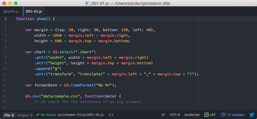
The aforementioned editors have great JavaScript support (or it can be added by using a couple of plugins). The following figure shows how Atom highlights and provides JavaScript support:
Besides editors that support JavaScript, there are also a number of Integrated Development Environments (IDEs) you can use to edit JavaScript. These provide a lot of additional functionality for testing, running, and debugging your code (which we won't touch upon in this book), and also provide a somewhat better JavaScript editing experience. A couple of good IDEs, which have a free or community edition that you can use, are listed as follows:
- WebStorm: This is a great JavaScript IDE (and anything else web related) from IntelliJ. WebStorm is provided in a community edition and a commercial one. For developing JavaScript, the community edition provides all the features that you need. You can get the community edition from here: https://www.jetbrains.com/webstorm/.
- Visual Studio: If you're on a MS Windows system, you might also have a look at the Visual Studio Community edition. It provides JavaScript support out of the box. The Visual Studio Community edition is free to use and can be found here: https://beta.visualstudio.com/vs/community/.
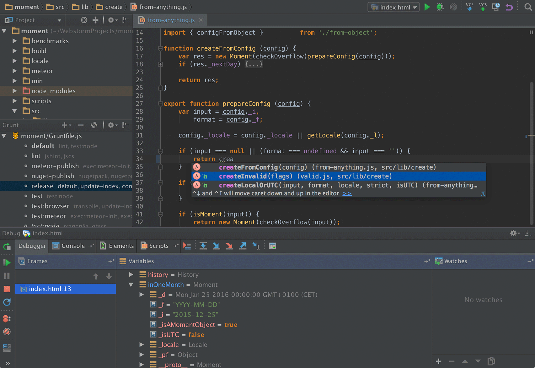
The following screenshot, for example. shows how WebStorm provides code completion for JavaScript:
But, once again, every text editor can be used, since we're just editing standard text files. If you haven't installed an editor yet, now is a good time, since in the next section we'll explain how to get the sources for this book and set up a local web server so you can run the samples.
Getting the sources and setting up a web server
In this section, we'll show you how you can access the sources that are provided together with this book. There are a couple of different ways you can get the sources.
We've got two locations where you can download a zip file with the sources:
- You can download them directly from the Packt Publishing website here: https://www.packtpub.com/books/content/support
- You can alternatively download them from GitHub here: http://github.com/josdirksen/d3dv/archive/master.zip
Once you've downloaded these, just unzip them to a location of your choice. This should result in a directory structure which looks something like this:
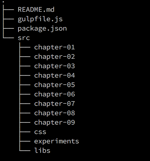
For the rest of this book, we'll reference the directory where you extracted the sources to <DVD3>. We can then use it to point to specific examples or files like this: <DVD3>/src/chapter-01/D01-D01.js.
All the sources of this book can be found on GitHub in the http://github.com/josdirksen/d3dv.git repository. If you've already got Git installed on your machine, you can of course just clone the repository to get access to all the latest sources:
    > git clone https://github.com/josdirksen/d3dv.git
    Cloning into 'd3dv'...
    remote: Counting objects: 3, done.
    remote: Total 3 (delta 0), reused 3 (delta 0), pack-reused 0
    Unpacking objects: 100% (3/3), done.
    Checking connectivity... done.
If you do it this way, you can be sure you'll always have the latest bug fixes and the latest samples. Once you've cloned the repository, the rest of the book can be followed in the same manner. When we mention <DVD3> in this book, in this case it'll point to the cloned repository.
Once you've got the sources extracted to the <DVD3> directory, we could already run some examples by just opening the corresponding HTML file directly. For instance, if you open the <DVD3>/src/chapter-01/D01-01.html file in your browser, you'll see the following results:
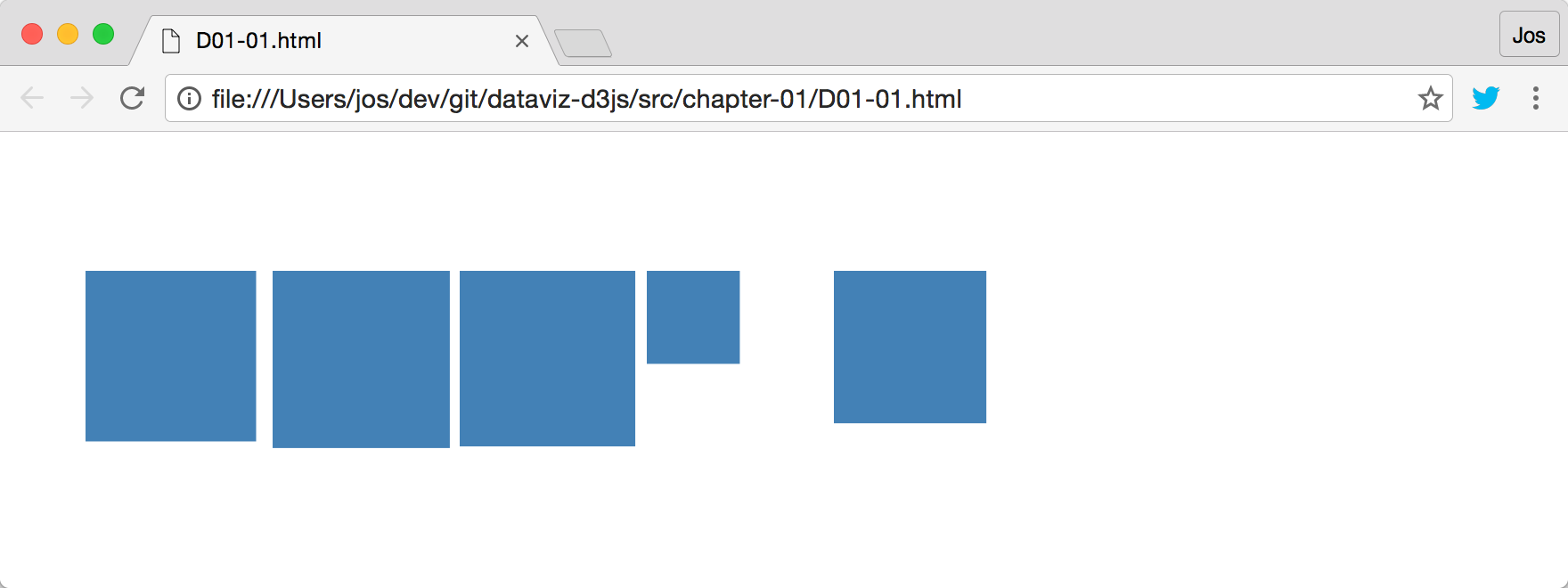
While this will work for the basic examples, this won't work when we're loading external data, due to the restriction that you can't use JavaScript to asynchronously load resources from the local filesystem. To get the examples in this book working, which use external data (most of them), we need to set up a local web server. In the following section, we'll explain how to do this.
Setting up the local web server
There are many options for setting up a local web server. For this book, we've created a simple gulp build file which starts a local web server. The advantage of this web server is that it will automatically reload the browser when any of the sources change, which makes developing D3 visualizations a lot more convenient.
To start this web server, we need to first install node.js, which is required to run our build file. Node.js can be downloaded from here: https://nodejs.org/en/download/. Once you've installed node.js, you need to run the following command once (npm install) in the <DVD3> directory:
    $ npm install
    ├─┬ gulp@3.9.1
    │ ├── archy@1.0.0
    ...
    <removed dependencies for clarity>
    ...
        │ └─┬ websocket-driver@0.6.5
        │   └── websocket-extensions@0.1.1
        ├── livereload-js@2.2.2
        └── qs@5.1.0
You will see a large number of dependencies being downloaded, but once it is done, you can simply start the web server by running the npm start command (also in the <DVD3> directory):
    $ npm start

    > dataviz-d3js@1.0.0 start /Users/jos/dev/git/dataviz-d3js
    > gulp

    [11:20:18] Using gulpfile ~/dev/git/dataviz-d3js/gulpfile.js
    [11:20:18] Starting 'connect'...
    [11:20:18] Finished 'connect' after 30 ms
    [11:20:18] Starting 'watch'...
    [11:20:18] Finished 'watch' after 34 ms
    [11:20:18] Starting 'default'...
    [11:20:18] Finished 'default' after 12 μs
    [11:20:18] Server started http://localhost:8080
    [11:20:18] LiveReload started on port 35729
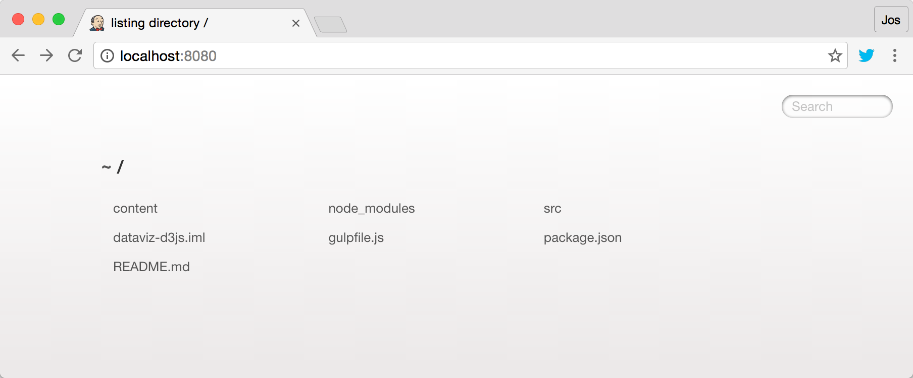
At this point, you've got a web server running at http://localhost:8080. If you now point your browser to this URL, you can access all the examples from your browser:
Basic HTML template
When we create our visualizations, we need to first load the D3 library and the CSS styles that we want to apply. For each of the samples, we'll use the following basic HTML skeleton:
<html>
<head>
    <!-- generic stuff -->
    <script src="../libs/d3.js"></script>
    <script src="../libs/lodash.js"></script>
    <link rel="stylesheet" href="../css/default.css">

    <!-- specific stuff -->
    <script src="./js/D01-01.js"></script>
    <link rel="stylesheet" href="./css/D01-01.css" type="text/css">
</head>
<body>

<div id="output">
    <svg class="chart"></svg>
</div>

<script>
    (function() {
        show();
    })();
</script>

</body>
</html>
This is a standard HTML page, where we first load the complete D3 sources (./libs/d3/js), the lodash JavaScript library, and CSS styles (../css/default.css) that we want to apply to all the examples in this book. We also load the example specific JavaScript (in this example, ./js/D01-01.js) and the example specific CSS (./css/D01-01.css). In this page, we also define a single div tag that has an id with a value output. This is the location in the page where we add our visualizations. A quick note on lodash. Lodash provides a large set of useful collection-related functions, which makes creating and working with JavaScript arrays a lot more convenient. You can see when we use a lodash function when the function call starts with an underscore: for example, _.range(2010, 2016).
There are different ways to load the D3 libraries. In our examples, we load the complete D3 library as a single JavaScript file (the <script src="../libs/d3.js"></script> import). This will load all the APIs provided by D3. D3, however, also comes in a set of micro-libraries, where each library provides a standalone piece of functionality. You can use this to limit the size of the required JavaScript by only including the APIs you need.
Once the page is loaded, the following code block runs, which calls the show function which we'll implement in the example specific JavaScript (./js/D01-01.js in this case):
<script>
    (function() {
        show();
    })();
</script>
The show function implementation will differ for each example, but this way we can keep the basic skeleton the same, and we can focus on JavaScript and the D3 APIs. Note that in this book, we won't explain in detail the JavaScript concepts we use. If you need a reminder on how anonymous functions, closures, variable scope, and so on, work in JavaScript, a great resource is the Mozilla Developer Network (MDN) page on JavaScript: https://developer.mozilla.org/en-US/docs/Web/JavaScript.
How does D3 work?
At this point, you should have a working environment, so let's start by looking at some code and see if we can get D3 up and running. As we've mentioned at the beginning of this chapter, D3 is most often used to create and manipulate SVG elements using a data-driven approach. SVG elements can represent shapes, lines, and also allow for grouping. If you need a reference to check what attributes are available for a specific SVG element, the Mozilla Developer Network also has an excellent page on that: https://developer.mozilla.org/en-US/docs/Web/SVG.
In this section, we'll perform the following steps:
- Create and add an empty SVG group (g) element, to which we'll add our data elements.
- Use a JavaScript array that contains some sample data to add rectangles to the SVG element created in the previous step.
- Show how changes in the data can be used to update the drawn rectangles.
- Explain how to handle added and removed data elements using D3.
At the end of these steps, you should have a decent idea of how D3 binds data to elements, and how you can update the bound data.
Creating a group element
The first thing we need to do is create a g element to which we can add our own elements. Since we're visualizing data using SVG, we need to create this element inside the root SVG element we defined in our HTML skeleton in the previous section. We do this in the following manner:
function show() {

    var margin = { top: 20, bottom: 20, right: 40, left: 40 },
        width = 400 - margin.left - margin.right,
        height = 400 - margin.top - margin.bottom;

    var chart = d3.select(".chart")
        .attr("width", width + margin.left + margin.right)
        .attr("height", height + margin.top + margin.bottom)
        .append("g")
        .attr("transform", "translate(" + margin.left + "," + margin.top + ")");
}
In this code fragment, we see the first usage of the D3 API. We use d3.select to search for the first element with the class chart. This will find the SVG element we defined in our HTML template (<svg class="chart"></svg>), and this will allow us to modify that element. D3 uses a W3C Selectors API string to select elements (more information here: https://www.w3.org/TR/selectors-api/). Summarizing this means that you can use the same kind of selector strings that are also used in CSS to select specific elements:
- .className: selects the elements that have a class with the name className.
- .elemName: selects the elements of type elemName
- #id: selects the element that has an attribute id with a value id.
- .className1 .className2: selects all elements with the class name .className2 which are descendants from the element with class name .className2
Now that we have the SVG element, we use the attr function to set its width and height, leaving a bit of margin at all sides. Finally, we add the g element using the append function and position that element by taking into account the margins we defined by setting the transform attribute. D3 has a fluent API which means we can just chain commands and functions together (as you can see in the previous code fragment). This also means that the result of the final operation is assigned to the chart variable. So in this case, the chart variable is the g element we appended to the svg element.
A g element isn't rendered when you add it to a SVG element. The g element is just a container in which you can add other elements. The most useful part of the g element is that all of the transformations applied to this element are also applied to the children. So if you move the g element, the children will move as well. Additionally, all the attributes defined on this element are inherited by its children.
This might seem like a lot of work to just get an empty group to add elements to, but it is good practice to use a setup like this. Using margins allows us to more easily add axes or legends later on, without having to reposition everything and having a clear and well defined height and weight allows us to use other D3 features (such as scales) to correctly position elements, as we'll see later in this chapter.
At this point, it's also a good point to explain the transform attribute we use to position the g element inside the svg element. The transform attribute allows a couple of operations we can use to change the position and rotation of any SVG elements (such as g, text, rect). You'll see it used throughout this book, since it is the standard way to position SVG elements. The following table shows what can be done with the transform attribute:
| Operation | Description |
| translate(x [y]) | With the translate attribute, we can move the specified element along its X or Y axis. For example, with translate(40 60), we move the specified element 40 pixels to the right and 60 down. If you just want to move an element along the X axis, you can omit the second parameter. |
| scale(x [y]) | The scale operator, as the name implies, allows you to scale an element along the x and y axes. To double the width of an element, you can use scale(1 2), to half the size you use scale(0.5 0.5). Once again, the first parameter is mandatory, and the second one is optional. |
| rotate(a [x] [y]) | The rotate operation allows rotation of the element around a given point (x and y) for a degrees. If the x and y parameters aren't provided, the element is rotated around its center. You can specify a positive a to rotate clockwise (for example, rotate(120)) and a negative value to rotate counter-clockwise (rotate(-10)). |
| skewX(a) / skewY(a) | The skewX and skewY functions allow you to skew (to slant) an element alongside an axis by the specified a degrees: skewX(20) or skewY(-30). |
| matrix(a b c d e f) | The final option you can use is the matrix function. With the matrix operator you can specify an arbitrary matrix operation to be applied to the element. All the previous operations could be written using the matrix operator, but this isn't really that convenient. For instance, we could rewrite translate(40 60) like matrix(1 0 0 1 40 60) |
If you entered this code in your editor and looked at it in your browser you wouldn't really see anything yet. The reason is that we didn't specify a background color (using the fill attribute) for the svg or g element, so the default background color is used. We can, however, check what has happened. We mentioned that besides a good editor to create code, we'll also do a lot of debugging inside the browser, and Chrome has some of the best support. If you open the previous code in your browser, you can already see what is happening when you inspect the elements:

As you can see in this screenshot, the correct attributes have been set on the svg element, a g element is added, and the g element is transformed to position it correctly. If we want to style the svg element, we can use standard CSS for this. For instance, the following code (if added to the css file for this example) will set the background-color attribute of the svg element to black.
svg {
    background-color: black;
}
It is good to understand that CSS styles and element attributes have different priorities. Styles set using the style property have the highest priority, next the styles applied through the CSS classes, and the element properties set directly on the element have the lowest priority.
When we now open the example in the browser, you'll see the svg element as a black rectangle:

At this point, we've got an svg element with a specific size, and one g element to which we'll add other elements in the rest of this example.
Adding rectangles to the group element
In this step, we'll look at the core functionality of D3 which shows how to bind data to elements. We'll create an example that shows a number of rectangles based on some random data. We'll update the data every couple of seconds, and see how we can use D3 to respond to these changes. If you want to look at this example in action, open the example D01-01.html from the chapter 01 folder in your browser. The result looks something like this:

The size and number of rectangles in the screen is randomly determined and the colors indicate whether a rectangle is added or an existing one is updated. If the rectangle is blue, an existing rectangle was selected and updated; if a rectangle is green, it was added to the rectangles already available. It works something like this:
- The first time the rectangles are shown, no rectangles are on screen, so all the rectangles are newly added and colored green. So, for this example, assume we add three rectangles, which, since no rectangles are present, they rendered green.
- After a couple of seconds, the data is updated. Now assume five rectangles need to be rendered. For this, we'll update the three rectangles which are already there with the new data. These are rendered blue since we're updating them. And we add two new rectangles, which are rendered green, just like in the first step.
- After another couple of seconds, the data is updated again. This time we need to render four rectangles. This means updating the first four rectangles, which will turn them blue, and we'll remove the last one, since that one isn't needed anymore.
To accomplish this, we'll first show you the complete code and then step through the different parts:
function show() {
    'use strict';

    var margin = { top: 20, bottom: 20, right: 40, left: 40 },
        width = 800 - margin.left - margin.right,
        height = 400 - margin.top - margin.bottom;

    var chart = d3.select(".chart")
        .attr("width", width + margin.left + margin.right)
        .attr("height", height + margin.top + margin.bottom)
        .append("g")
        .attr("transform", "translate(" + margin.left + ","
                                        + margin.top + ")");

    function update() {

        var rectangleWidth = 100,
        data = [],
            numberOfRectangles = Math.ceil(Math.random() * 7);

        for (var i = 0 ; i < numberOfRectangles ; i++) {
            data.push((Math.random() * rectangleWidth / 2)
                                     + rectangleWidth / 2);
        }

        // Assign the data to the rectangles (should there be any)
        var rectangles = chart.selectAll("rect").data(data);

        // Set a style on the existing rectangles so we can see them
        rectangles.attr("class", "update")
            .attr("width", function(d) {return d})
            .attr("height", function(d) {return d});

        rectangles.enter()
            .append("rect")
            .attr("class", "enter")
            .attr("x", function(d, i) { return i * (rectangleWidth + 5) })
            .attr("y", 50)
            .attr("width", function(d) {return d})
            .attr("height", function(d) {return d});

        // Handle rectangles which are left over
        rectangles.exit().remove();

        // we could also change the ones to be remove
        // rectangles
        //     .exit()
        //     .attr("class", "remove");
    }

    // set initial value
    update();
    // and update every 3 seconds
    d3.interval(function() { update(); }, 3000);
}
In the beginning of this function, you once again see the code we use to create and set up our SVG and main g elements. Let's ignore that and move on to the update() function. When this function is called it will take a couple of steps:
Creating dummy data
The first thing it does is that it creates some dummy data. This is the data that determines how many rectangles to render, and how large the rectangles will be:
var rectangleWidth = 100,
    data = [],
    numberOfRectangles = Math.ceil(Math.random() * 7);

for (var i = 0 ; i < numberOfRectangles ; i++) {
    data.push((Math.random() * rectangleWidth / 2)
                             + rectangleWidth / 2);
}
This is just plain JavaScript, and this will result in the data array being filled with one to seven numeric values ranging from 50 to 100. It could look something like this:
[52.653238934888726, 88.52709144102309, 81.70794256804369, 58.10611357491862]
Binding the data and updating existing rectangles
The next step is assigning this data to a D3 selection. We do this by using the selectAll function on the chart variable we defined earlier (remember this is the main g element, we added initially):
var rectangles = chart.selectAll("rect").data(data);
This call will select all the rectangles which are already appended as children to the chart variable. The first time this is called, rectangles will have no children, but on subsequent calls this will select any rectangles that have been added in the previous call to the update() function. To differentiate between newly added rectangles and rectangles which we'll reuse, we add a specific CSS class. Besides just adding the CSS class, we also need to make sure they have the correct width and height properties set, since the bound data has changed.
In the case of rectangles which we reuse, we do that like this:
rectangles.attr("class", "update")
          .attr("width", function(d) {return d})
          .attr("height", function(d) {return d});
To set the CSS we use the attr function to set the class property, which points to a style defined in our CSS file. The width and height properties are set in the same manner, but their value is based on the value of the passed data. You can do this by setting the value of that attribute to a function(d) {...}. The d which is passed in to this function is the value of the corresponding element from the bound data array. So the first rectangle which is found is bound to data[0], the second to data[1], and so on. In this case, we set both the width and the height of the rectangle to the same value.
The CSS for this class is very simple, and just makes sure that the newly added rectangles are filled with a nice blue color:
.update {
    fill: steelblue;
}
Adding new rectangles if needed
At this point, we've only updated the style and dimensions of the rectangles which are updated. We repeat pretty much the same process for the rectangles that need to be created. This happens when our data array is larger than the number of rectangles we can find:
rectangles.enter()
    .append("rect")
    .attr("class", "enter")
    .attr("x", function(d, i) { return i * (rectangleWidth + 5) })
    .attr("y", 50)
    .attr("width", function(d) {return d})
    .attr("height", function(d) {return d});
Not that different from the update call, but this time we first call the enter() function and then create the SVG element we want to add like this: .append("rect"). After the append call, we configure the rectangle and set its class, width, and height properties, just like we did in the previous section (this time the CSS will render the newly added rectangle in green). If you look at the code, you can see that we also set the position of this element by setting the x and y attributes of the added rectangle. This is needed since this is the first time this rectangle is added, and we need to determine where to position it. We fix the y position to 50, but need to make the x position dependent on the position of the element from the data array to which it is bound. We once again bind the attribute to a function. This time we specify a function with two arguments: function(d, i) {...}. The first one is the element from the data array, and the second argument (i), is the position in the data array. So the first element has i = 0, the second i = 1, and so on. Now, when we add a new rectangle we calculate its x position by just multiplying its array position with the maximum rectangleWidth and add a couple of pixels margin. This way none of our rectangles will overlap.
If you look at the code for adding new elements, and updating existing ones, you might notice some duplicate code. In both instances, we use .attr to set the width and the height properties. If we'd wanted to, we could remove this duplication by using the .merge function. The code to set the new width and height for the new elements and the updated ones would then look like this:
rectangles.attr("class", "update");

rectangles.enter()
    .append("rect")
    .attr("class", "enter")
    .attr("x", function(d, i) { return i * (rectangleWidth + 5) })
    .attr("y", 50)
    .merge(rectangles)
    .attr("width", function(d) {return d})
    .attr("height", function(d) {return d});
This means that after merging the new and updated elements together, on that combined set, we use the .attr function to set the width and the height property. Personally, I'd like to keep these steps separate, since it is more clear what happens in each of the steps.
Removing elements which aren't needed anymore
The final step we need to take is to remove rectangles that aren't needed anymore. If in the first call to update we add five rectangles, and in the next call only three are needed, we're stuck with two leftover ones. D3 also has an elegant mechanism to deal with that:
rectangles.exit().remove();
The call to exit() will select the elements for which no data is available. We can then do anything we want with those rectangles. In this case, we just remove them by calling remove(), but we could also change their opacity to make them look transparent, or animate them to slowly disappear.
For instance, if we replace the previous line of code with this:
rectangles.exit().attr("class", "remove");
Then set the CSS for the remove class to this:
.remove {
    fill: red;
    opacity: 0.2;
}
In that case, we'd see the following:

In the preceding screenshot, we've reused two existing rectangles, and instead of removing the five we don't need, we change their style to the remove class, which renders them semi-transparent red.
Visualizing our first data
So far we've seen the basics of how D3 works. In this last section of this first chapter, we'll create a simple visualization of some real data. We're going to visualize the popularity of baby names in the USA. The final result will look this:

As you can see in this figure, we create pink bars for the girl names, blue bars for the boy names, and add an axis at the top and the bottom, which shows the number of times that name was chosen. The first thing, though, is take a look at the data.
Sanitizing and getting the data
For this example, we'll download data from https://www.ssa.gov/oact/babynames/limits.html. This site provides data for all the baby names in the US since 1880. On this page, you can find national data and state-specific data. For this example, download the national data dataset. Once you've downloaded it, you can extract it, and you'll see data for a lot of different years:
$ ls -1
NationalReadMe.pdf
yob1880.txt
yob1881.txt
yob1882.txt
yob1883.txt
yob1884.txt
yob1885.txt
...
yob2013.txt
yob2014.txt
yob2015.txt
As you can see, we have data from 1880 until 2015. For this example, I've used the data from 2015, but you can use pretty much anything you want. Now let's look a bit closer at the data:
$ cat yob2015.txt
Emma,F,20355
Olivia,F,19553
Sophia,F,17327
Ava,F,16286
Isabella,F,15504
Mia,F,14820
Abigail,F,12311
Emily,F,11727
Charlotte,F,11332
Harper,F,10241
...
Zynique,F,5
Zyrielle,F,5
Noah,M,19511
Liam,M,18281
Mason,M,16535
Jacob,M,15816
William,M,15809
Ethan,M,14991
James,M,14705
Alexander,M,14460
Michael,M,14321
Benjamin,M,13608
Elijah,M,13511
Daniel,M,13408
In this data, we've got a large number of rows where each row shows the name and the sex (M or F). First, all the girls' names are shown, and after that all the boys' names are shown. The data in itself already looks pretty usable, so we don't need to do much processing before we can use it. The only thing, though, we do is add a header to this file, so that it looks like this:
name,sex,amount
Emma,F,20355
Olivia,F,19553
Sophia,F,17327
Ava,F,16286
This will make parsing this data into D3 a little bit easier, since the default way of parsing CSV data with D3 assumes the first line is a header. The sanitized data we use in this example can be found here: <DVD3>/src/chapter-01/data/yob2015.txt.
Creating the visualization
Now that we've got the data we want to work with, we can start creating the example. The files used in this example are the following:
- <DVD3>/src/chapter-01/D01-02.html: The HTML template that loads the correct CSS and JavaScript files for this example
- <DVD3>/src/chapter-01/js/D01-02.js: The JavaScript which uses the D3 APIs to draw the chart
- <DVD3>/src/chapter-01/css/D01-02.css: Custom CSS to color the bars and format the text elements
- <DVD3>/src/chapter-01/data/yob2015.txt: The data that is visualized
Let's start with the complete JavaScript file first. It might seem complex, and it introduces a couple of new concepts, but the general idea should be clear from the code (if you open the source file in your editor, you can also see inline comments for additional explanation):
function show() {
    'use strict';

    var margin = { top: 30, bottom: 20, right: 40, left: 40 },
        width = 800 - margin.left - margin.right,
        height = 600 - margin.top - margin.bottom;

    var chart = d3.select('.chart')
        .attr('width', width + margin.left + margin.right)
        .attr('height', height + margin.top + margin.bottom)
        .append('g')
        .attr('transform', 'translate(' + margin.left + ','
                                        + margin.top + ')');

    var namesToShow = 10;
    var barWidth = 20;
    var barMargin = 5;

    d3.csv('data/yob2015.txt', function (d) { return { name: d.name, sex: d.sex, amount: +d.amount }; }, function (data) {
        var grouped = _.groupBy(data, 'sex');
        var top10F = grouped['F'].slice(0, namesToShow);
        var top10M = grouped['M'].slice(0, namesToShow);

        var both = top10F.concat(top10M.reverse());

        var bars = chart.selectAll("g").data(both)
            .enter()
            .append('g')
            .attr('transform', function (d, i) {
                var yPos = ((barWidth + barMargin) * i);
                return 'translate( 0 ' + yPos +  ')';
            });

        var yScale = d3.scaleLinear()
            .domain([0, d3.max(both, function (d) { return d.amount; })])
            .range([0, width]);

        bars.append('rect')
            .attr("height", barWidth)
            .attr("width", function (d) { return yScale(d.amount); })
            .attr("class", function (d) { return d.sex === 'F' ? 'female' : 'male'; });

        bars.append("text")
            .attr("x", function (d) { return yScale(d.amount) - 5 ; })
            .attr("y", barWidth / 2)
            .attr("dy", ".35em")
            .text(function(d) { return d.name; });

        var bottomAxis = d3.axisBottom().scale(yScale).ticks(20, "s");
        var topAxis = d3.axisTop().scale(yScale).ticks(20, "s");

        chart.append("g")
            .attr('transform', 'translate( 0 ' + both.length * (barWidth + barMargin) +  ')')
            .call(bottomAxis);

        chart.append("g")
            .attr('transform', 'translate( 0 ' + -barMargin + ' )')
            .call(topAxis);
    });
}
In this JavaScript file, we perform the following steps:
- Set up the main chart element, like we did in the previous example.
- Load the data from the CSV file using d3.csv.
- Group the loaded data so we only have the top 10 names for both sexes. Note that we use the groupBy function from the lodash library (https://lodash.com/) for this. This library provides a lot of additional functions to deal with common array operations. Throughout this book, we'll use this library in places where the standard JavaScript APIs don't provide enough functionality.
- Add g elements that will hold the rect and text elements for each name.
- Create the rect elements with the correct width corresponding to the number of times the name was used.
- Create the text elements to show the name at the end of the rect elements.
- Add some CSS styles for the rect and text elements.
- Add an axis to the top and the bottom for easy referencing.
We'll skip the first step since we've already explained that before, and move on to the usage of the d3.csv API call. Before we do that, there are a couple of variables in the JavaScript that determine how the bars look, and how many we show:
var namesToShow = 10;
var barWidth = 20;
var barMargin = 5;
These variables will be used throughout the explanation in the following sections. What this means is that we're going to show 10 (namesToShow) names, a bar is 20 (barWidth) pixels wide, and between each bar we put a five pixel margin.
Loading CSV data with D3
To load data asynchronously, D3 provides a number of helper functions. In this case, we've used the d3.csv function:
d3.csv('data/yob2015.txt',
        function (d) { return { name: d.name, sex: d.sex, amount: +d.amount }; },
        function (data) {
        ...
        }
The d3.csv function we use takes three parameters. The first one, data/yob2015.txt, is a URL which points to the data we want to load. The second argument is a function that is applied to each row read by D3. The object that's passed into this function is based on the header row of the CSV file. In our case, this data looks like this:
{
    name: 'Sophie',
    sex: 'F',
    amount: '1234'
}
This (optional) function allows you to modify the data in the row, before it is passed on as an array (data) to the last argument of the d3.csv function. In this example, we use this second argument to convert the string value d.amount to a numeric value. Once the data is loaded and in this case converted, the function provided as the third argument is called with an array of all the read and converted values, ready for us to visualize the data.
D3 provides a number of functions like d3.csv to load data and resources. These are listed in the following table:
| Function | Description |
| d3.csv(url, [row], callback) | Retrieve a CSV file, optionally pass each row through the row function. When done the callback function is called with all the read data. |
| d3.tsv(url, [row], callback) | Retrieve a TSV (same as a CSV file but separated by tabs) file, optionally pass each row through the row function. When done the callback function is called with all the read data. |
| d3.html(url, callback) | Get a HTML file, and pass it into the callback function when loaded. |
| d3.json(url, callback) | Get a JSON file, and pass it into the callback function when loaded. |
| d3.text(url, callback) | Get a basic test file, and pass it into the callback function when loaded. |
| d3.xml(url, [row], callback) | Get an XML file, and pass it into the callback function when loaded. |
You can also manually process CSV files if they happen to use a different format. You should load those using the d3.text function, and use any of the functions from the d3-dsv module to parse the data. You can find more information on the d3-dsv module here: https://github.com/d3/d3-dsv.
Grouping the loaded data so we only have the top 10 names for both sexes
At this point, we've only loaded the data. If you look back at the figure, you can see that we create a chart using the top 10 female and male names. With the following lines of code, we convert the big incoming data array to an array that contains just the top 10 female and male names:
var grouped = _.groupBy(data, 'sex');
var top10F = grouped['F'].slice(0, namesToShow);
var top10M = grouped['M'].slice(0, namesToShow);

var both = top10F.concat(top10M.reverse());
Here we use the lodash's groupBy function,to sort our data based on the sex property of each row. Next we take the first 10 (namesToShow) elements from the grouped data, and create a single array from them using the concat function. We also reverse the top10M array to make the highest boy's name appear at the bottom of the chart (as you can see when you look at the example).
Adding group elements
At this point, we've got the data into a form that we can use. The next step is to create a number of containers, to which we can add the rect that represents the number of times the name was used, and we'll also add a text element there that displays the name:
var bars = chart.selectAll("g").data(both)
    .enter()
    .append('g')
    .attr('transform', function (d, i) {
        var yPos = ((barWidth + barMargin) * i);
        return 'translate( 0 ' + yPos +  ')';
    });
Here, we bind the both array to a number of g elements. We only need to use the enter function here, since we know that there aren't any g elements that can be reused. We position each g element using the translate operation of the transform attribute. We translate the g element along its y-axis based on the barWidth, the barMargin, and the position of the data element (d) in our data (both) array. If you use the Chrome developer tools, you'll see something like this, which nicely shows the calculated translate values:

All that is left to do now, is draw the rectangles and add the names.
Adding the bar chart and baby name
In the previous section, we added the g elements and assigned those to the bars variable. In this section, we're going to calculate the width of the individual rectangles and add those and some text to the g:
var yScale = d3.scaleLinear()
    .domain([0, d3.max(both, function (d) { return d.amount; })])
    .range([0, width]);

bars.append('rect')
    .attr("height", barWidth)
    .attr("width", function (d) { return yScale(d.amount); })
    .attr("class", function (d) { return d.sex === 'F' ? 'female' : 'male'; });

bars.append("text")
    .attr("x", function (d) { return yScale(d.amount) - 5 ; })
    .attr("y", barWidth / 2)
    .attr("dy", ".35em")
    .text(function(d) { return d.name; });
Here we see something new: the d3.scaleLinear function. With a d3.scaleLinear, we can let D3 calculate how the number of times a name was given (the amount property) maps to a specific width. We want to use the full width (width property, which has a value of 720) of the chart for our bars, so that would mean that the highest value in our input data should map to that value:
- The name Emma, which occurred 20355 times, should map to a value of 720
- The name Olivia, which occurred 19553 times, should map to a value of 720 * (19553/20355)
- The name Mia, which occurred 14820 times, should map to a value of 720 * (14820/20355)
- And so on...
Now, we could calculate this ourselves and set the size of the rect accordingly, but using the d3.scaleLinear is much easier, and provides additional functionality. Let's look at the definition a bit closer:
var yScale = d3.scaleLinear()
    .domain([0, d3.max(both, function (d) { return d.amount; })])
    .range([0, width]);
What we do here, is we define a linear scale, whose input domain is set from 0 to the maximum amount in our data. This input domain is mapped to an output range starting at 0 and ending at width. The result, yScale, is a function which we can now use to map the input domain to the output range: for example, yScale(1234) returns 43.64922623434046.
Once you've got a scale, you can use a couple of functions to change its behavior:
| Function | Description |
| invert(val) | This function expects a value of the output domain, and returns the corresponding value from the input domain. |
| rangeRound() | You can use this instead of the range option we saw earlier. With this function, the scale only returns rounded values. |
| clamp(bool) | With the clamp function, you define the behavior of what happens when a value is passed in which is outside the input domain. In the case where clamp is true, the minimal or maximum output value is returned. In the case where clamp is false, an output value is calculated normally, which will result in a value outside the output domain. |
| ticks([count]) | This function returns a number of ticks (10 is the default), which can be used to create an axis, or reference lines. |
| nice([ticks]) | This function rounds the first and last value of the input domain. You can optionally specify a number of ticks you want to return, and the rounding function will take those into account. |
This is just a small part of the scales support provided by D3. In the rest of the book, we'll explore more of the scales options that are available.
With the scale defined, we can use that to create our rect and text elements in the same way we did in our previous example:
bars.append('rect')
    .attr("height", barWidth)
    .attr("width", function (d) { return yScale(d.amount); })
    .attr("class", function (d) { return d.sex === 'F' ? 'female' : 'male'; });
Here we create a rect with a fixed height, and a width which is defined by the yScale and the number of times the name was used. We also add a class to the rect so that we can set its colors (and other styling attributes) through CSS. In the case where sex is F, we set the class female and in the other case we set the class male.
To position the text element, we do pretty much the same:
bars.append("text")
    .attr("class", "label")
    .attr("x", function (d) { return yScale(d.amount) - 5 ; })
    .attr("y", barWidth / 2)
    .attr("dy", ".35em")
    .text(function(d) { return d.name; });
We create a new text element, position it at the end of the bar, set a custom CSS class, and finally set its value to d.name. The dy attribute might seem a bit strange, but this allows us to position the text nicely in the middle of the bar chart. If we opened the example at this point, we'd see something like this:

We can see that all the information is in there, but it still looks kind of ugly. In the following section, we add some CSS to improve what the chart looks like.
Adding some CSS classes to style the bars and text elements
When we added the rect elements, we added a female class attribute for the girls' names, and a male one for the boys' names and we've also set the style of our text elements to label. In our CSS file, we can now define colors and other styles based on these classes:
.male {
    fill: steelblue;
}

.female {
    fill: hotpink;
}

.label {
    fill: black;
    font: 10px sans-serif;
    text-anchor: end;
}
With these CSS properties, we set the fill color of our rectangles. The elements with the male class will be filled steelblue and the elements with the female class will be filled hotpink. We also change how the elements with the .label class are rendered. For these elements, we change the font and the text-anchor. The text-anchor, especially, is important here, since it makes sure that the text element's right side is positioned at the x and y value, instead of the left side. The effect is that the text element is nicely aligned at the end of our bars.
Adding the axis on the top and bottom
The final step we need to take to get the figure from the beginning of this section is to add the top and bottom axes. D3 provides you with a d3.axis<orientation> function, which allows you to create an axis at the bottom, top, left, or right side. When creating an axis, we pass in a scale (which we also used for the width of the rectangles), and tell D3 how the axis should be formatted. In this case, we want 20 ticks, and use the s formatting, which tells D3 to use the international system of units (SI).
This means that D3 will use metric prefixes to format the tick values (more info can be found here: https://en.wikipedia.org/wiki/Metric_prefix).
var bottomAxis = d3.axisBottom().scale(yScale).ticks(20, "s");
var topAxis = d3.axisTop().scale(yScale).ticks(20, "s");

chart.append("g")
    .attr('transform', 'translate( 0 ' + both.length * (barWidth + barMargin) +  ')')
    .call(bottomAxis);

chart.append("g")
    .attr('transform', 'translate( 0 ' + -barMargin + ' )')
    .call(topAxis);
And with that, we've recreated the example we saw at the beginning of this section:

If you look back at the code we showed at the beginning of this section, you can see that we only need a small number of lines of code to create a nice visualization.
Summary
In this chapter, we've set up our working environment and introduced the first couple of concepts of D3. We've showed that there is a standard pattern for binding data to elements, and how we can use D3 to handle new elements, update existing elements, and how to remove obsolete elements. We've also created our first visualization in this chapter. We've used a standard CSV file, and converted that to a bar chart, complete with custom colors, text elements, and a set of axes. Throughout this chapter, we've touched upon a couple of D3 APIs and concepts, such as d3.selectAll, d3.axisBottom, and even explored a part of how D3 handles scales (d3.linearScale).
In the next chapter, we'll continue with the subjects we've seen so far, and look more closely at how you can use D3 to create different kinds of charts.


