Download code from GitHub
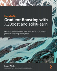
Chapter 1: Machine Learning Landscape
Welcome to Hands-On Gradient Boosting with XGBoost and Scikit-Learn, a book that will teach you the foundations, tips, and tricks of XGBoost, the best machine learning algorithm for making predictions from tabular data.
The focus of this book is XGBoost, also known as Extreme Gradient Boosting. The structure, function, and raw power of XGBoost will be fleshed out in increasing detail in each chapter. The chapters unfold to tell an incredible story: the story of XGBoost. By the end of this book, you will be an expert in leveraging XGBoost to make predictions from real data.
In the first chapter, XGBoost is presented in a sneak preview. It makes a guest appearance in the larger context of machine learning regression and classification to set the stage for what's to come.
This chapter focuses on preparing data for machine learning, a process also known as data wrangling. In addition to building machine learning models, you will learn about using efficient Python code to load data, describe data, handle null values, transform data into numerical columns, split data into training and test sets, build machine learning models, and implement cross-validation, as well as comparing linear regression and logistic regression models with XGBoost.
The concepts and libraries presented in this chapter are used throughout the book.
This chapter consists of the following topics:
Previewing XGBoost
Wrangling data
Predicting regression
Predicting classification
Previewing XGBoost
Machine learning gained recognition with the first neural network in the 1940s, followed by the first machine learning checker champion in the 1950s. After some quiet decades, the field of machine learning took off when Deep Blue famously beat world chess champion Gary Kasparov in the 1990s. With a surge in computational power, the 1990s and early 2000s produced a plethora of academic papers revealing new machine learning algorithms such as random forests and AdaBoost.
The general idea behind boosting is to transform weak learners into strong learners by iteratively improving upon errors. The key idea behind gradient boosting is to use gradient descent to minimize the errors of the residuals. This evolutionary strand, from standard machine learning algorithms to gradient boosting, is the focus of the first four chapters of this book.
XGBoost is short for Extreme Gradient Boosting. The Extreme part refers to pushing the limits of computation to achieve gains in accuracy and speed. XGBoost's surging popularity is largely due to its unparalleled success in Kaggle competitions. In Kaggle competitions, competitors build machine learning models in attempts to make the best predictions and win lucrative cash prizes. In comparison to other models, XGBoost has been crushing the competition.
Understanding the details of XGBoost requires understanding the landscape of machine learning within the context of gradient boosting. In order to paint a full picture, we start at the beginning, with the basics of machine learning.
What is machine learning?
Machine learning is the ability of computers to learn from data. In 2020, machine learning predicts human behavior, recommends products, identifies faces, outperforms poker professionals, discovers exoplanets, identifies diseases, operates self-driving cars, personalizes the internet, and communicates directly with humans. Machine learning is leading the artificial intelligence revolution and affecting the bottom line of nearly every major corporation.
In practice, machine learning means implementing computer algorithms whose weights are adjusted when new data comes in. Machine learning algorithms learn from datasets to make predictions about species classification, the stock market, company profits, human decisions, subatomic particles, optimal traffic routes, and more.
Machine learning is the best tool at our disposal for transforming big data into accurate, actionable predictions. Machine learning, however, does not occur in a vacuum. Machine learning requires rows and columns of data.
Data wrangling
Data wrangling is a comprehensive term that encompasses the various stages of data preprocessing before machine learning can begin. Data loading, data cleaning, data analysis, and data manipulation are all included within the sphere of data wrangling.
This first chapter presents data wrangling in detail. The examples are meant to cover standard data wrangling challenges that can be swiftly handled by pandas, Python's special library for handling data analytics. Although no experience with pandas is required, basic knowledge of pandas will be beneficial. All code is explained so that readers new to pandas may follow along.
Dataset 1 – Bike rentals
The bike rentals dataset is our first dataset. The data source is the UCI Machine Learning Repository (https://archive.ics.uci.edu/ml/index.php), a world-famous data warehouse that is free to the public. Our bike rentals dataset has been adjusted from the original dataset (https://archive.ics.uci.edu/ml/datasets/bike+sharing+dataset) by sprinkling in null values so that you can gain practice in correcting them.
Accessing the data
The first step in data wrangling is to access the data. This may be achieved with the following steps:
Download the data. All files for this book have been stored on GitHub. You may download all files to your local computer by pressing the Clone button. Here is a visual:

Figure 1.1 – Accessing data
After downloading the data, move it to a convenient location, such as a
Datafolder on your desktop.Open a Jupyter Notebook. You will find the link to download Jupyter Notebooks in the preface. Click on Anaconda, and then click on Jupyter Notebooks. Alternatively, type
jupyter notebookin the terminal. After the web browser opens, you should see a list of folders and files. Go to the same folder as the bike rentals dataset and select New: Notebook: Python 3. Here is a visual guide:
Figure 1.2 – Visual guide to accessing the Jupyter Notebook
Tip
If you are having difficulties opening a Jupyter Notebook, see Jupyter's official trouble-shooting guide: https://jupyter-notebook.readthedocs.io/en/stable/troubleshooting.html.
Enter the following code in the first cell of your Jupyter Notebook:
import pandas as pd
Press Shift + Enter to run the cell. Now you may access the
pandaslibrary when you writepd.Load the data using
pd.read_csv. Loading data requires areadmethod. Thereadmethod stores the data as a DataFrame, apandasobject for viewing, analyzing, and manipulating data. When loading the data, place the filename in quotation marks, and then run the cell:df_bikes = pd.read_csv('bike_rentals.csv')If your data file is in a different location than your Jupyter Notebook, you must provide a file directory, such as
Downloads/bike_rental.csv.Now the data has been properly stored in a DataFrame called
df_bikes.Tip
Tab completion: When coding in Jupyter Notebooks, after typing a few characters, press the Tab button. For CSV files, you should see the filename appear. Highlight the name with your cursor and press Enter. If the filename is the only available option, you may press Enter. Tab completion will make your coding experience faster and more reliable.
Display the data using
.head(). The final step is to view the data to ensure that it has loaded correctly..head()is a DataFrame method that displays the first five rows of the DataFrame. You may place any positive integer in parentheses to view any number of rows. Enter the following code and press Shift + Enter:df_bikes.head()
Here is a screenshot of the first few lines along with the expected output:
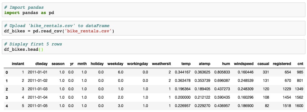
Figure 1.3 –The bike_rental.csv output
Now that we have access to the data, let's take a look at three methods to understand the data.
Understanding the data
Now that the data has been loaded, it's time to make sense of the data. Understanding the data is essential to making informed decisions down the road. Here are three great methods for making sense of the data.
.head()
You have already seen .head(), a widely used method to interpret column names and numbers. As the preceding output reveals, dteday is a date, while instant is an ordered index.
.describe()
Numerical statistics may be viewed by using .describe() as follows:
df_bikes.describe()
Here is the expected output:
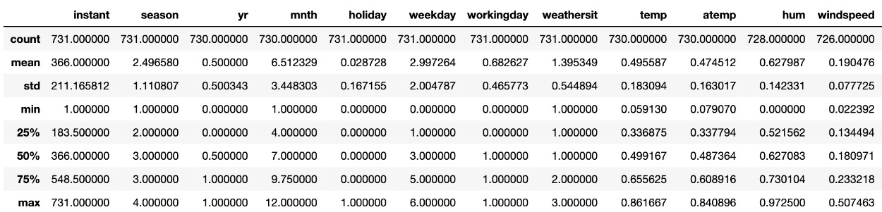
Figure 1.4 – The .describe() output
You may need to scroll to the right to see all of the columns.
Comparing the mean and median (50%) gives an indication of skewness. As you can see, mean and median are close to one another, so the data is roughly symmetrical. The max and min values of each column, along with the quartiles and standard deviation (std), are also presented.
.info()
Another great method is .info(), which displays general information about the columns and rows:
df_bikes.info()
Here is the expected output:
<class 'pandas.core.frame.DataFrame'>
RangeIndex: 731 entries, 0 to 730
Data columns (total 16 columns):
 #   Column      Non-Null Count  Dtype
---  ------      --------------  -----
 0   instant     731 non-null    int64
 1   dteday      731 non-null    object
 2   season      731 non-null    float64
 3   yr          730 non-null    float64
 4   mnth        730 non-null    float64
 5   holiday     731 non-null    float64
 6   weekday     731 non-null    float64
 7   workingday  731 non-null    float64
 8   weathersit  731 non-null    int64
 9   temp        730 non-null    float64
 10  atemp       730 non-null    float64
 11  hum         728 non-null    float64
 12  windspeed   726 non-null    float64
 13  casual      731 non-null    int64
 14  registered  731 non-null    int64
 15  cnt         731 non-null    int64
dtypes: float64(10), int64(5), object(1)
memory usage: 91.5+ KB
As you can see, .info() gives the number of rows, number of columns, column types, and non-null values. Since the number of non-null values differs between columns, null values must be present.
Correcting null values
If null values are not corrected, unexpected errors may arise down the road. In this subsection, we present a variety of methods that may be used to correct null values. Our examples are designed not only to handle null values but also to highlight the breadth and depth of pandas.
The following methods may be used to correct null values.
Finding the number of null values
The following code displays the total number of null values:
df_bikes.isna().sum().sum()
Here is the outcome:
12
Note that two .sum() methods are required. The first method sums the null values of each column, while the second method sums the column counts.
Displaying null values
You can display all rows containing null values with the following code:
df_bikes[df_bikes.isna().any(axis=1)]
This code may be broken down as follows: df_bikes[conditional] is a subset of df_bikes that meets the condition in brackets. .df_bikes.isna().any gathers any and all null values while (axis=1) specifies values in the columns. In pandas, rows are axis 0 and columns are axis 1.
Here is the expected output:
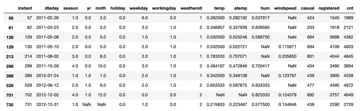
Figure 1.5 – Bike Rentals dataset null values
As you can see from the output, there are null values in the windspeed, humidity, and temperature columns along with the last row.
Tip
If this is your first time working with pandas, it may take time to get used to the notation. Check out Packt's Hands-On Data Analysis with Pandas for a great introduction: https://subscription.packtpub.com/book/data/9781789615326.
Correcting null values
Correcting null values depends on the column and dataset. Let's go over some strategies.
Replacing with the median/mean
One common strategy is to replace null values with the median or mean. The idea here is to replace null values with the average column value.
For the 'windspeed' column, the null values may be replaced with the median value as follows:
df_bikes['windspeed'].fillna((df_bikes['windspeed'].median()), inplace=True)
df_bikes['windspeed'].fillna means that the null values of the 'windspeed' column will be filled. df_bikes['windspeed'].median() is the median of the 'windspeed' column. Finally, inplace=True ensures that the changes are permanent.
Tip
The median is often a better choice than the mean. The median guarantees that half the data is greater than the given value and half the data is lower. The mean, by contrast, is vulnerable to outliers.
In the previous cell, df_bikes[df_bikes.isna().any(axis=1)] revealed rows 56 and 81 with null values for windspeed. These rows may be displayed using .iloc, short for index location:
df_bikes.iloc[[56, 81]]
Here is the expected output:

Figure 1.6 – Rows 56 and 81
As expected, the null values have been replaced with the windspeed median.
Tip
It's common for users to make mistakes with single or double brackets when using pandas. .iloc uses single brackets for one index as follows: df_bikes.iloc[56]. Now, df_bikes also accepts a list inside brackets to allow multiple indices. Multiple indices require double brackets as follows: df_bikes.iloc[[56, 81]]. Please see https://pandas.pydata.org/pandas-docs/stable/reference/api/pandas.DataFrame.iloc.html for further documentation.
Groupby with the median/mean
It's possible to get more nuanced when correcting null values by using a groupby.
A groupby organizes rows by shared values. Since there are four shared seasons spread out among the rows, a groupby of seasons results in a total of four rows, one for each season. But each season comes from many different rows with different values. We need a way to combine, or aggregate, the values. Choices for the aggregate include .sum(), .count(), .mean(), and .median(). We use .median().
Grouping df_bikes by season with the .median() aggregate is achieved as follows:
df_bikes.groupby(['season']).median()
Here is the expected output:
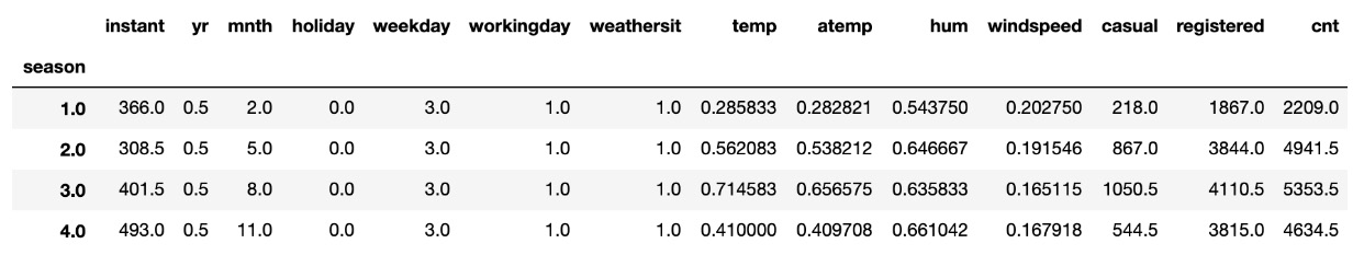
Figure 1.7 – The output of grouping df_bikes by season
As you can see, the column values are the medians.
To correct the null values in the hum column, short for humidity, we can take the median humidity by season.
The code for correcting null values in the hum column is df_bikes['hum'] = df_bikes['hum'].fillna().
The code that goes inside fillna is the desired values. The values obtained from groupby require the transform method as follows:
df_bikes.groupby('season')['hum'].transform('median')
Here is the combined code in one long step:
df_bikes['hum'] = df_bikes['hum'].fillna(df_bikes.groupby('season')['hum'].transform('median'))
You may verify the transformation by checking df_bikes.iloc[[129, 213, 388]].
Obtaining the median/mean from specific rows
In some cases, it may be advantageous to replace null values with data from specific rows.
When correcting temperature, aside from consulting historical records, taking the mean temperature of the day before and the day after should give a good estimate.
To find null values of the 'temp' column, enter the following code:
df_bikes[df_bikes['temp'].isna()]
Here is the expected output:

Figure 1.8 – The output of the 'temp' column
As you can see, index 701 contains null values.
To find the mean temperature of the day before and the day after the 701 index, complete the following steps:
Sum the temperatures in rows
700and702and divide by2. Do this for the'temp'and'atemp'columns:mean_temp = (df_bikes.iloc[700]['temp'] + df_bikes.iloc[702]['temp'])/2 mean_atemp = (df_bikes.iloc[700]['atemp'] + df_bikes.iloc[702]['atemp'])/2
Replace the null values:
df_bikes['temp'].fillna((mean_temp), inplace=True)
df_bikes['atemp'].fillna((mean_atemp), inplace=True)
You may verify on your own that the null values have been filled as expected.
Extrapolate dates
Our final strategy to correct null values involves dates. When real dates are provided, date values may be extrapolated.
df_bikes['dteday'] is a date column; however, the type of column revealed by df_bikes.info() is an object, commonly represented as a string. Date objects such as years and months must be extrapolated from datetime types. df_bikes['dteday'] may be converted to a 'datetime' type using the to_datetime method, as follows:
df_bikes['dteday'] = pd.to_datetime(df_bikes['dteday'],infer_datetime_format=True)
infer_datetime_format=True allows pandas to decide the kind of datetime object to store, a safe option in most cases.
To extrapolate individual columns, first import the datetime library:
import datetime as dt
We can now extrapolate dates for the null values using some different approaches. A standard approach is convert the 'mnth' column to the correct months extrapolated from the 'dteday' column. This has the advantage of correcting any additional errors that may have surfaced in conversions, assuming of course that the 'dteday' column is correct.
The code is as follows:
ddf_bikes['mnth'] = df_bikes['dteday'].dt.month
It's important to verify the changes. Since the null date values were in the last row, we can use .tail(), a DataFrame method similar to .head(), that shows the last five rows:
df_bikes.tail()
Here is the expected output:
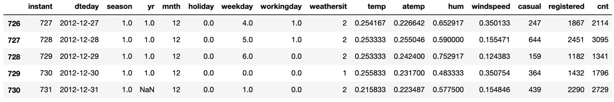
Figure 1.9 – The output of the extrapolated date values
As you can see, the month values are all correct, but the year value needs to be changed.
The years of the last five rows in the 'dteday' column are all 2012, but the corresponding year provided by the 'yr' column is 1.0. Why?
The data is normalized, meaning it's converted to values between 0 and 1.
Normalized data is often more efficient because machine learning weights do not have to adjust for different ranges.
You can use the .loc method to fill in the correct value. The .loc method is used to locate entries by row and column as follows:
df_bikes.loc[730, 'yr'] = 1.0
Now that you have practiced correcting null values and have gained significant experience with pandas, it's time to address non-numerical columns.
Deleting non-numerical columns
For machine learning, all data columns should be numerical. According to df.info(), the only column that is not numerical is df_bikes['dteday']. Furthermore, it's redundant since all date information exists in other columns.
The column may be deleted as follows:
df_bikes = df_bikes.drop('dteday', axis=1)
Now that we have all numerical columns and no null values, we are ready for machine learning.
Predicting regression
Machine learning algorithms aim to predict the values of one output column using data from one or more input columns. The predictions rely on mathematical equations determined by the general class of machine learning problems being addressed. Most supervised learning problems are classified as regression or classification. In this section, machine learning is introduced in the context of regression.
Predicting bike rentals
In the bike rentals dataset, df_bikes['cnt'] is the number of bike rentals in a given day. Predicting this column would be of great use to a bike rental company. Our problem is to predict the correct number of bike rentals on a given day based on data such as whether this day is a holiday or working day, forecasted temperature, humidity, windspeed, and so on.
According to the dataset, df_bikes['cnt'] is the sum of df_bikes['casual'] and df_bikes['registered']. If df_bikes['registered'] and df_bikes['casual'] were included as input columns, predictions would always be 100% accurate since these columns would always sum to the correct result. Although perfect predictions are ideal in theory, it makes no sense to include input columns that would be unknown in reality.
All current columns may be used to predict df_bikes['cnt'] except for 'casual' and 'registered', as explained previously. Drop the 'casual' and 'registered' columns using the .drop method as follows:
df_bikes = df_bikes.drop(['casual', 'registered'], axis=1)
The dataset is now ready.
Saving data for future use
The bike rentals dataset will be used multiple times in this book. Instead of running this notebook each time to perform data wrangling, you can export the clean dataset to a CSV file for future use:
df_bikes.to_csv('bike_rentals_cleaned.csv', index=False)
The index=False parameter prevents an additional column from being created by the index.
Declaring predictor and target columns
Machine learning works by performing mathematical operations on each of the predictor columns (input columns) to determine the target column (output column).
It's standard to group the predictor columns with a capital X, and the target column as a lowercase y. Since our target column is the last column, splitting the data into predictor and target columns may be done via slicing using index notation:
X = df_bikes.iloc[:,:-1]y = df_bikes.iloc[:,-1]
The comma separates columns from rows. The first colon, :, means that all rows are included. After the comma, :-1 means start at the first column and go all the way to the last column without including it. The second -1 takes the last column only.
Understanding regression
Predicting the number of bike rentals, in reality, could result in any non-negative integer. When the target column includes a range of unlimited values, the machine learning problem is classified as regression.
The most common regression algorithm is linear regression. Linear regression takes each predictor column as a polynomial variable and multiplies the values by coefficients (also called weights) to predict the target column. Gradient descent works under the hood to minimize the error. The predictions of linear regression could be any real number.
Before running linear regression, we must split the data into a training set and a test set. The training set fits the data to the algorithm, using the target column to minimize the error. After a model is built, it's scored against the test data.
The importance of holding out a test set to score the model cannot be overstated. In the world of big data, it's common to overfit the data to the training set because there are so many data points to train on. Overfitting is generally bad because the model adjusts itself too closely to outliers, unusual instances, and temporary trends. Strong machine learning models strike a nice balance between generalizing well to new data and accurately picking up on the nuances of the data at hand, a concept explored in detail in Chapter 2, Decision Trees in Depth.
Accessing scikit-learn
All machine learning libraries will be handled through scikit-learn. Scikit-learn's range, ease of use, and computational power place it among the most widespread machine learning libraries in the world.
Import train_test_split and LinearRegression from scikit-learn as follows:
from sklearn.model_selection import train_test_split
from sklearn.linear_model import LinearRegression
Next, split the data into the training set and test set:
X_train, X_test, y_train, y_test = train_test_split(X, y, random_state=2)
Note the random_state=2 parameter. Whenever you see random_state=2, this means that you are choosing the seed of a pseudo-random number generator to ensure reproducible results.
Silencing warnings
Before building your first machine learning model, silence all warnings. Scikit-learn includes warnings to notify users of future changes. In general, it's not advisable to silence warnings, but since our code has been tested, it's recommended to save space in your Jupyter Notebook.
Warnings may be silenced as follows:
import warnings
warnings.filterwarnings('ignore')
It's time to build your first model.
Modeling linear regression
A linear regression model may be built with the following steps:
Initialize a machine learning model:
lin_reg = LinearRegression()
Fit the model on the training set. This is where the machine learning model is built. Note that
X_trainis the predictor column andy_trainis the target column.lin_reg.fit(X_train, y_train)
Make predictions for the test set. The predictions of
X_test, the predictor columns in the test set, are stored asy_predusing the.predictmethod onlin_reg:y_pred = lin_reg.predict(X_test)
Compare the predictions with the test set. Scoring the model requires a basis of comparison. The standard for linear regression is the root mean squared error (RMSE). The RMSE requires two pieces:
mean_squared_error, the sum of the squares of differences between predicted and actual values, and the square root, to keep the units the same.mean_squared_errormay be imported, and the square root may be taken with Numerical Python, popularly known as NumPy, a blazingly fast library designed to work with pandas.Import
mean_squared_errorand NumPy, and then compute the mean squared error and take the square root:from sklearn.metrics import mean_squared_error import numpy as np mse = mean_squared_error(y_test, y_pred) rmse = np.sqrt(mse)
Print your results:
print("RMSE: %0.2f" % (rmse))The outcome is as follows:
RMSE: 898.21
Here is a screenshot of all the code to build your first machine learning model:

Figure 1.10 – Code to build your machine learning model
It's hard to know whether an error of 898 rentals is good or bad without knowing the expected range of rentals per day.
The .describe() method may be used on the df_bikes['cnt'] column to obtain the range and more:
df_bikes['cnt'].describe()
Here is the output:
count     731.000000
mean     4504.348837
std      1937.211452
min        22.000000
25%      3152.000000
50%      4548.000000
75%      5956.000000
max      8714.000000
Name: cnt, dtype: float64
With a range of 22 to 8714, a mean of 4504, and a standard deviation of 1937, an RMSE of 898 isn't bad, but it's not great either.
XGBoost
Linear regression is one of many algorithms that may be used to solve regression problems. It's possible that other regression algorithms will produce better results. The general strategy is to experiment with different regressors to compare scores. Throughout this book, you will experiment with a wide range of regressors, including decision trees, random forests, gradient boosting, and the focus of this book, XGBoost.
A comprehensive introduction to XGBoost will be provided later in this book. For now, note that XGBoost includes a regressor, called XGBRegressor, that may be used on any regression dataset, including the bike rentals dataset that has just been scored. Let's now use the XGBRegressor to compare results on the bike rentals dataset with linear regression.
You should have already installed XGBoost in the preface. If you have not done so, install XGBoost now.
XGBRegressor
After XGBoost has been installed, the XGBoost regressor may be imported as follows:
from xgboost import XGBRegressor
The general steps for building XGBRegressor are the same as with LinearRegression. The only difference is to initialize XGBRegressor instead of LinearRegression:
Initialize a machine learning model:
xg_reg = XGBRegressor()
Fit the model on the training set. If you get some warnings from XGBoost here, don't worry:
xg_reg.fit(X_train, y_train)
Make predictions for the test set:
y_pred = xg_reg.predict(X_test)
Compare the predictions with the test set:
mse = mean_squared_error(y_test, y_pred)
rmse = np.sqrt(mse)
Print your results:
print("RMSE: %0.2f" % (rmse))The output is as follows:
RMSE: 705.11
XGBRegressor performs substantially better!
The reason why XGBoost often performs better than others will be explored in Chapter 5, XGBoost Unveiled.
Cross-validation
One test score is not reliable because splitting the data into different training and test sets would give different results. In effect, splitting the data into a training set and a test set is arbitrary, and a different random_state will give a different RMSE.
One way to address the score discrepancies between different splits is k-fold cross-validation. The idea is to split the data multiple times into different training sets and test sets, and then to take the mean of the scores. The number of splits, called folds, is denoted by k. It's standard to use k = 3, 4, 5, or 10 splits.
Here is a visual description of cross-validation:

Figure 1.11 – Cross-validation
(Redrawn from https://commons.wikimedia.org/wiki/File:K-fold_cross_validation_EN.svg)
Cross-validation works by fitting a machine learning model on the first training set and scoring it against the first test set. A different training set and test set are provided for the second split, resulting in a new machine learning model with its own score. A third split results in a new model and scores it against another test set.
There is going to be overlap in the training sets, but not the test sets.
Choosing the number of folds is flexible and depends on the data. Five folds is standard because 20% of the test set is held back each time. With 10 folds, only 10% of the data is held back; however, 90% of the data is available for training and the mean is less vulnerable to outliers. For a smaller datatset, three folds may work better.
At the end, there will be k different scores evaluating the model against k different test sets. Taking the mean score of the k folds gives a more reliable score than any single fold.
cross_val_score is a convenient way to implement cross-validation. cross_val_score takes a machine learning algorithm as input, along with the predictor and target columns, with optional additional parameters that include a scoring metric and the desired number of folds.
Cross-validation with linear regression
Let's use cross-validation with LinearRegression.
First, import cross_val_score from the cross_val_score library:
from sklearn.model_selection import cross_val_score
Now use cross-validation to build and score a machine learning model in the following steps:
Initialize a machine learning model:
model = LinearRegression()
Implement
cross_val_scorewith the model,X,y,scoring='neg_mean_squared_error', and the number of folds,cv=10, as input:scores = cross_val_score(model, X, y, scoring='neg_mean_squared_error', cv=10)
Tip
Why
scoring='neg_mean_squared_error'? Scikit-learn is designed to select the highest score when training models. This works well for accuracy, but not for errors when the lowest is best. By taking the negative of each mean squared error, the lowest ends up being the highest. This is compensated for later withrmse = np.sqrt(-scores), so the final results are positive.Find the RMSE by taking the square root of the negative scores:
rmse = np.sqrt(-scores)
Display the results:
print('Reg rmse:', np.round(rmse, 2))
print('RMSE mean: %0.2f' % (rmse.mean()))
The output is as follows:
Reg rmse: [ 504.01  840.55 1140.88  728.39  640.2   969.95
1133.45 1252.85 1084.64  1425.33]
RMSE mean: 972.02
Linear regression has a mean error of 972.06. This is slightly better than the 980.38 obtained before. The point here is not whether the score is better or worse. The point is that it's a better estimation of how linear regression will perform on unseen data.
Using cross-validation is always recommended for a better estimate of the score.
About the print function
When running your own machine learning code, the global print function is often not necessary, but it is helpful if you want to print out multiple lines and format the output as shown here.
Cross-validation with XGBoost
Now let's use cross-validation with XGBRegressor. The steps are the same, except for initializing the model:
Initialize a machine learning model:
model = XGBRegressor()
Implement
cross_val_scorewith the model,X,y, scoring, and the number of folds,cv, as input:scores = cross_val_score(model, X, y, scoring='neg_mean_squared_error', cv=10)
Find the RMSE by taking the square root of the negative scores:
rmse = np.sqrt(-scores)
Print the results:
print('Reg rmse:', np.round(rmse, 2))
print('RMSE mean: %0.2f' % (rmse.mean()))
The output is as follows:
Reg rmse: [ 717.65  692.8   520.7   737.68  835.96 1006.24  991.34  747.61  891.99 1731.13]
RMSE mean: 887.31
XGBRegressor wins again, besting linear regression by about 10%.
Predicting classification
You learned that XGBoost may have an edge in regression, but what about classification? XGBoost has a classification model, but will it perform as accurately as well tested classification models such as logistic regression? Let's find out.
What is classification?
Unlike with regression, when predicting target columns with a limited number of outputs, a machine learning algorithm is categorized as a classification algorithm. The possible outputs may include the following:
Yes, No
Spam, Not Spam
0, 1
Red, Blue, Green, Yellow, Orange
Dataset 2 – The census
We will move a little more swiftly through the second dataset, the Census Income Data Set (https://archive.ics.uci.edu/ml/datasets/Census+Income), to predict personal income.
Data wrangling
Before implementing machine learning, the dataset must be preprocessed. When testing new algorithms, it's essential to have all numerical columns with no null values.
Data loading
Since this dataset is hosted directly on the UCI Machine Learning website, it can be downloaded directly from the internet using pd.read_csv:
df_census = pd.read_csv('https://archive.ics.uci.edu/ml/machine-learning-databases/adult/adult.data')
df_census.head()
Here is the expected output:
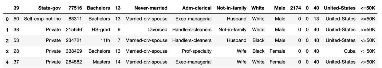
Figure 1.12 – The Census Income DataFrame
The output reveals that the column headings represent the entries of the first row. When this happens, the data may be reloaded with the header=None parameter:
df_census = pd.read_csv('https://archive.ics.uci.edu/ml/machine-learning-databases/adult/adult.data', header=None)
df_census.head()
Here is the expected output without the header:
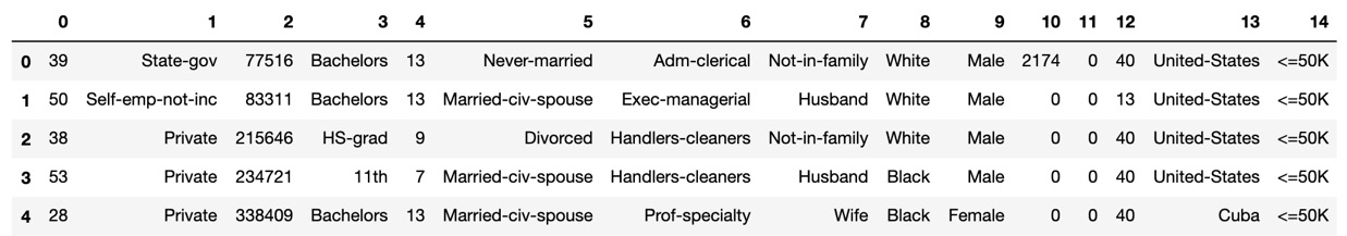
Figure 1.13 – The header=None parameter output
As you can see, the column names are still missing. They are listed on the Census Income Data Set website (https://archive.ics.uci.edu/ml/datasets/Census+Income) under Attribute Information.
Column names may be changed as follows:
df_census.columns=['age', 'workclass', 'fnlwgt', 'education', 'education-num', 'marital-status', 'occupation', 'relationship', 'race', 'sex', 'capital-gain', 'capital-loss', 'hours-per-week', 'native-country', 'income']
df_census.head()
Here is the expected output with column names:
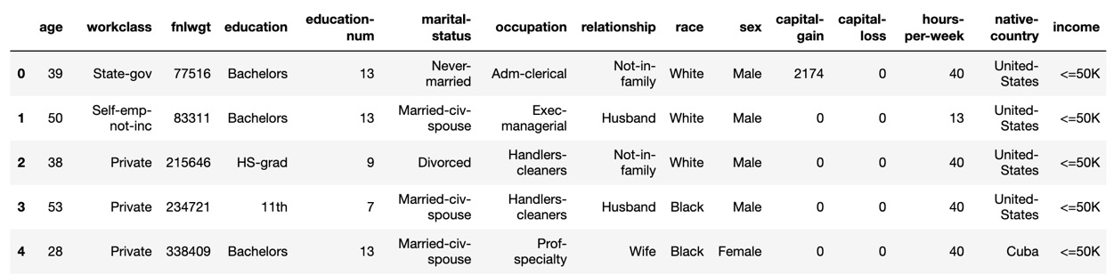
Figure 1.14 – Expected column names
As you can see, the column names have been restored.
Null values
A great way to check null values is to look at the DataFrame .info() method:
df_census.info()
The output is as follows:
<class 'pandas.core.frame.DataFrame'>
RangeIndex: 32561 entries, 0 to 32560
Data columns (total 15 columns):
 #   Column          Non-Null Count  Dtype
---  ------          --------------  -----
 0   age             32561 non-null  int64
 1   workclass       32561 non-null  object
 2   fnlwgt          32561 non-null  int64
 3   education       32561 non-null  object
 4   education-num   32561 non-null  int64
 5   marital-status  32561 non-null  object
 6   occupation      32561 non-null  object
 7   relationship    32561 non-null  object
 8   race            32561 non-null  object
 9   sex             32561 non-null  object
 10  capital-gain    32561 non-null  int64
 11  capital-loss    32561 non-null  int64
 12  hours-per-week  32561 non-null  int64
 13  native-country  32561 non-null  object
 14  income          32561 non-null  object
dtypes: int64(6), object(9)
memory usage: 3.7+ MB
Since all columns have the same number of non-null rows, we can infer that there are no null values.
Non-numerical columns
All columns of the dtype object must be transformed into numerical columns. A pandas get_dummies method takes the non-numerical unique values of every column and converts them into their own column, with 1 indicating presence and 0 indicating absence. For instance, if the column values of a DataFrame called "Book Types" were "hardback," "paperback," or "ebook," pd.get_dummies would create three new columns called "hardback," "paperback," and "ebook" replacing the "Book Types" column.
Here is a "Book Types" DataFrame:
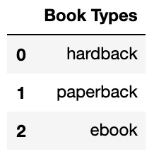
Figure 1.15 – A "Book Types" DataFrame
Here is the same DataFrame after pd.get_dummies:
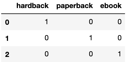
Figure 1.16 – The new DataFrame
pd.get_dummies will create many new columns, so it's worth checking to see whether any columns may be eliminated. A quick review of the df_census data reveals an 'education' column and an education_num column. The education_num column is a numerical conversion of 'education'. Since the information is the same, the 'education' column may be deleted:
df_census = df_census.drop(['education'], axis=1)
Now use pd.get_dummies to transform the non-numerical columns into numerical columns:
df_census = pd.get_dummies(df_census)
df_census.head()
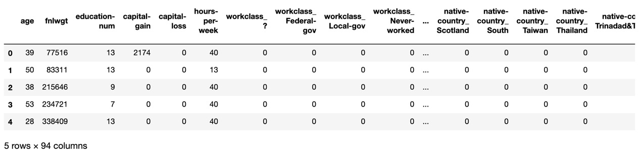
Figure 1.17 – pd.get_dummies – non-numerical to numerical columns
As you can see, new columns are created using a column_value syntax referencing the original column. For example, native-country is an original column, and Taiwan is one of many values. The new native-country_Taiwan column has a value of 1 if the person is from Taiwan and 0 otherwise.
Tip
Using pd.get_dummies may increase memory usage, as can be verified using the .info() method on the DataFrame in question and checking the last line. Sparse matrices may be used to save memory where only values of 1 are stored and values of 0 are not stored. For more information on sparse matrices, see Chapter 10, XGBoost Model Deployment, or visit SciPy's official documentation at https://docs.scipy.org/doc/scipy/reference/.
Target and predictor columns
Since all columns are numerical with no null values, it's time to split the data into target and predictor columns.
The target column is whether or not someone makes 50K. After pd.get_dummies, two columns, df_census['income_<=50K'] and df_census['income_>50K'], are used to determine whether someone makes 50K. Since either column will work, we delete df_census['income_ <=50K']:
df_census = df_census.drop('income_ <=50K', axis=1)
Now split the data into X (predictor columns) and y (target column). Note that -1 is used for indexing since the last column is the target column:
X = df_census.iloc[:,:-1]y = df_census.iloc[:,-1]
It's time to build machine learning classifiers!
Logistic regression
Logistic regression is the most fundamental classification algorithm. Mathematically, logistic regression works in a manner similar to linear regression. For each column, logistic regression finds an appropriate weight, or coefficient, that maximizes model accuracy. The primary difference is that instead of summing each term, as in linear regression, logistic regression uses the sigmoid function.
Here is the sigmoid function and the corresponding graph:
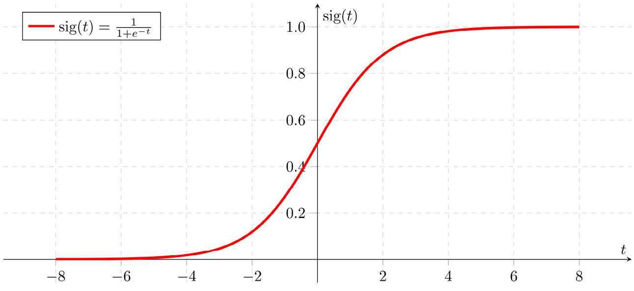
Figure 1.18 – Sigmoid function graph
The sigmoid is commonly used for classification. All values greater than 0.5 are matched to 1, and all values less than 0.5 are matched to 0.
Implementing logistic regression with scikit-learn is nearly the same as implementing linear regression. The main differences are that the predictor column should fit into categories, and the error should be in terms of accuracy. As a bonus, the error is in terms of accuracy by default, so explicit scoring parameters are not required.
You may import logistic regression as follows:
from sklearn.linear_model import LogisticRegression
The cross-validation function
Let's use cross-validation on logistic regression to predict whether someone makes over 50K.
Instead of copying and pasting, let's build a cross-validation classification function that takes a machine learning algorithm as input and has the accuracy score as output using cross_val_score:
def cross_val(classifier, num_splits=10): model = classifier scores = cross_val_score(model, X, y, cv=num_splits) print('Accuracy:', np.round(scores, 2)) print('Accuracy mean: %0.2f' % (scores.mean()))
Now call the function with logistic regression:
cross_val(LogisticRegression())
The output is as follows:
Accuracy: [0.8  0.8  0.79 0.8  0.79 0.81 0.79 0.79 0.8  0.8 ]
Accuracy mean: 0.80
80% accuracy isn't bad out of the box.
Let's see whether XGBoost can do better.
Tip
Any time you find yourself copying and pasting code, look for a better way! One aim of computer science is to avoid repetition. Writing your own data analysis and machine learning functions will make your life easier and your work more efficient in the long run.
The XGBoost classifier
XGBoost has a regressor and a classifier. To use the classifier, import the following algorithm:
from xgboost import XGBClassifier
Now run the classifier in the cross_val function with one important addition. Since there are 94 columns, and XGBoost is an ensemble method, meaning that it combines many models for each run, each of which includes 10 splits, we are going to limit n_estimators, the number of models, to 5. Normally, XGBoost is very fast. In fact, it has a reputation for being the fastest boosting ensemble method out there, a reputation that we will check in this book! For our initial purposes, however, 5 estimators, though not as robust as the default of 100, is sufficient. Details on choosing n_estimators will be a focal point of Chapter 4, From Gradient Boosting to XGBoost:
cross_val(XGBClassifier(n_estimators=5))
The output is as follows:
Accuracy: [0.85 0.86 0.87 0.85 0.86 0.86 0.86 0.87 0.86 0.86]
Accuracy mean: 0.86
As you can see, XGBoost scores higher than logistic regression out of the box.
Summary
Your journey through XGBoost has officially begun! You started this chapter by learning the fundamentals of data wrangling and pandas, essential skills for all machine learning practitioners, with a focus on correcting null values. Next, you learned how to build machine learning models in scikit-learn by comparing linear regression with XGBoost. Then, you prepared a dataset for classification and compared logistic regression with XGBoost. In both cases, XGBoost was the clear winner.
Congratulations on building your first XGBoost models! Your initiation into data wrangling and machine learning using the pandas, NumPy, and scikit-learn libraries is complete.
In Chapter 2, Decision Trees in Depth, you will improve your machine learning skills by building decision trees, the base learners of XGBoost machine learning models, and fine-tuning hyperparameters to improve results.