This chapter is about the Symbolic Aggregate Approximation (SAX) component of the iSAX index and is divided into two parts – the first part with the theoretical knowledge, and the second part with the code to compute SAX and the practical examples. At the end of the chapter, you will see how to calculate some handy statistical quantities that can give you a higher overview of your time series and plot a histogram of your data.

In this chapter, we will cover the following main topics:

• The required theory
• An introduction to SAX
• Developing a Python package
• Working with the SAX package
• Counting the SAX representations of a time series
• The tsfresh Python package
• Creating a histogram of a time series
• Calculating the percentiles of a time series

The GitHub repository for the book is https://github.com/PacktPublishing/Time-Series-Indexing. The code for each chapter is in its own directory. Therefore, the code for Chapter 2 can be found in the ch02 folder. If you already used git(1) to get a local copy of the entire GitHub repository, there is no need to get that again. Just make your current working directory ch02 while working with this chapter.

In this section, you are going to learn the required theory that supports the SAX representation. However, keep in mind that this book is more practical than it is theoretical. If you want to learn the theory in depth, you should read the research papers mentioned in this chapter, as well as the forthcoming ones, and the Useful links section found at the end of each chapter. Thus, the theory is about serving our main purpose, which is the implementation of techniques and algorithms.

The operation and the details of SAX are fully described in a research paper titled Experiencing SAX: a novel symbolic representation of time series, which was written by Jessica Lin, Eamonn Keogh, Li Wei, and Stefano Lonardi. This paper (https://doi.org/10.1007/s10618-007-0064-z) was officially published back in 2007. You do not have to read all of it from the front cover to the back cover, but it is a great idea to download it and read the first pages of it, giving special attention to the abstract and the introduction section.

We will begin by explaining the terms PAA and SAX. PAA stands for Piecewise Aggregate Approximation. The PAA representation offers a way to reduce the dimensionality of a time series. This means that it takes a long time series and creates a smaller version of it that is easier to work with.

PAA is also explained in the Experiencing SAX: a novel symbolic representation of time series paper (https://doi.org/10.1007/s10618-007-0064-z). From that, we can easily understand that PAA and SAX are closely related, as the idea behind SAX is based on PAA. The SAX representation is a symbolic representation of time series. Put simply, it offers a way of representing a time series in a summary form, in order to save space and increase speed.

The difference between PAA and SAX

The main difference between PAA and the SAX representation is that PAA just calculates the mean values of a time series, based on a sliding window size, whereas the SAX representation utilizes those mean values and further transforms PAA to get a discrete representation of a time series (or subsequence). In other words, the SAX representation converts the PAA representation into something that is better to work with. As you will find out in a while, this transformation takes place with the help of breakpoints, which divide the numeric space of the mean values into subspaces. Each subspace has a discrete representation based on the given breakpoint values.

Both PAA and SAX are techniques for dimensionality reduction. SAX is going to be explained in much more detail in a while, whereas the discussion about PAA ends here.

The next subsection tells us why we need SAX.

Why do we need SAX?

Time series are difficult to search. The longer a time series (or subsequence) is, the more computationally intensive it is to search for it or compare it with another one. The same applies to working with indexes that index time series – iSAX is such an index.

To make things simpler for you, what we will do is take a subsequence with x elements and transform it into a representation with w elements, where w is much smaller than x. In strict terms, this is called dimensionality reduction, and it allows us to work with long subsequences using less data. However, once we decide that we need to work with a given subsequence, we need to work with it using its full dimensions – that is, all its x elements.

The next subsection talks about normalization, which, among other things, allows us to compare values at different scales.

Normalization

The first two questions you might ask are what normalization is and why we need it.

Normalization is the process of adjusting values that use different scales to a common scale. A simple example is comparing Fahrenheit and Celsius temperatures – we cannot do that unless we bring all values to the same scale. This is the simplest form of normalization.

Although various types of normalization exist, what is needed here is standard score normalization, which is the simplest form of normalization, because this is what is used for time series and subsequences. Please do not confuse database normalization and normal forms with value normalization, as they are totally different concepts.

The reasons that we introduce normalization into the process are as follows:

• The first and most important reason is that we can compare datasets that use a different range of values. A simple case is comparing Celsius and Fahrenheit temperatures.
• A side effect of the previous point is that data anomalies are reduced but not eliminated.
• In general, normalized data is easier to understand and process because we deal with values in a predefined range.
• Searching using an index that uses normalized values might be faster than when working with bigger values.
• Searching, sorting, and creating indexes is faster since values are smaller.
• Normalization is conceptually cleaner and easier to maintain and change as your needs change.

Another simple example that supports the need for normalization is when comparing positive values with negative ones. It is almost impossible to draw useful conclusions when comparing such different kinds of observations. Normalization solves such issues.

Although we are not going to need to, bear in mind that we cannot go from the normalized version of a subsequence to the original subsequence, so the normalization process is irreversible.

The following function shows how to normalize a time series with some help from the NumPy Python package:

def normalize(x):
     eps = 1e-6
     mu = np.mean(x)
     std = np.std(x)
     if std < eps:
           return np.zeros(shape=x.shape)
     else:
           return (x-mu)/std

The previous function reveals the formula of normalization. Given a dataset, the normalized form of each one of its elements is equal to the value of the observation, minus the mean value of the dataset over the standard deviation of the dataset – both these statistical terms are explained in The tsfresh Python package section of this chapter.

This is seen in the return value of the previous function, (x-mu)/std. NumPy is clever enough to calculate that value for each observation without the need to use a for loop. If the standard deviation is close to 0, which is simulated by the value of the eps variable, then the return value of normalize() is equal to a NumPy array full of zeros.

The normalize.py script, which uses the previously developed function that does not appear here, gets a time series as input and returns its normalized version. Its code is as follows:

#!/usr/bin/env python3
import sys
import pandas as pd
import numpy as np
def main():
     if len(sys.argv) != 2:
           print("TS")
           sys.exit()
     F = sys.argv[1]
     ts = pd.read_csv(F, compression='gzip', header = None)
     ta = ts.to_numpy()
     ta = ta.reshape(len(ta))
     taNorm = normalize(ta)
     print("[", end = ' ')
     for i in taNorm.tolist():
           print("%.4f" % i, end = ' ')
     print("]")
if __name__ == '__main__':
     main()

The last for loop of the program is used to print the contents of the taNorm NumPy array with a smaller precision in order to take up less space. To do that, we need to convert the taNorm NumPy array into a regular Python list using the tolist() method.

We are going to feed normalize.py a short time series; however, the script also works with longer ones. The output of normalize.py looks as follows:

$ ./normalize.py ts1.gz
[ -1.2272 0.9487 -0.1615 -1.0444 -1.3362 1.4861 -1.0620 0.7451 -0.4858 -0.9965 0.0418 1.7273 -1.1343 0.6263 0.3455 0.9238 1.2197 0.3875 -0.0483 -1.7054 1.3272 1.5999 1.4479 -0.4033 0.1525 1.0673 0.7019 -1.0114 0.4473 -0.2815 1.1239 0.7516 -1.3102 -0.6428 -0.3186 -0.3670 -1.6163 -1.2383 0.5692 1.2341 -0.0372 1.3250 -0.9227 0.2945 -0.5290 -0.3187 1.4103 -1.3385 -1.1540 -1.2135 ]

With normalization in mind, let us now proceed to the next subsection, where we are going to visualize a time series and show the visual difference between the original version and the normalized version of it.

Visualizing normalized time series

In this subsection, we are going to show the difference between the normalized and the original version of a time series with the help of visualization. Keep in mind that we usually do not normalize the entire time series. The normalization takes place on a subsequence level based on the sliding window size. In other words, for the purposes of this book, we will normalize subsequences, not an entire time series. Additionally, for the calculation of the SAX representation, we process the normalized subsequences based on the segment value, which specifies the parts that a SAX representation will have. So, for a segment value of 2, we split the normalized subsequence into two. For a segment value of 4, we split the normalized subsequence into four sets.

Nevertheless, viewing the normalized and original versions of a time series is very educational. The Python code of visualize_normalized.py, without the implementation of normalize(), is as follows:

#!/usr/bin/env python3
import sys
import pandas as pd
import matplotlib.pyplot as plt
import numpy as np
def main():
     if len(sys.argv) != 2:
           print("TS")
           sys.exit()
     F = sys.argv[1]
     ts = pd.read_csv(F, compression='gzip', header = None)
     ta = ts.to_numpy()
     ta = ta.reshape(len(ta))
     # Find its normalized version
     taNorm = normalize(ta)
     plt.plot(ta, label="Regular", linestyle='-', markevery=10, marker='o')
     plt.plot(taNorm, label="Normalized", linestyle='-.', markevery=10, marker='o')
     plt.xlabel('Time Series', fontsize=14)
     plt.ylabel('Values', fontsize=14)
     plt.legend()
     plt.grid()
     plt.savefig("CH02_01.png", dpi=300, format='png', bbox_inches='tight')
if __name__ == '__main__':
     main()

The plt.plot() function is called twice, plotting a line each time. Feel free to experiment with the Python code in order to change the look of the output.

Figure 2.1 shows the output of visualize_normalized.py ts1.gz, which uses a time series with 50 elements.

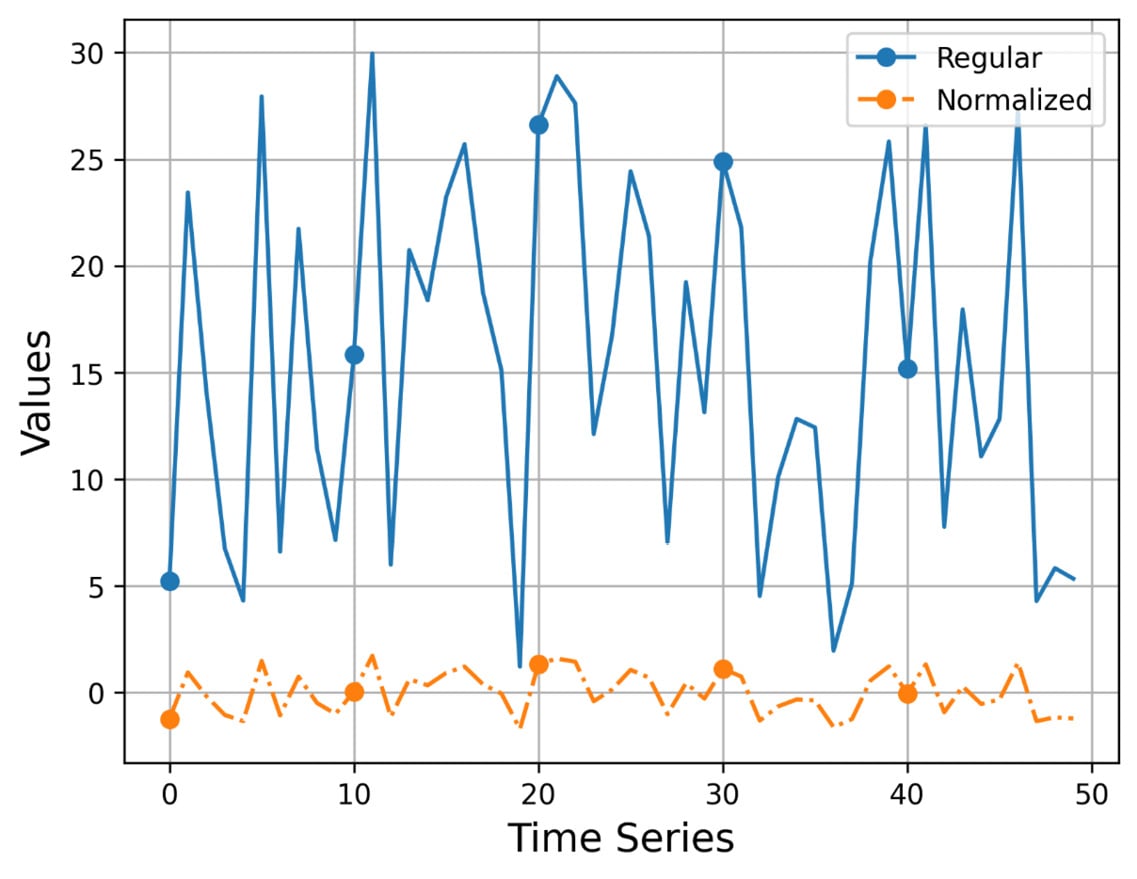
Figure 2.1 – The plotting of a time series and its normalized version

I think that Figure 2.1 speaks for itself! The values of the normalized version are located around the value of 0, whereas the values of the original time series can be anywhere! Additionally, we make the original time series smoother without completely losing its original shape and edges.

The next section is about the details of the SAX representation, which is a key component of every iSAX index.

As mentioned previously, SAX stands for Symbolic Aggregate Approximation. The SAX representation was officially announced back in 2007 in the Experiencing SAX: a novel symbolic representation of time series paper (https://doi.org/10.1007/s10618-007-0064-z).

Keep in mind that we do not want to find the SAX representation of an entire time series. We just want to find the SAX representation of a subsequence of a time series. The main difference between a time series and a subsequence is that a time series is many times bigger than a subsequence.

Each SAX representation has two parameters named cardinality and the number of segments. We will begin by explaining the cardinality parameter.

The cardinality parameter

The cardinality parameter specifies the number of possible values each segment can have. As a side effect, the cardinality parameter defines the way the y axis is divided – this is used to get the value of each segment. There exist multiple ways to specify the value of a segment based on the cardinality. These include alphabet characters, decimal numbers, and binary numbers. In this book, we will use binary numbers because they are easier to understand and interpret, using a file with the precalculated breakpoints for cardinalities up to 256.

So, a cardinality of 4, which is 22, gives us four possible values, as we use 2 bits. However, we can easily replace 00 with the letter a, 01 with the letter b, 10 with the letter c, 11 with the letter d, and so on, in order to use letters instead of binary numbers. Keep in mind that this might require minimal code changes in the presented code, and it would be good to try this as an exercise when you feel comfortable with SAX and the provided Python code.

The format of the file with the breakpoints, which in our case supports cardinalities up to 256 and is called SAXalphabet, is as follows:

$ head -7 SAXalphabet
0
-0.43073,0.43073
-0.67449,0,0.67449
-0.84162,-0.25335,0.25335,0.84162
-0.96742,-0.43073,0,0.43073,0.96742
-1.0676,-0.56595,-0.18001,0.18001,0.56595,1.0676
-1.1503,-0.67449,-0.31864,0,0.31864,0.67449,1.1503

The values presented here are called breakpoints in the SAX terminology. The value in the first line divides the y axis into two areas, separated by the x axis. So, in this case, we need 1 bit to define whether we are in the upper space (the positive y value) or the lower one (the negative y value).

As we will use binary numbers to represent each SAX segment, there is no point in wasting them. Therefore, the values that we will use are the powers of 2, from 2 1 (cardinality 2) to 2 8 (cardinality 256).

Let us now present Figure 2.2, which shows how -0.67449, 0, 0.67449 divides the y axis, which is used in the 2 2 cardinality. The bottom part begins from the minus infinitive up to -0.67449, the second part from -0.67449 up to 0, the third part from 0 to 0.67449, and the last part from 0.67449 up to plus infinitive.

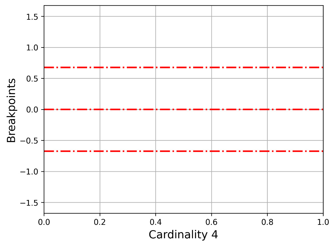
Figure 2.2 – The y axis for cardinality 4 (three breakpoints)

Let us now present Figure 2.3, which shows how -1.1503, -0.67449, -0.31864, 0, 0.31864, 0.67449, 1.1503 divides the y axis. This is for the 2 3 cardinality.

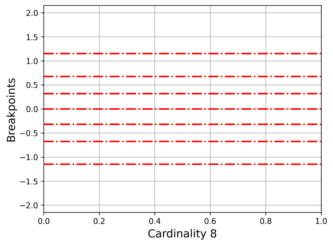
Figure 2.3 – The y axis for cardinality 8 (7 breakpoints)

As this can be a tedious job, we have created a utility that does all the plotting. Its name is cardinality.py, and it reads the SAXalphabet file to find the breakpoints of the desired cardinality before plotting them.

The Python code for cardinality.py is as follows:

#!/usr/bin/env python3
import sys
import pandas as pd
import matplotlib.pyplot as plt
import numpy as np
import os
breakpointsFile = "./sax/SAXalphabet"
def main():
     if len(sys.argv) != 3:
           print("cardinality output")
           sys.exit()
     n = int(sys.argv[1]) - 1
     output = sys.argv[2]
     path = os.path.dirname(__file__)
     file_variable = open(path + "/" + breakpointsFile)
     alphabet = file_variable.readlines()
     myLine = alphabet[n - 1].rstrip()
     elements = myLine.split(',')
     lines = [eval(i) for i in elements]
     minValue = min(lines) - 1
     maxValue = max(lines) + 1
     fig, ax = plt.subplots()
     for i in lines:
           plt.axhline(y=i, color='r', linestyle='-.', linewidth=2)
     xLabel = "Cardinality " + str(n)
     ax.set_ylim(minValue, maxValue)
     ax.set_xlabel(xLabel, fontsize=14)
     ax.set_ylabel('Breakpoints', fontsize=14)
     ax.grid()
     fig.savefig(output, dpi=300, format='png', bbox_inches='tight')
if __name__ == '__main__':
     main()

The script requires two command-line parameters – the cardinality and the output file, which is used to save the image. Note that a cardinality value of 8 requires 7 breakpoints, a cardinality value of 32 requires 31 breakpoints, and so on. Therefore, the Python code for cardinality.py decreases the line number that it is going to search for in the SAXalphabet file to support that functionality. Therefore, when given a cardinality value of 8, the script is going to look for the line with 7 breakpoints in SAXalphabet. Additionally, as the script reads the breakpoint values as strings, we need to convert these strings into floating-point values using the lines = [eval(i) for i in elements] statement. The rest of the code is related to the Matplotlib Python package and how to draw lines using plt.axhline().

The next subsection is about the segments parameter.

The segments parameter

The (number of) segments parameter specifies the number of parts (words) a SAX representation is going to have. Therefore, a segments value of 2 means that the SAX representation is going to have two words, each one using the specified cardinality. Therefore, the values of each part are determined by the cardinality.

A side effect of this parameter is that, after normalizing a subsequence, we divide it by the number of segments and work with these different parts separately. This is the way the SAX representation works.

Both cardinality and segments values control the data compression ratio and the accuracy of the subsequences of a time series and, therefore, the entire time series.

The next subsection shows how to manually compute the SAX representation of a subsequence – this is the best way to fully understand the process and be able to identify bugs or errors in the code.

How to manually find the SAX representation of a subsequence

Finding the SAX representation of a subsequence looks easy but requires lots of computations, which makes the process ideal for a computer. Here are the steps to find the SAX representation of a time series or subsequence:

1. First, we need to have the number of segments and the cardinality.
2. Then, we normalize the subsequence or the time series.
3. After that, we divide the normalized subsequence by the number of segments.
4. For each one of these parts, we find its mean value.
5. Finally, based on each mean value, we calculate its representation based on the cardinality. The cardinality is what defines the breakpoint values that are going to be used.

We will use two simple examples to illustrate the manual computation of the SAX representation of a time series. The time series is the same in both cases. What will be different are the SAX parameters and the sliding window size.

Let’s imagine we have the following time series and a sliding window size of 4:

{-1, 2, 3, 4, 5, -1, -3, 4, 10, 11, . . .}

Based on the sliding window size, we extract the first two subsequences from the time series:

• S1 = {-1, 2, 3, 4}
• S2 = {2, 3, 4, 5}

The first step that we should take is to normalize these two subsequences. For that, we will use the normalize.py script we developed earlier – we just have to save each subsequence into its own plain text file and compress it using the gzip utility, before giving it as input to normalize.py. If you use a Microsoft Windows machine, you should look for a utility that allows you to create such ZIP files. An alternative is to work with plain text files, which might require some small code changes in the pd.read_csv() function call.

The output of the normalize.py script when processing S1 (s1.txt.gz) and S2 (s2.txt.gz) is the following:

$ ./normalize.py s1.txt.gz
[ -1.6036 0.0000 0.5345 1.0690 ]
$ ./normalize.py s2.txt.gz
[ -1.3416 -0.4472 0.4472 1.3416 ]

So, the normalized versions of S1 and S2 are as follows:

• N1 = {-1.6036, 0.0000, 0.5345, 1.0690}
• N2 = {-1.3416, -0.4472, 0.4472, 1.3416}

In this first example, we use a segments value of 2 and a cardinality value of 4 (22). A segment value of 2 means that we must divide each normalized subsequence into two parts. These two parts contain the following data, based on the normalized versions of S1 and S2:

• For S1, the two parts are {-1.6036, 0.0000} and {0.5345, 1.0690}
• For S2, the two parts are {-1.3416, -0.4472} and {0.4472, 1.3416}

The mean values of each part are as follows:

• For S1, they are -0.8018 and 0.80175
• For S2, they are -0.8944 and 0.8944

For the cardinality of 4, we are going to look at Figure 2.2 and the respective breakpoints, which are -0.67449, 0, and 0.67449. So, the SAX values of each segment are as follows:

• For S1, they are 00 because -0.8018 falls at the bottom of the plot and 11
• For S2, they are 00 and 11 because 0.8944 falls at the top of the plot

Therefore, the SAX representation of S1 is [00, 11] and for S2, it is [00, 11]. It turns out that both subsequences have the same SAX representation. This makes sense, as they only differ in one element, which means that their normalized versions are similar.

Note that in both cases, the lower cardinality begins from the bottom of the plot. For Figure 2.2, this means that 00 is at the bottom of the plot, 01 is next, followed by 10, and 11 is at the top of the plot.

In the second example, we will use a sliding window size of 8, a segments value of 4, and a cardinality value of 8 (23).

About the sliding window size

Keep in mind that the normalized representation of the subsequence remains the same when the sliding window size remains the same. However, if either the cardinality or the segments change, the resulting SAX representation might be completely different.

Based on the sliding window size, we extract the first two subsequences from the time series – S1 = {-1, 2, 3, 4, 5, -1, -3, 4} and S2 = {2, 3, 4, 5, -1, -3, 4, 10}.

The output of the normalize.py script is going to be the following:

$ ./normalize.py T1.txt.gz
[ -0.9595 0.1371 0.5026 0.8681 1.2337 -0.9595 -1.6906 0.8681 ]
$ ./normalize.py T2.txt.gz
[ -0.2722 0.0000 0.2722 0.5443 -1.0887 -1.6330 0.2722 1.9052 ]

So, the normalized versions of S1 and S2 are N1 = {-0.9595, 0.1371, 0.5026, 0.8681, 1.2337, -0.9595, -1.6906, 0.8681} and N2 = {-0.2722, 0.0000, 0.2722, 0.5443, -1.0887, -1.6330, 0.2722, 1.9052}, respectively.

A segment value of 4 means that we must divide each one of the normalized subsequences into four parts. For S1, these parts are {-0.9595, 0.1371}, {0.5026, 0.8681}, {1.2337, -0.9595}, and {-1.6906, 0.8681}.

For S2, these parts are {-0.2722, 0.0000}, {0.2722, 0.5443}, {-1.0887, -1.6330}, and {0.2722, 1.9052}.

For S1, the mean values are -0.4112, 0.68535, 0.1371, and -0.41125. For S2, the mean values are -0.1361, 0.40825, -1.36085, and 1.0887.

About the breakpoints of the cardinality value of 8

Just a reminder here that for the cardinality value of 8, the breakpoints are (000) -1.1503, (001) -0.67449, (010) -0.31864, (011) 0, (100) 0.31864, (101) 0.67449, and (110) 1.1503 (111). In parentheses, we present the SAX values for each breakpoint. For the first breakpoint, we have the 000 value to its left and 001 to its right. For the last breakpoint, we have the 110 value to its left and 111 to its right. Remember that we use seven breakpoints for a cardinality value of 8.

Therefore, the SAX representation of S1 is ['010', '110', '100', '010'], and for S2, it is['011', '101', '000', '110']. The use of single quotes around SAX words means that internally we store SAX words as strings, despite the fact that we calculate them as binary numbers because it is easier to search and compare strings.

The next subsection examines a case where a subsequence cannot be divided perfectly by the number of segments.

Ηow can we divide 10 data points into 3 segments?

So far, we have seen examples where the length of the subsequence can be perfectly divided by the number of segments. However, what happens if that is not possible?

In that case, there exist data points that contribute to two adjacent segments at the same time. However, instead of putting the whole point into a segment, we put part of it into one segment and part of it into another!

This is further explained on page 18 of the Experiencing SAX: a novel symbolic representation of time series paper. As stated in the paper, if we cannot divide the sliding window length by the number of segments, we can use a part of a point in a segment and a part of a point in another segment. We do that for points that are between two segments and not for any random points. This can be explained using an example. Imagine we have a time series such as T = {t1, t2, t3, t4, t5, t6, t7, t8, t9, t10}. For the S1 segment, we take the values of {t1, t2, t3} and one-third of the value of t4. For the S2 segment, we take the values of {t5, t6} and two-thirds of the values of t4 and t7. For the S3 segment, we take the values of {t8, t9, t10} and the third of the value of t7 that we have not used so far. This is also explained in Figure 2.4:

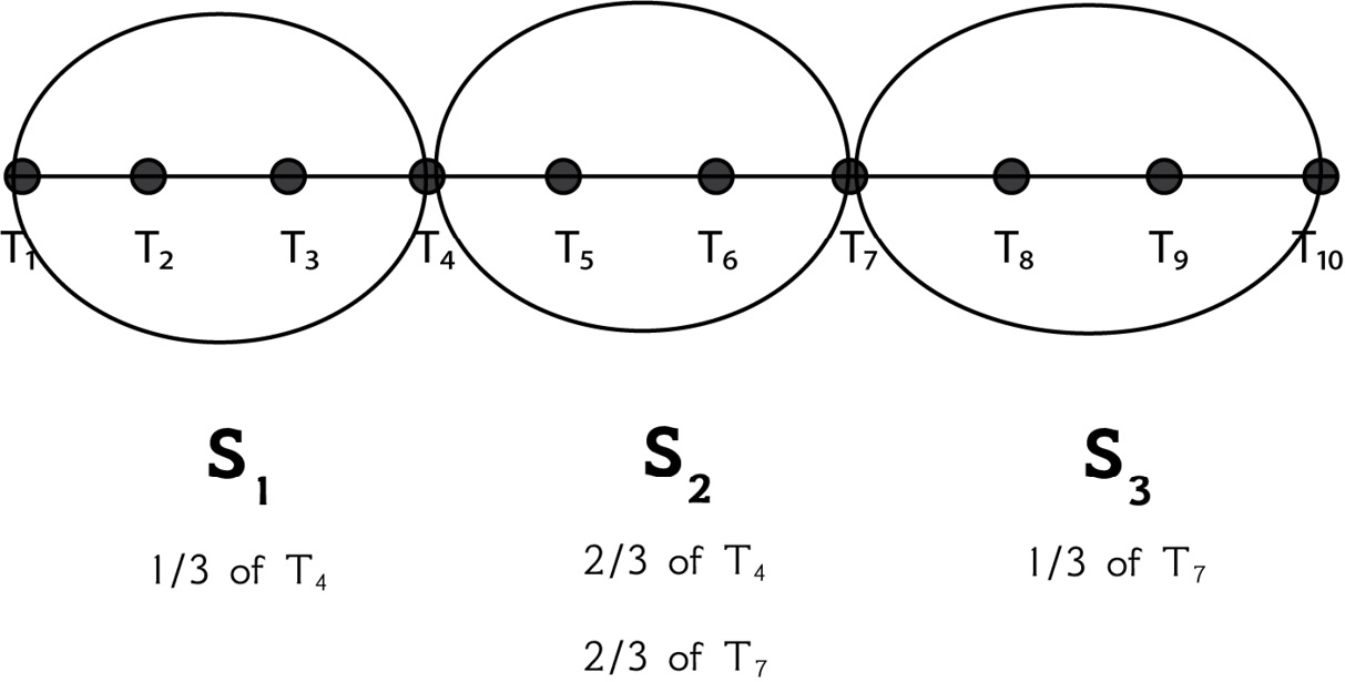
Figure 2.4 – Dividing 10 data points into 3 segments

Put simply, this is a convention decided by the creators of SAX that applies to all cases where we cannot perfectly divide the number of elements by that of the segments.

In this book, we will not deal with that case. The sliding window size, which is the length of the generated subsequences, and the number of segments are both part of a perfect division, with a remainder of 0. This simplification does not change the way SAX works, but it makes our lives a little easier.

The subject of the next subsection is how to go from higher cardinalities to lower ones without doing every computation.

Reducing the cardinality of a SAX representation

The knowledge gained from this subsection will be applicable when we discuss the iSAX index. However, as what you will learn is directly related to SAX, we have decided to discuss it here first.

Imagine that we have a SAX representation at a given cardinality and that we want to reduce the cardinality. Is that possible? Can we do this without calculating everything from scratch? The answer is simple – this can be done by ignoring trailing bits. Given a binary value of 10,100, the first trailing bit is 0, then the next trailing bit is 0, then 1, and so on. So, we start from the bits at the end, and we remove them one by one.

As most of you, including me when I first read about it, might find this unclear, let me show you some practical examples. Let us take the following two SAX representations from the How to manually find the SAX representation of a subsequence subsection of this chapter – [00, 11] and [010, 110, 100, 010]. To convert [00, 11] into the cardinality of 2, we must just delete the digits at the end of each SAX word. So, the new version of [00, 11] will be [0, 1]. Similarly, [010, 110, 100, 010] is going to be [01, 11, 10, 01] for the cardinality of 4 and [0, 1, 1, 0] for the cardinality of 2.

So, from a higher cardinality – a cardinality with more digits – we can go to a lower cardinality by subtracting the appropriate number of digits from the right side of one or more segments (the trailing bits). Can we go in the opposite direction? Not without losing accuracy, but that would still be better than nothing. However, generally, we don’t go in the opposite direction. So far, we know the theory regarding the SAX representation. The section that follows briefly explains the basics of Python packages and shows the development of our own package, named sax.

In this section, we describe the process of developing a Python package that calculates the SAX representation of a subsequence. Apart from this being a good programming exercise, the package is going to be enriched in the chapters that follow when we create the iSAX index.

We will begin by explaining the basics of Python packages.

The basics of Python packages

I am not a Python expert, and the presented information is far from complete. However, it covers the required knowledge regarding Python packages.

In all but the latest Python versions, we used to need a file named __init__.py inside the directory of every Python package. Its purpose is to perform initialization actions and imports, as well as define variables. Although this is not the case with most recent Python versions, our packages will still have a __init__.py file in them. The good thing is that it is allowed to be empty if you have nothing to put into it. There is a link at the end of the chapter to the official Python documentation regarding packages, regular packages, and namespace packages, where the use of __init__.py is explained in more detail.

The next subsection discusses the details of the Python package that we are going to develop.

The SAX Python package

The code of the sax Python package is included in a directory named sax. The contents of the sax directory are presented with the help of the tree(1) command, which you might need to install on your own:

$ tree sax
sax
├── SAXalphabet
├── __init__.py
├── __pycache__
│   __init__.cpython-310.pyc
│   sax.cpython-310.pyc
│   tools.cpython-310.pyc
│   variables.cpython-310.pyc
├── sax.py
├── tools.py
└── variables.py
2 directories, 9 files

The __pycache__ directory is automatically generated by Python once you begin using the Python package and contains precompiled bytecode Python code. You can completely ignore that directory.

Let us begin by showing the contents of sax.py, which is going to be presented in multiple code chunks.

First, we have the import section and the implementation of the normalize() function, which normalizes a NumPy array:

import numpy as np
from scipy.stats import norm
from sax import tools
import sys
sys.path.insert(0,'..')
def normalize(x):
     eps = 1e-6
     mu = np.mean(x)
     std = np.std(x)
     if std < eps:
           return np.zeros(shape=x.shape)
     else:
           return (x-mu)/std

After that, we have the implementation of the createPAA() function, which returns the SAX representation of a time series, given the cardinality and the segments:

def createPAA(ts, cardinality, segments):
     SAXword = ""
     ts_norm = normalize(ts)
     segment_size = len(ts_norm) // segments
     mValue = 0
     for I in range(segments):
           ts_segment = ts_norm[segment_size * i :(i+1) * segment_size]
           mValue = meanValue(ts_segment)
           index = getIndex(mValue, cardinality)
           SAXword += str(index) +""""

Python uses the double slash // operator to perform floor division. What the // operator does is divide the first number by the second number before rounding the result down to the nearest integer – this is used for the segment_size variable.

The rest of the code is about specifying the correct index numbers when working with the given time series (or subsequence). Hence, the for loop is used to process the entire time series (or subsequence) based on the segments value.

Next, we have the implementation of a function that computes the mean value of a NumPy array:

def meanValue(ts_segment):
     sum = 0
     for i in range(len(ts_segment)):
           sum += ts_segment[i]
     mean_value = sum / len(ts_segment)
     return mean_value

Finally, we have the function that returns the SAX value of a SAX word, given its mean value and its cardinality. Remember that we calculate the mean value of each SAX word separately in the createPAA() function:

def getIndex(mValue, cardinality):
     index = 0
     # With cardinality we get cardinality + 1
     bPoints = tools.breakpoints(cardinality-1)
     while mValue < float(bPoints[index]):
           if index == len(bPoints)–- 1:
                 # This means that index should be advanced
                 # before breaking out of the while loop
                 index += 1
                 break
           else:
                 index += 1
     digits = tools.power_of_two(cardinality)
     # Inverse the result
     inverse_s = ""
     for i in binary_index:
           if i == '0':
                 inverse_s += '1'
           else:
                 inverse_s += '0'
     return inverse_s

The previous code computes the SAX value of a SAX word using its mean value. It iteratively visits the breakpoints, from the lowest value to the biggest, up to the point that the mean value exceeds the current breakpoint. This way, we find the index of the SAX word (mean value) in the list of breakpoints.

Now, let us discuss a tricky point, which has to do with the last statements that reverse the SAX word. This mainly has to do with whether we begin counting from the top or the bottom of the different areas that the breakpoints create. All ways are equivalent – we just decided to go that way. This is because a previous implementation of SAX used that order, and we wanted to make sure that we created the same results for testing reasons. If you want to alter that functionality, you just have to remove the last for loop.

As you saw at the beginning of this section, the sax package is composed of three Python files, not just the one that we just presented. So, we will present the remaining two files.

First, we will present the contents of variables.py:

# This file includes all variables for the sax package
maximumCardinality = 32
# Where to find the breakpoints file
# In this case, in the current directory
breakpointsFile =""SAXalphabe""
# Sliding window size
slidingWindowSize = 16
# Segments
segments = 0
# Breakpoints in breakpointsFile
elements ="""
# Floating point precision
precision = 5

You might wonder what the main reason is for having such a file. The answer is that we need to have a place to keep our global parameters and options, and having a separate file for that is a perfect solution. This will make much more sense when the code becomes longer and more complex.

Second, we present the code in tools.py:

import os
import numpy as np
import sys
from sax import variables
breakpointsFile = variables.breakpointsFile
maxCard = variables.maximumCardinality

Here, we reference two variables from the variable.py file, which are variables.breakpointsFile and variables.maximumCardinality:

def power_of_two(n):
     power = 1
     while n/2 != 1:
           # Not a power of 2
           if n % 2 == 1:
                 return -1
           n = n / 2
           power += 1
     return power

This is a helper function that we use when we want to make sure that a value is a power of 2:

def load_sax_alphabet():
     path = os.path.dirname(__file__)
     file_variable = open(path +"""" + breakpointsFile)
     variables.elements = file_variable.readlines()
def breakpoints(cardinality):
     if variables.elements ==""":
           load_sax_alphabet()
     myLine = variables.elements[cardinality–- 1].rstrip()
     elements = myLine.split'''')
     elements.reverse()
     return elements

The load_sax_alphabet() function loads the contents of the file with the definitions of breakpoints and assigns them to the variables.elements variable. The breakpoints() function returns the breakpoint values when given the cardinality.

As you can see, the code of the entire package is relatively short, which is a good thing.

In this section, we developed a Python package to compute SAX representations. In the next section, we are going to begin working with the sax package.

Now that we have the SAX package at hand, it is time to use it by developing various utilities, starting with a utility that computes the SAX representations of the subsequences of a time series.

Computing the SAX representations of the subsequences of a time series

In this subsection, we will develop a utility that computes the SAX representations for all the subsequences of a time series and also presents their normalized forms. The name of the utility is ts2PAA.py and contains the following code:

#!/usr/bin/env python3
import sys
import numpy as np
import pandas as pd
from sax import sax
def main():
     if len(sys.argv) != 5:
           print("TS1 sliding_window cardinality segments")
           sys.exit()
     file = sys.argv[1]
     sliding = int(sys.argv[2])
     cardinality = int(sys.argv[3])
     segments = int(sys.argv[4])
     if sliding % segments != 0:
           print("sliding MODULO segments != 0...")
           sys.exit()
     if sliding <= 0:
           print("Sliding value is not allowed:", sliding)
           sys.exit()
     if cardinality <= 0:
           print("Cardinality Value is not allowed:", cardinality)
           sys.exit()
     # Read Sequence as Pandas
     ts = pd.read_csv(file, names=['values'], compression='gzip')
     # Convert to NParray
     ts_numpy = ts.to_numpy()
     length = len(ts_numpy)
     PAA_representations = []
     # Split sequence into subsequences
     for i in range(length - sliding + 1):
           t1_temp = ts_numpy[i:i+sliding]
           # Generate SAX for each subsequence
           tempSAXword = sax.createPAA(t1_temp, cardinality, segments)
           SAXword = tempSAXword.split("_")[:-1]
           print(SAXword, end = ' ')
           PAA_representations.append(SAXword)
           print("[", end = ' ')
           for i in t1_temp.tolist():
                 for k in i:
                       print("%.2f" % k, end = ' ')
           print("]", end = ' ')
           print("[", end = ' ')
           for i in sax.normalize(t1_temp).tolist():
                 for k in i:
                       print("%.2f" % k, end = ' ')
           print("]")
if __name__ == '__main__':
     main()

The ts2PAA.py script takes a time series, breaks it into subsequences, and computes the normalized version of each subsequence using sax.normalize().

The output of ts2PAA.py is as follows (some output is omitted for brevity):

$ ./ts2PAA.py ts1.gz 8 4 2
['01', '10'] [ 5.22 23.44 14.14 6.75 4.31 27.94 6.61 21.73 ] [ -0.97 1.10 0.04 -0.80 -1.07 1.61 -0.81 0.90 ]
['01', '10'] [ 23.44 14.14 6.75 4.31 27.94 6.61 21.73 11.43 ] [ 1.07 -0.05 -0.94 -1.24 1.62 -0.96 0.87 -0.38 ]
['10', '01'] [ 14.14 6.75 4.31 27.94 6.61 21.73 11.43 7.15 ] [ 0.21 -0.73 -1.05 1.97 -0.75 1.18 -0.14 -0.68 ]
['01', '10'] [ 6.75 4.31 27.94 6.61 21.73 11.43 7.15 15.85 ] [ -0.76 -1.07 1.93 -0.77 1.14 -0.16 -0.70 0.40 ]
['01', '10'] [ 4.31 27.94 6.61 21.73 11.43 7.15 15.85 29.96 ] [ -1.22 1.32 -0.97 0.66 -0.45 -0.91 0.02 1.54 ]
['10', '01'] [ 27.94 6.61 21.73 11.43 7.15 15.85 29.96 6.00 ] [ 1.34 -1.02 0.65 -0.49 -0.96 0.00 1.56 -1.08 ]
. . .

The previous output shows the SAX representation, the original subsequence, and the normalized version of the subsequence for all the subsequences of a time series. Each subsequence is on a separate line.

Using Python packages

Most of the chapters that follow will need the SAX package we developed here. For reasons of simplicity, we will copy the SAX package implementation into all directories that use that package. This might not be the best practice on production systems where we want a single copy of each software or package, but it is the best practice when learning and experimenting.

So far, we have learned how to use the basic functionality of the sax package.

The next section presents a utility that counts the SAX representations of the subsequences of a time series and prints the results.

This section of the chapter presents a utility that counts the SAX representations of a time series. The Python data structure behind the logic of the utility is a dictionary, where the keys are the SAX representations converted into strings and the values are integers.

The code for counting.py is as follows:

#!/usr/bin/env python3
import sys
import pandas as pd
from sax import sax
def main():
     if len(sys.argv) != 5:
           print("TS1 sliding_window cardinality segments")
           print("Suggestion: The window be a power of 2.")
           print("The cardinality SHOULD be a power of 2.")
           sys.exit()
     file = sys.argv[1]
     sliding = int(sys.argv[2])
     cardinality = int(sys.argv[3])
     segments = int(sys.argv[4])
     if sliding % segments != 0:
           print("sliding MODULO segments != 0...")
           sys.exit()
     if sliding <= 0:
           print("Sliding value is not allowed:", sliding)
           sys.exit()
     if cardinality <= 0:
           print("Cardinality Value is not allowed:", cardinality)
           sys.exit()
     ts = pd.read_csv(file, names=['values'], compression='gzip')
     ts_numpy = ts.to_numpy()
     length = len(ts_numpy)
     KEYS = {}
     for i in range(length - sliding + 1):
           t1_temp = ts_numpy[i:i+sliding]
           # Generate SAX for each subsequence
           tempSAXword = sax.createPAA(t1_temp, cardinality, segments)
           tempSAXword = tempSAXword[:-1]
           if KEYS.get(tempSAXword) == None:
                 KEYS[tempSAXword] = 1
           else:
                 KEYS[tempSAXword] = KEYS[tempSAXword] + 1
     for k in KEYS.keys():
           print(k, ":", KEYS[k])
if __name__ == '__main__':
     main()

The for loop splits the time series into subsequences and computes the SAX representation of each subsequence using sax.createPAA(), before updating the relevant counter in the KEYS dictionary. The tempSAXword = tempSAXword[:-1] statement removes an unneeded underscore character from the SAX representation. Finally, we print the content of the KEYS dictionary.

The output of counting.py should be similar to the following:

$ ./counting.py ts1.gz 4 4 2
10_01 : 18
11_00 : 8
01_10 : 14
00_11 : 7

What does this output tell us?

For a time series with 50 elements (ts1.gz) and a sliding window size of 4, there exist 18 subsequences with the 10_01 SAX representation, 8 subsequences with the 11_00 SAX representation, 14 subsequences with the 01_10 SAX representation, and 7 subsequences with the 00_11 SAX representation. For easier comparison, and to be able to use a SAX representation as a key to a dictionary, we convert [01 10] into the 01_10 string, [11 00] into 11_00, and so on.

How many subsequences does a time series have?

Keep in mind that given a time series with n elements and a sliding window size of w, the total number of subsequences is n – w + 1.

counting.py can be used for many practical tasks and will be updated in Chapter 3.

The next section discusses a handy Python package that can help us learn more about processing our time series from a statistical point of view.

This is a bonus section not directly related to the subject of the book, but it is helpful, nonetheless. It is about a handy Python package called tsfresh, which can give you a good overview of your time series from a statistical perspective. We are not going to present all the capabilities of tsfresh, just the ones that you can easily use to get information about your time series data – at this point, you might need to install tsfresh on your machine. Keep in mind that the tsfresh package has lots of package dependencies.

So, we are going to compute the following properties of a dataset – in this case, a time series:

• Mean value: The mean value of a dataset is the summary of all the values divided by the number of values.
• Standard deviation: The standard deviation of a dataset measures the amount of variation in it. There is a formula to calculate the standard deviation, but we usually compute it using a function from a Python package.
• Skewness: The skewness of a dataset is a measure of the asymmetry in it. The value of skewness can be positive, negative, zero, or undefined.
• Kurtosis: The kurtosis of a dataset is a measure of the tailedness of a dataset. In more mathematical terms, kurtosis measures the heaviness of the tail of a distribution compared to a normal distribution.

All these quantities will make much more sense once you plot your data, which is left as an exercise for you; otherwise, they will be just numbers. So, now that we know some basic statistic terms, let us present a Python script that calculates all these quantities for a time series.

The Python code for using_tsfresh.py is as follows:

#!/usr/bin/env python3
import sys
import pandas as pd
import tsfresh
def main():
     if len(sys.argv) != 2:
           print("TS")
           sys.exit()
     TS1 = sys.argv[1]
     ts1Temp = pd.read_csv(TS1, compression='gzip')
     ta = ts1Temp.to_numpy()
     ta = ta.reshape(len(ta))
     # Mean value
     meanValue = tsfresh.feature_extraction.feature_calculators.mean(ta)
     print("Mean value:\t\t", meanValue)
     # Standard deviation
     stdDev = tsfresh.feature_extraction.feature_calculators.standard_deviation(ta)
     print("Standard deviation:\t", stdDev)
     # Skewness
     skewness = tsfresh.feature_extraction.feature_calculators.skewness(ta)
     print("Skewness:\t\t", skewness)
     # Kurtosis
     kurtosis = tsfresh.feature_extraction.feature_calculators.kurtosis(ta)
     print("Kurtosis:\t\t", kurtosis)
if __name__ == '__main__':
     main()

The output of using_tsfresh.py when processing ts1.gz should look similar to the following:

$ ./using_tsfresh.py ts1.gz
Mean value:  15.706410001204729
Standard deviation:  8.325017802111901
Skewness:     0.008971113265160474
Kurtosis:    -1.2750042973761417

The tsfresh package can do many more things; we have just presented the tip of the iceberg of the capabilities of tsfresh.

The next section is about creating a histogram of a time series.

This is another bonus section, where we will illustrate how to create a histogram of a time series to get a better overview of its values.

A histogram, which looks a lot like a bar chart, defines buckets (bins) and counts the number of values that fall into each bin. Strictly speaking, a histogram allows you to understand your data by creating a plot of the distribution of values. You can see the maximum and the minimum values, as well as find out data patterns, just by looking at a histogram.

The Python code for histogram.py is as follows:

#!/usr/bin/env python3
import sys
import pandas as pd
import matplotlib.pyplot as plt
import numpy as np
import math
import os
if len(sys.argv) != 2:
     print("TS1")
     sys.exit()
TS1 = sys.argv[1]
ts1Temp = pd.read_csv(TS1, compression='gzip')
ta = ts1Temp.to_numpy()
ta = ta.reshape(len(ta))
min = np.min(ta)
max = np.max(ta)
plt.style.use('Solarize_Light2')
bins = np.linspace(min, max, 2 * abs(math.floor(max) + 1))
plt.hist([ta], bins, label=[os.path.basename(TS1)])
plt.legend(loc='upper right')
plt.show()

The third argument of the np.linespace() function helps us define the number of bins the histogram has. The first parameter is the minimum value, and the second parameter is the maximum value of the presented samples. This script does not save its output in a file but, instead, opens a window on your GUI to display the output. The plt.hist() function creates the histogram, whereas the plt.legend() function puts the legend in the output.

A sample output of histogram.py can be seen in Figure 2.5:

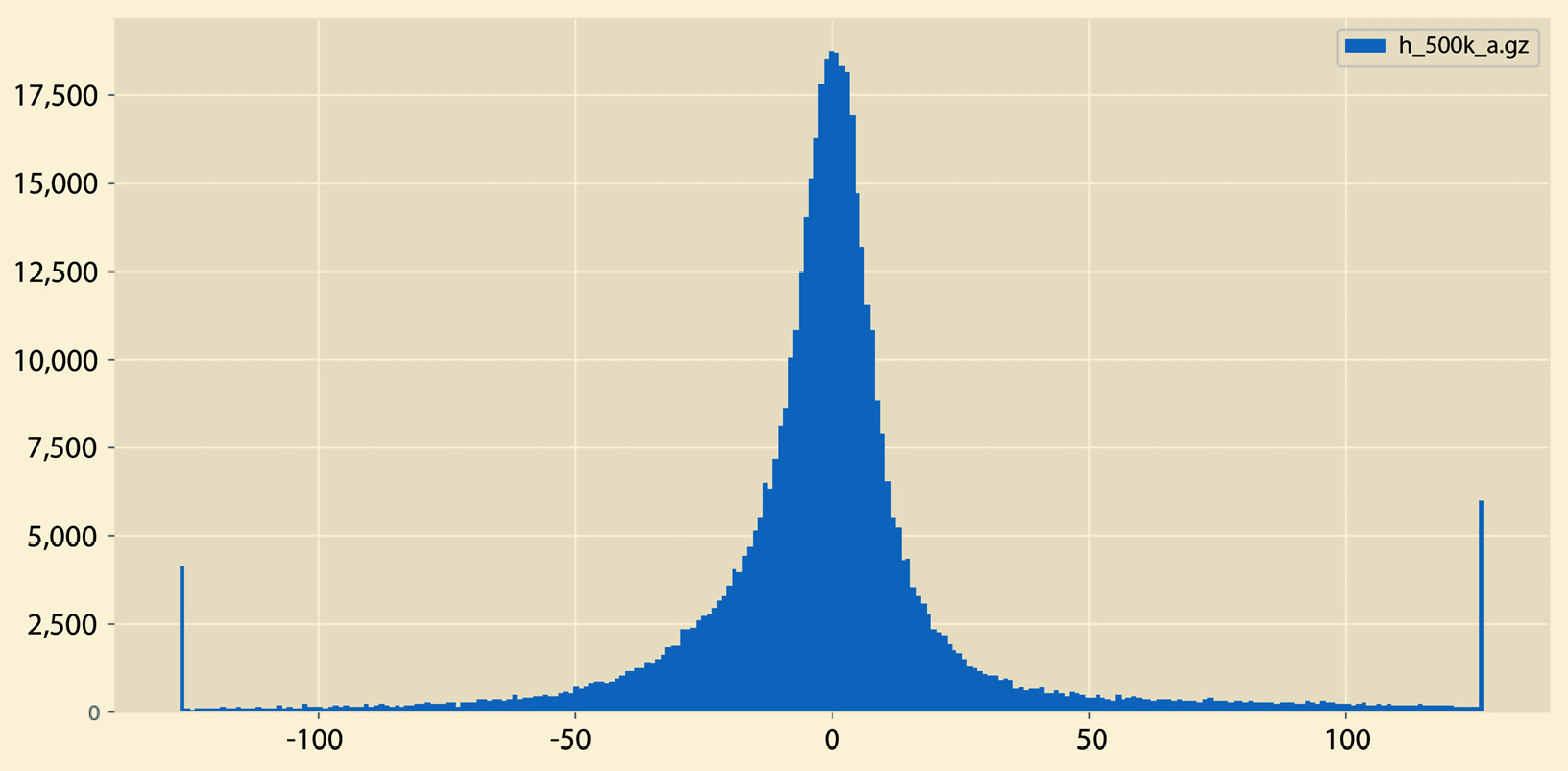
Figure 2.5 – A sample histogram

A different sample output from histogram.py can be seen in Figure 2.6:

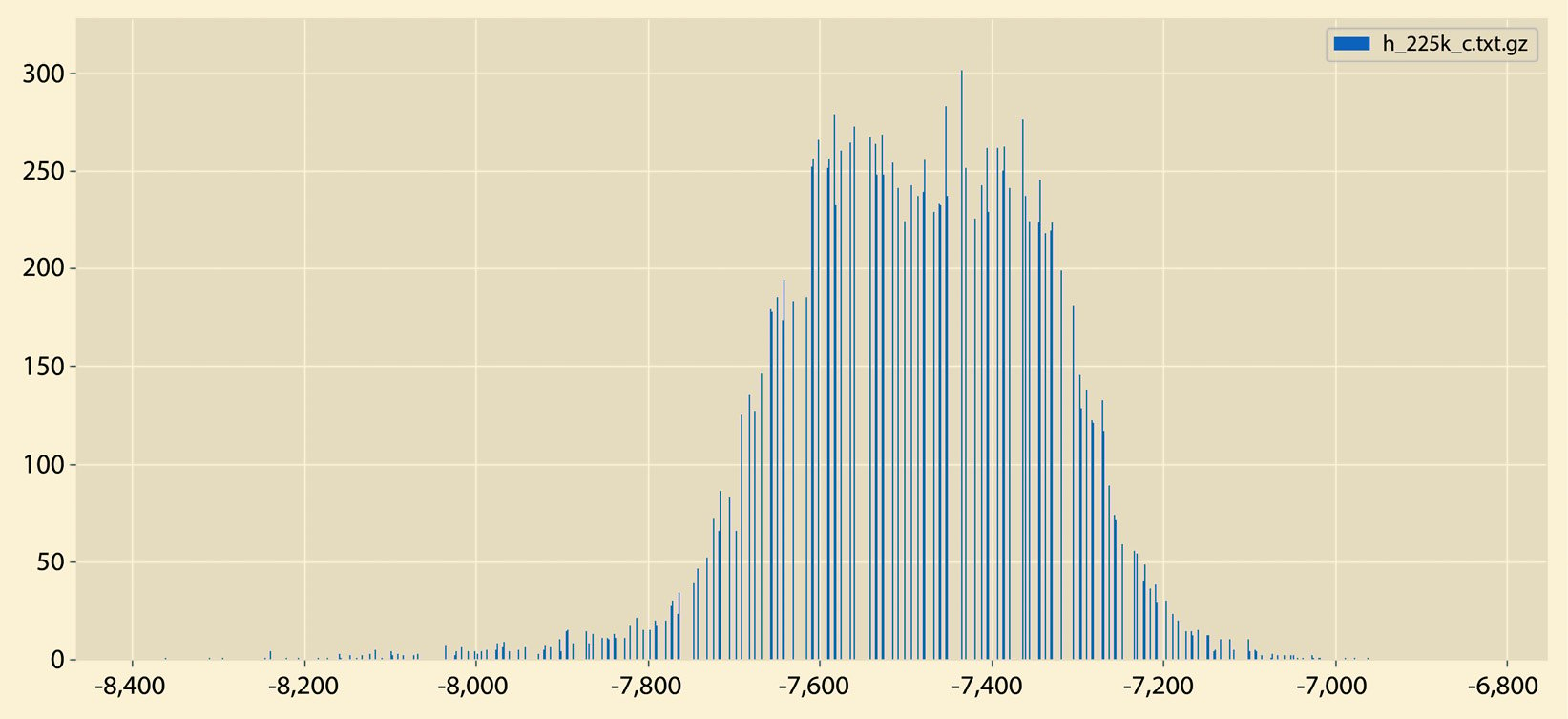
Figure 2.6 – A sample histogram

So, what is the difference between the histograms in Figure 2.5 and Figure 2.6? There exist many differences, including the fact that the histogram in Figure 2.5 does not have empty bins and it contains both negative and positive values. On the other hand, the histogram in Figure 2.6 contains negative values only that are far away from 0.

Now that we know about histograms, let us learn about another interesting statistical quantity – percentiles.

In this last bonus section of this chapter, we are going to learn how to compute the percentiles of a time series or a list (and if you find the information presented here difficult to understand, feel free to skip it). The main usage of such information is to better understand your time series data.

A percentile is a score where a given percentage of scores in the frequency distribution falls. Therefore, the 20th percentile is the score below which 20% of the scores of the distribution of the values of a dataset falls.

A quartile is one of the following three percentiles – 25%, 50%, or 75%. So, we have the first quartile, the second quartile, and the third quartile, respectively.

Both percentiles and quartiles are calculated in datasets sorted in ascending order. Even if you have not sorted that dataset, the relevant NumPy function, which is called quantile(), does that behind the scenes.

The Python code of percentiles.py is as follows:

#!/usr/bin/env python3
import sys
import pandas as pd
import numpy as np
def main():
     if len(sys.argv) != 2:
           print("TS")
           sys.exit()
     F = sys.argv[1]
     ts = pd.read_csv(F, compression='gzip')
     ta = ts.to_numpy()
     ta = ta.reshape(len(ta))
     per01 = round(np.quantile(ta, .01), 5)
     per25 = round(np.quantile(ta, .25), 5)
     per75 = round(np.quantile(ta, .75), 5)
     print("Percentile 1%:", per01, "Percentile 25%:", per25, "Percentile 75%:", per75)
if __name__ == '__main__':
     main()

All the work is done by the quantile() function of the NumPy package. Among other things, quantile() appropriately arranges its elements before performing any calculations. We do not know what happens internally, but most likely, quantile() sorts its input in ascending order.

The first parameter of quantile() is the NumPy array, and its second parameter is the percentage (percentile) that interests us. A 25% percentage is equal to the first quantile, a 50% percentage is equal to the second quantile, and a 75% percentage is equal to the third quantile. A 1% percentage is equal to the 1% percentile, and so on.

The output of percentiles.py is as follows:

$ ./percentiles.py ts1.gz
Percentile 1%: 1.57925 Percentile 25%: 7.15484 Percentile 75%: 23.2298

This chapter included the theory behind and practical implementation of SAX and an understanding of a time series from a statistical viewpoint. As the iSAX index construction is based on the SAX representation, we cannot construct an iSAX index without computing SAX representations.

Before you begin reading Chapter 3, please make sure that you know how to calculate the SAX representation of a time series or a subsequence, given the sliding window size, the number of segments, and the cardinality.

The next chapter contains the theory related to the iSAX index, shows you how to manually construct an iSAX index (which you will find very entertaining), and includes the development of some handy utilities.

• About Python packages: https://docs.python.org/3/reference/import.html
• The tsfresh package: https://pypi.org/project/tsfresh/
• The documentation for the tsfresh package can be found at https://tsfresh.readthedocs.io/en/latest/
• The scipy package: https://pypi.org/project/scipy/ and https://scipy.org/
• Normalization: https://en.wikipedia.org/wiki/Normalization_(statistics)
• Histogram: https://en.wikipedia.org/wiki/Histogram
• Percentile: https://en.wikipedia.org/wiki/Percentile
• Normal distribution: https://en.wikipedia.org/wiki/Normal_distribution

Try to solve the following exercises in Python:

• Divide by hand the y axis for the 16 = 24 cardinality. Did you divide it into 16 areas or 17 areas? How many breakpoints did you use?
• Divide by hand the y axis for the 64 = 26 cardinality. Did you divide it into 64 areas?
• Use the cardinality.py utility to plot the breakpoints of the 16 = 24 cardinality.
• Use the cardinality.py utility to plot the breakpoints of the 128 = 2 7 cardinality.
• Find the SAX representation of the {0, 2, -1, 2, 3, 4, -2, 4} subsequence using 4 segments and a cardinality of 4 (2 2). Do not forget to normalize it first.
• Find the SAX representation of the {0, 2, -1, 2, 3, 4, -2, 4} subsequence using 2 segments and a cardinality of 2 (2 1). Do not forget to normalize it first.
• Find the SAX representation of the {0, 2, -1, 2, 3, 1, -2, -4} subsequence using 4 segments and a cardinality of 2.
• Given the {0, -1, 1.5, -1.5, 0, 1, 0} time series and a sliding window size of 4, find the SAX representation of all its subsequences using 2 segments and a cardinality of 2.
• Create a synthetic time series and process it using using_tsfresh.py.
• Create a synthetic time series with 1,000 elements and process it using histogram.py.
• Create a synthetic time series with 5,000 elements and process it using histogram.py.
• Create a synthetic time series with 10,000 elements and process it using counting.py.
• Create a synthetic time series with 100 elements and process it using percentiles.py.
• Create a synthetic dataset with 100 elements and examine it using counting.py.
• Modify histogram.py to save its graphical output in a PNG file.
• Plot a time series using histogram.py and then process it using using_tsfresh.py