Electronic mail is a ubiquitous internet service for exchanging messages between people. A typical problem in this sphere of communication is identifying and blocking unsolicited and unwanted messages. Spam detectors undertake part of this role; ideally, they should not let spam escape uncaught while not obstructing any non-spam.

This chapter deals with this problem from a machine learning (ML) perspective and unfolds as a series of steps for developing and evaluating a typical spam detector. First, we elaborate on the limitations of performing spam detection using traditional programming. Next, we introduce the basic techniques for text representation and preprocessing. Finally, we implement two classifiers using an open source dataset and evaluate their performance based on standard metrics.

By the end of the chapter, you will be able to understand the nuts and bolts behind the different techniques and implement them in Python. But, more importantly, you should be capable of seamlessly applying the same pipeline to similar problems.

We go through the following topics:

• Obtaining the data
• Understanding its content
• Preparing the datasets for analysis
• Training classification models
• Realizing the tradeoffs of the algorithms
• Assessing the performance of the models

The code of this chapter is available as a Jupyter Notebook in the book’s GitHub repository: https://github.com/PacktPublishing/Machine-Learning-Techniques-for-Text/tree/main/chapter-02.

The Notebook has an in-built step to download the necessary Python modules required for the practical exercises in this chapter. Furthermore, for Windows, you need to download and install Microsoft C++ Build Tools from the following link: https://visualstudio.microsoft.com/visual-cpp-build-tools/.

A spam detector is software that runs on the mail server or our local computer and checks the inbox to detect possible spam. As with traditional letterboxes, an inbox is a destination for electronic mail messages. Generally, any spam detector has unhindered access to this repository and can perform tens, hundreds, or even thousands of checks per day to decide whether an incoming email is spam or not. Fortunately, spam detection is a ubiquitous technology that filters out irrelevant and possibly dangerous electronic correspondence.

How would you implement such a filter from scratch? Before exploring the steps together, look at a contrived (and somewhat naive) spam email message in Figure 2.1. Can you identify some key signs that differentiate this spam from a non-spam email?

Figure 2.1 – A spam email message

Even before reading the content of the message, most of you can immediately identify the scam from the email’s subject field and decide not to open it in the first place. But let’s consider a few signs (coded as T1 to T4) that can indicate a malicious sender:

• T1 – The text in the subject field is typical for spam. It is characterized by a manipulative style that creates unnecessary urgency and pressure.
• T2 – The message begins with the phrase Dear MR tjones. The last word was probably extracted automatically from the recipient’s email address.
• T3 – Bad spelling and the incorrect use of grammar are potential spam indicators.
• T4 – The text in the body of the message contains sequences with multiple punctuation marks or capital letters.

We can implement a spam detector based on these four signs, which we will hereafter call triggers. The detector classifies an incoming email as spam if T1, T2, T3, and T4 are True simultaneously. The following example shows the pseudocode for the program:

IF (subject is typical for spam)
    AND IF (message uses recipients email address)
        AND IF (spelling and grammar errors)
            AND IF (multiple sequences of marks-caps) THEN
                print("It's a SPAM!")

It’s a no-brainer that this is not the best spam filter ever built. We can predict that it blocks legitimate emails and lets some spam messages escape uncaught. We have to include more sophisticated triggers and heuristics to improve its performance in terms of both types of errors. Moreover, we need to be more specific about the cut-off thresholds for the triggers. For example, how many spelling errors (T3) and sequences (T4) make the relevant expressions in the pseudocode True? Is T3 an appropriate trigger in the first place? We shouldn’t penalize a sender for being bad at spelling! Also, what happens when a message includes many grammar mistakes but contains few sequences with capital letters? Can we still consider it spam? To answer these questions, we need data to support any claim. After examining a large corpus of messages annotated as spam or non-spam, we can safely extract the appropriate thresholds and adapt the pseudocode.

Can you think of another criterion? What about examining the message’s body and checking whether certain words appear more often? Intuitively, those words can serve as a way to separate the two types of emails. An easy way to perform this task is to visualize the body of the message using word clouds (also known as tag clouds). With this visualization technique, recurring words in the dataset (excluding articles, pronouns, and a few other cases) appear larger than infrequent ones.

One possible implementation of word clouds in Python is the word_cloud module (https://github.com/amueller/word_cloud). For example, the following code snippet presents how to load the email shown in Figure 2.1 from the spam.txt text file (https://github.com/PacktPublishing/Machine-Learning-Techniques-for-Text/tree/main/chapter-02/data), make all words lowercase, and extract the visualization:

# Import the necessary modules.
import matplotlib.pyplot as plt
from wordcloud import WordCloud
# Read the text from the file spam.txt.
text = open('./data/spam.txt').read()
# Create and configure the word cloud object.
wc = WordCloud(background_color="white", max_words=2000)
# Generate the word cloud image from the text.
wordcloud = wc.generate(text.lower())
# Display the generated image.
plt.imshow(wordcloud, interpolation='bilinear')
plt.axis("off")

Figure 2.2 shows the output plot:

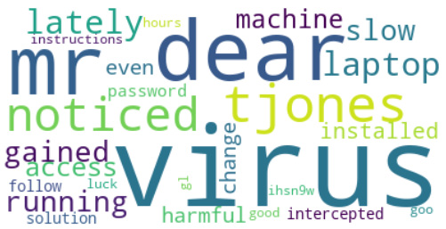
Figure 2.2 – A word cloud of the spam email

The image suggests that the most common word in our spam message is virus (all words are lowercase). Does the repetition of this word make us suspicious? Let’s suppose yes so that we can adapt the pseudocode accordingly:

     ...
            AND IF (multiple sequences of marks-caps) THEN
                AND IF (common word = "virus") THEN
                    print("It's a SPAM!")

Is this new version of the program better? Slightly. We can engineer even more criteria, but the problem becomes insurmountable at some point. It is not realistic to find all the possible suspicious conditions and deciphering the values of all thresholds by hand becomes an unattainable goal.

Notice that techniques such as word clouds are commonplace in ML problems to explore text data before resorting to any solution. We call this process Exploratory Data Analysis (EDA). EDA provides an understanding of where to direct our subsequent analysis and visualization methods are the primary tool for this task. We deal with this topic many times throughout the book.

It’s time to resort to ML to overcome the previous hurdles. The idea is to train a model from a corpus with labeled examples of emails and automatically classify new ones as spam or non-spam.

Explaining feature engineering

If you were being observant, you will have spotted that the input to the pseudocode was not the actual text of the message but the information extracted from it. For example, we used the frequency of the word virus, the number of sequences in capital letters, and so on. These are called features and the process of eliciting them is called feature engineering. For many years, this has been the central task of ML practitioners, along with calibrating (fine-tuning) the models.

Identifying a suitable list of features for any ML task requires domain knowledge – comprehending the problem you want to solve in-depth. Furthermore, how you choose them directly impacts the algorithm’s performance and determines its success to a significant degree. Feature engineering can be challenging, as we can overgenerate items in the list. For example, certain features can overlap with others, so including them in the subsequent analysis is redundant. On the other hand, specific features might be less relevant to the task because they do not accurately represent the underlying problem. Table 2.1 includes a few examples of good features:

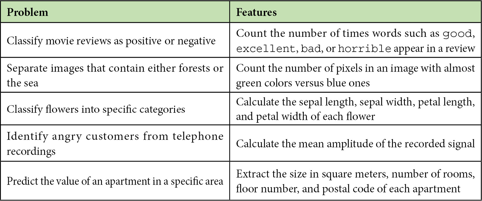
Table 2.1 – Examples of feature engineering

Given the preceding table, the rationale for devising features for any ML problem should be clear. First, we need to identify the critical elements of the problem under study and then decide how to represent each element with a range of values. For example, the value of an apartment is related to its size in square meters, which is a real positive number.

This section provided an overview of spam detection and why attacking this problem using traditional programming techniques is suboptimal. The reason is that identifying all the necessary execution steps manually is unrealistic. Then, we debated why extracting features from data and applying ML is more promising. In this case, we provide hints (as a list of features) to the program on where to focus, but it’s up to the algorithm to identify the most efficient execution steps.

The following section discusses how to extract the proper features in problems involving text such as emails, tweets, movie reviews, meeting transcriptions, or reports. The standard approach, in this case, is to use the actual words. Let’s see how.

What does a word mean to a computer? What about an image or an audio file? To put it simply, nothing. A computer circuit can only process signals that contain two voltage levels or states, similar to an on-off switch. This representation is the well-known binary system where every quantity is expressed as a sequence of 1s (high voltage) and 0s (low voltage). For example, the number 1001 in binary is 9 in decimal (the numerical system humans employ). Computers utilize this representation to encode the pixels of an image, the samples of an audio file, a word, and much more, as illustrated in Figure 2.3:

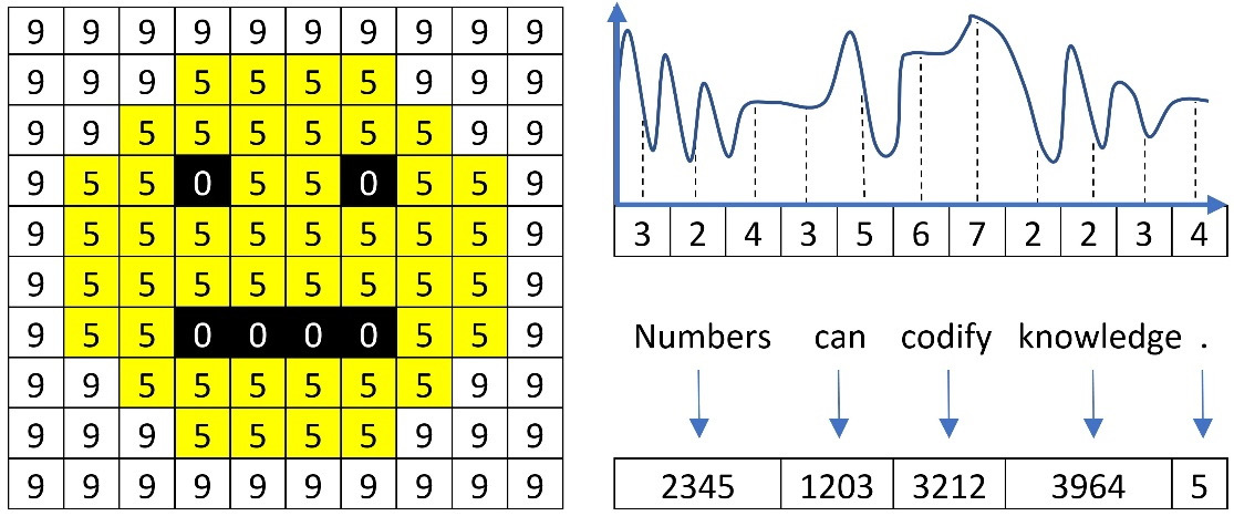
Figure 2.3 – Image pixels, audio samples, and words represented with numbers

Based on this representation, our computers can make sense of the data and process it the way we wish, such as by rendering an image on the screen, playing an audio track, or translating an input sentence into another language. As the book focuses on text, we will learn about the standard approaches for representing words in a piece of text data. More advanced techniques are a subject in the subsequent chapters.

Using label encoding

In ML problems, there are various ways to represent words; label encoding is the simplest form. For example, consider this quote from Aristotle: a friend to all is a friend to none. Using the label-encoding scheme and a dictionary with words to indices (a:0, all:1, friend:2, is:3, none:4, to:5), we can produce the mapping shown in Table 2.2:

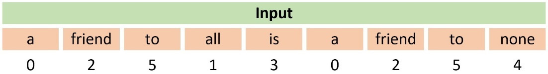
Table 2.2 – An example of using label encoding

We observe that a numerical sequence replaces the words in the sentence. For example, the word friend maps to the number 2. In Python, we can use the LabelEncoder class from the sklearn module and feed it with the quote from Aristotle:

from sklearn.preprocessing import LabelEncoder
# Create the label encoder and fit it with data.
labelencoder = LabelEncoder()
labelencoder.fit(["a", "all", "friend", "is", "none", "to"])
# Transform an input sentence.
x = labelencoder.transform(["a", "friend", "to", "all", "is", "a", "friend", "to", "none"])
print(x)
>> [0 2 5 1 3 0 2 5 4]

The output is the same array as the one in Table 2.2. There is a caveat, however. When an ML algorithm uses this representation, it implicitly considers and tries to exploit some kind of order among the words, for example, a<friend<to (because 0 < 2 < 5). This order does not exist in reality. On the other hand, label encoding is appropriate if there is an ordinal association between the words. For example, the good, better, and best triplet can be encoded as 1, 2, and 3, respectively. Another example is online surveys, where we frequently use categorical variables with predefined values for each question, such as disagree=-1, neutral=0, and agree=+1. In these cases, label encoding can be more appropriate, as the associations good<better<best and disagree<neutral<agree make sense.

Using one-hot encoding

Another well-known word representation technique is one-hot encoding, which codifies every word as a vector with zeros and a single one. Notice that the position of the one uniquely identifies a specific word; consequently, no two words exist with the same one-hot vector. Table 2.3 shows an example of this representation using the previous input sentence from Aristotle:

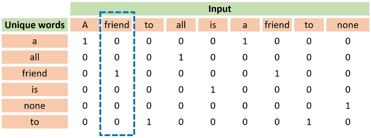
Table 2.3 – An example of using one-hot encoding

Observe that the first column in the table includes all unique words. The word friend appears at position 3, so its one-hot vector is [0, 0, 1, 0, 0, 0]. The more unique words in a dataset, the longer the vectors are because they depend on the vocabulary size.

In the code that follows, we use the OneHotEncoder class from the sklearn module:

from sklearn.preprocessing import OneHotEncoder
# The input.
X = [['a'], ['friend'], ['to'], ['all'], ['is'], ['a'], ['friend'], ['to'], ['none']]
# Create the one-hot encoder.
onehotencoder = OneHotEncoder()
# Fit and transform.
enc = onehotencoder.fit_transform(X).toarray()
print(enc.T)
>> [[1. 0. 0. 0. 0. 1. 0. 0. 0.]
 [0. 0. 0. 1. 0. 0. 0. 0. 0.]
 [0. 1. 0. 0. 0. 0. 1. 0. 0.]
 [0. 0. 0. 0. 1. 0. 0. 0. 0.]
 [0. 0. 0. 0. 0. 0. 0. 0. 1.]
 [0. 0. 1. 0. 0. 0. 0. 1. 0.]]

Looking at the code output, can you identify a drawback to this approach? The majority of the elements in the array are zeros. As the corpus size increases, so does the vocabulary size of the unique words. Consequently, we need bigger one-hot vectors where all other elements are zero except for one. Matrixes of this kind are called sparse and can pose challenges due to the memory required to store them.

Next, we examine another approach that addresses both ordinal association and sparsity issues.

Using token count encoding

Token count encoding, also known as the Bag-of-Words (BoW) representation, counts the absolute frequency of each word within a sentence or a document. The input is represented as a bag of words without taking into account grammar or word order. This method uses a Term Document Matrix (TDM) matrix that describes the frequency of each term in the text. For example, in Table 2.4, we calculate the number of times a word from a minimal vocabulary of seven words appears in Aristotle’s quote:

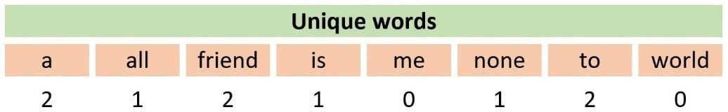
Table 2.4 – An example of using token count encoding

Notice that the corresponding cell in the table contains the value 0 when no such word is present in the quote. In Python, we can convert a collection of text documents to a matrix of token counts using the CountVectorizer class from the sklearn module, as shown in the following code:

from sklearn.feature_extraction.text import CountVectorizer
# The input.
X = ["a friend to all is a friend to none"]
# Create the count vectorizer.
vectorizer = CountVectorizer(token_pattern='[a-zA-Z]+')
# Fit and transform.
x = vectorizer.fit_transform(X)
print(vectorizer.vocabulary_)
>> {'a': 0, 'friend': 2, 'to': 5, 'all': 1, 'is': 3, 'none': 4}

Next, we print the token counts for the quote:

print(x.toarray()[0])
>> [2 1 2 1 1 2]

The CountVectorizer class takes the token pattern argument as the input [a-zA-Z]+, which identifies words with lowercase or uppercase letters. Don’t worry if the syntax of this pattern is not yet clear. We are going to demystify it later in the chapter. In this case, the code informs us that the word a (with id 0) appears twice, and therefore the first element in the output array [2, 1, 2, 1, 1, 2] is 2. Similarly, the word none, the fifth element of the array, appears once.

We can continue by extending the vectorizer using a property of human languages: the fact that certain word combinations are more frequent than others. We can verify this characteristic by performing Google searches of various word combinations inside double quotation marks. Each one yields a different number of search results, an indirect measure of their frequency in language.

When reading a spam email, we don’t usually focus on isolated words and instead identify patterns in word sequences that trigger an alert in our brain. How can we leverage this fact in our spam detection problem? One possible answer is to use n-grams as tokens for CountVectorizer. In simple terms, n-grams illustrate word sequences, and due to their simplicity and power, they have been extensively used in Natural Language Processing (NLP) applications. There are different variants of n-grams depending on the number of words that we group; for a single word, they are called unigrams; for two words, bigrams, and three words trigrams. Figure 2.4 presents the first three order n-grams for Aristotle’s quote:

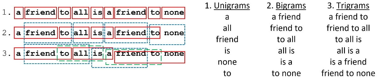
Figure 2.4 – Unigrams, bigrams, and trigrams for Aristotle’s quote

We used unigrams in the previous Python code, but we can now add the ngram_range argument during the vectorizer construction and use bigrams instead:

from sklearn.feature_extraction.text import CountVectorizer
# The input.
X = ["a friend to all is a friend to none"]
# Create the count vectorizer using bi-grams.
vectorizer = CountVectorizer(ngram_range=(2,2), token_pattern='[a-zA-Z]+')
# Fit and transform.
x = vectorizer.fit_transform(X)
print(vectorizer.vocabulary_)
>> {'a friend': 0, 'friend to': 2, 'to all': 4, 'all is': 1, 'is a': 3, 'to none': 5}

Next, we print the token counts for the quote:

print(x.toarray()[0])
>> [2 1 2 1 1 1]

In this case, the friend to bigram with an ID of 2 appears twice, so the third element in the output array is 2. For the same reason, the to none bigram (the last element) appears only once.

In this section, we discussed how to utilize word frequencies to encode a piece of text. Next, we will present a more sophisticated approach that uses word frequencies differently. Let’s see how.

Using tf-idf encoding

One limitation of BoW representations is that they do not consider the value of words inside the corpus. For example, if solely frequency were of prime importance, articles such as a or the would provide the most information for a document. Therefore, we need a representation that penalizes these frequent words. The remedy is the term frequency-inverse document frequency (tf-idf) encoding scheme that allows us to weigh each word in the text. You can consider tf-idf as a heuristic where more common words tend to be less relevant for most semantic classification tasks, and the weighting reflects this approach.

From a virtual dataset with 10 million emails, we randomly pick one containing 100 words. Suppose that the word virus appears three times in this email, so its term frequency (tf) is . Moreover, the same word appears in 1,000 emails in the corpus, so the inverse document frequency (idf) is equal to . The tf-idf weight is simply the product of these two statistics: . We reach a high tf-idf weight when we have a high frequency of the term in the random email and a low document frequency of the same term in the whole dataset. Generally, we calculate tf-idf weights with the following formula:

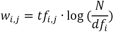
Where:

• Weight of word i in document j
• Frequency of word i in document j
• Total number of documents
• Number of documents containing word i

Performing the same calculations in Python is straightforward. In the following code, we use TfidfVectorizer from the sklearn module and a dummy corpus with four short sentences:

from sklearn.feature_extraction.text import TfidfVectorizer
# Create a dummy corpus.
corpus = [
        'We need to meet tomorrow at the cafeteria.',
        'Meet me tomorrow at the cafeteria.',
        'You have inherited millions of dollars.',
        'Millions of dollars just for you.']
# Create the tf-idf vectorizer.
vectorizer = TfidfVectorizer()
# Generate the tf-idf matrix.
tfidf = vectorizer.fit_transform(corpus)

Next, we print the result as an array:

print(tfidf.toarray())
>> [[0.319  0.319    0.       0.      0.       0.
  0.        0.       0.319    0.      0.404    0.
  0.319     0.404    0.319    0.404   0.]
 [0.388     0.388    0.       0.      0.       0.
  0.        0.493    0.388    0.      0.       0.
  0.388     0.       0.388    0.      0.]
 [0.        0.       0.372    0.      0.472    0.472
  0.        0.       0.       0.372   0.       0.372
  0.        0.       0.       0.      0.372]
 [0.        0.       0.372    0.472   0.       0.
  0.472     0.       0.       0.372   0.    0.372
  0.        0.       0.       0.      0.372]]

What does this output tell us? Each of the four sentences is encoded with one tf-idf vector of 17 elements (this is the number of unique words in the corpus). Non-zero values show the tf-idf weight for a word in the sentence, whereas a value equal to zero signifies the absence of the specific word. If we could somehow compare the tf-idf vectors of the examples, we can tell which pair resembles more. Undoubtedly, 'You have inherited millions of dollars.' is closer to 'Millions of dollars just for you.' than the other two sentences. Can you perhaps guess where this discussion is heading? By calculating an array of weights for all the words in an email, we can compare it with the reference arrays of spam or non-spam and classify it accordingly. The following section will tell us how.

Calculating vector similarity

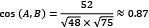
Mathematically, there are different ways to calculate vector resemblances, such as cosine similarity (cs) or Euclidean distance. Specifically, cs is the degree to which two vectors point in the same direction, targeting orientation rather than magnitude (see Figure 2.5).

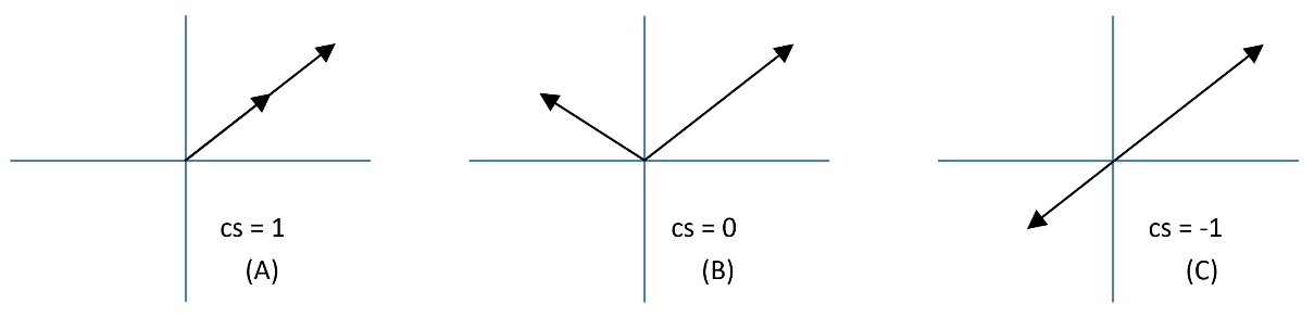
Figure 2.5 – Three cases of cosine similarity

When the two vectors point in the same direction, the cs equals 1 (in A in Figure 2.5); when they are perpendicular, it is 0 (in B in Figure 2.5), and when they point in opposite directions, it is -1 (in C in Figure 2.5). Notice that only values between 0 to 1 are valid in NLP applications since the term frequencies cannot be negative.

Consider now an example where A, B, and C are vectors with three elements each, so that A = (4, 4, 4), B = (1, 7, 5), and C = (-5, 5, 1). You can think of each number in the vector as a coordinate in an xyz-space. Looking at Figure 2.6, A and B seem more similar than C. Do you agree?

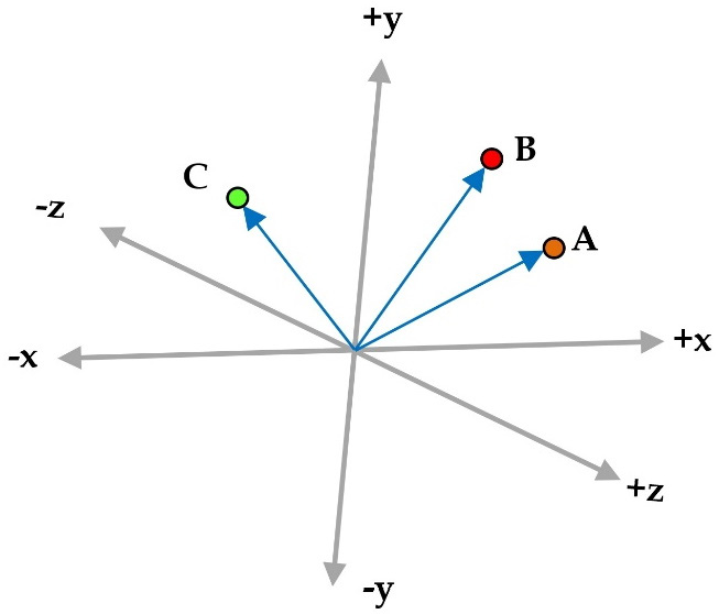
Figure 2.6 – Three vectors A, B, and C in a three-dimensional space

We calculate the dot product (signified with the symbol •) between two vectors of the same size by multiplying their elements in the same position. and are two vectors, so their dot product is . In our example, and . Additionally, the magnitude of the vector is defined as 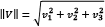and in our case, 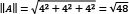, , and .

Therefore, we obtain the following:

, , and .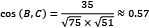

The results confirm our first hypothesis that A and B are more similar than C.

In the following code, we calculate the cs of the tf-idf vectors between the corpus’s first and second examples:

from sklearn.metrics.pairwise import cosine_similarity
# Convert the matrix to an array.
tfidf_array = tfidf.toarray()
# Calculate the cosine similarity between the first amd second example.
print(cosine_similarity([tfidf_array[0]], [tfidf_array[1]]))
>> [[0.62046087]]

We also repeat the same calculation between all tf-idf vectors:

# Calculate the cosine similarity among all examples.
print(cosine_similarity(tfidf_array))
>> [[1.         0.62046     0.        0.        ]
 [0.62046       1.          0.        0.        ]
 [0.            0.          1.        0.5542    ]
 [0.            0.          0.5542    1.        ]]

As expected, the value between the first and second examples is high and equal to 0.62. Between the first and the third example, it is 0, 0.55 between the third and the fourth, and so on.

Exploring tf-idf has concluded our discussion on the standard approaches for representing text data. The importance of this step should be evident, as it relates to the machine’s ability to create models that better understand textual input. Failing to get good representations of the underlying data typically leads to suboptimal results in the later phases of analysis. We will also encounter a powerful representation technique for text data in Chapter 3, Classifying Topics of Newsgroup Posts.

In the next section, we will go a step further and discuss different techniques of preprocessing data that can boost the performance of ML algorithms.

During the tf-idf discussion, we mentioned that articles often do not help convey the critical information in a document. What about words such as but, for, or by? Indeed, they are ubiquitous in English texts but probably not very useful for our task. This section focuses on four techniques that help us remove noise from the data and reduce the problem’s complexity. These techniques constitute an integral part of the data preprocessing phase, which is crucial before applying more sophisticated methods to the text data. The first technique involves splitting an input text into meaningful chunks, while the second teaches us how to remove low informational value words from the text—the last two focus on mapping each word to a root form.

Tokenizing the input

So far, we have used the term token with the implicit assumption that it always refers to a word (or an n-gram) independently of the underlying NLP task. Tokenization is a more general process where we split textual data into smaller components called tokens. These can be words, phrases, symbols, or other meaningful elements. We perform this task using the nltk toolkit and the word_tokenize method in the following code:

# Import the toolkit.
import nltk
nltk.download('punkt')
# Tokenize the input text.
wordTokens = nltk.word_tokenize("a friend to all is a friend to none")
print(wordTokens)
>> ['a', 'friend', 'to', 'all', 'is', 'a', 'friend', 'to', 'none']

As words are the tokens of a sentence, sentences are the tokens of a paragraph. For the latter, we can use another method in nltk called sent_tokenize and tokenize a paragraph with three sentences:

# Tokenize the input paragraph.
sentenceTokens = nltk.sent_tokenize("A friend to all is a friend to none. A friend to none is a friend to all. A friend is a friend.")
print(sentenceTokens)
>> ['A friend to all is a friend to none.', 'A friend to none is a friend to all.', 'A friend is a friend.']

This method uses the full stop as a delimiter (as in, a character to separate the text strings) and the output in our example is a list with three elements. Notice that using the full stop as a delimiter is not always the best solution. For example, the text can contain abbreviations; thus, more sophisticated solutions are required to compensate for this situation.

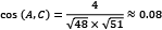
In the Using token count encoding section, we saw how CountVectorizer used a pattern to split the input into multiple tokens and promised to demystify its syntax later in the chapter. So, it’s time to introduce regular expressions (regexp) that can assist with the creation of a tokenizer. These expressions are used to find a string in a document, replace part of the text with something else, or examine the conformity of some textual input. We can improvise very sophisticated matching patterns and mastering this skill demands time and effort. Recall that the unstructured nature of text data means that it requires preprocessing before it can be used for analysis, so regexp are a powerful tool for this task. The following table shows a few typical examples:

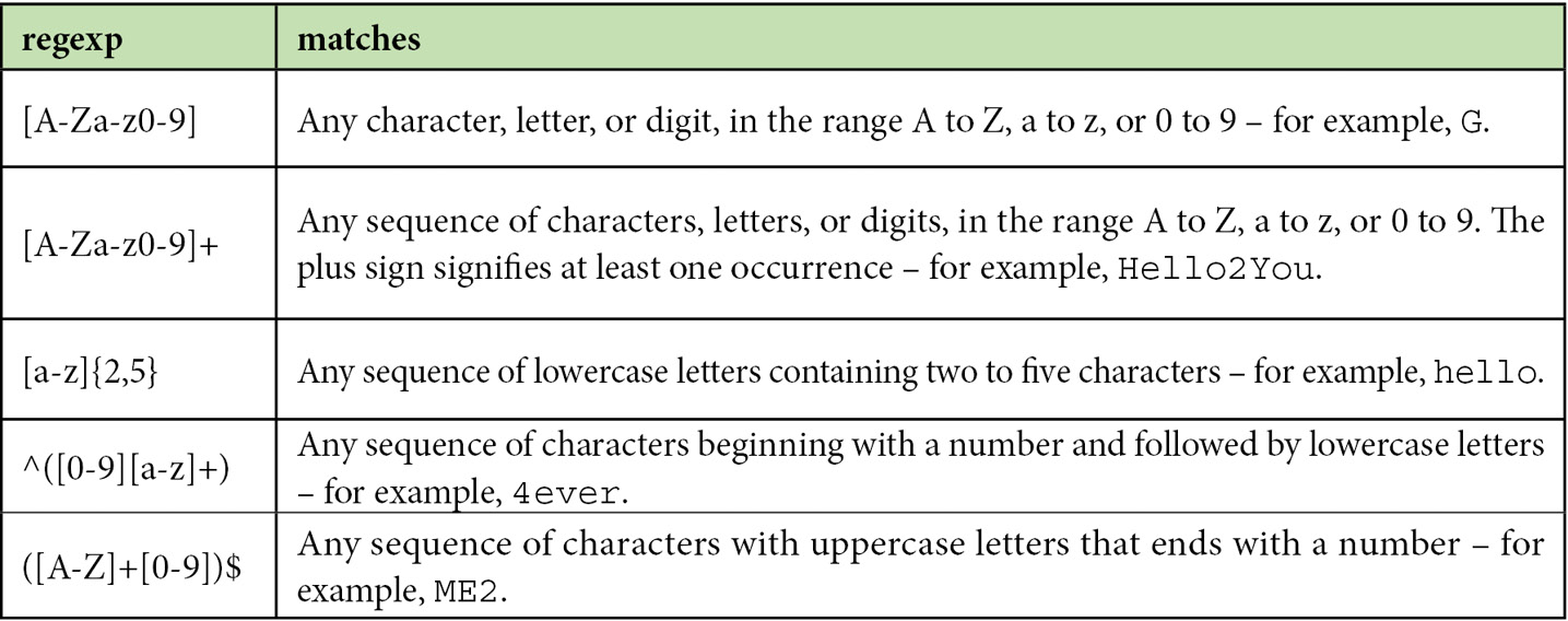
Table 2.5 – Various examples of regular expressions

A pattern using square brackets ([]) matches character ranges. For example, the [A-Z] regexp matches Q because it is part of the range of capital letters from A to Z. Conversely, the same lowercase character is not matched. Quantifiers inside curly braces match repetitions of patterns. In this case, the [A-Z]{3} regexp matches a sequence of BCD. The ^ and $ characters match a pattern at the beginning and end of a sentence, respectively. For example, the ^[0-9] regexp matches a 4ever string, as it starts with the number four. The + symbol matches one or more repetitions of the pattern, while * matches zero or more repetitions. A dot, ., is a wildcard for any character.

We can go a step further and analyze a more challenging regexp. Most of us have already used web forms that request an email address input. When the provided email is not valid, an error message is displayed. How does the web form recognize this problem? Obviously, by using a regexp! The general format of an email address contains a local-part, followed by an @ symbol, and then by a domain – for example, local-part@domain. Figure 2.7 analyzes a regexp that can match this format:

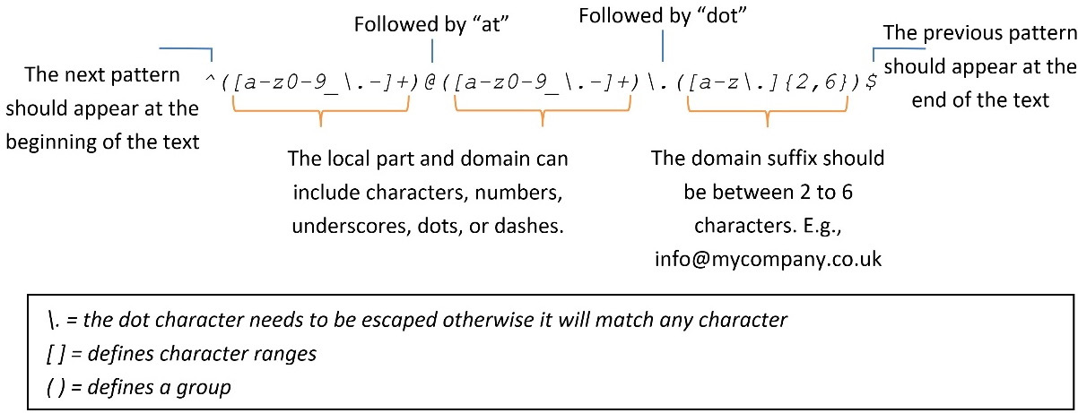
Figure 2.7 – A regexp for checking the validity of an email address

This expression might seem overwhelming and challenging to understand, but things become apparent if you examine each part separately. Escaping the dot character is necessary to remove its special meaning in the context of a regexp and ensure that it is used literally. Specifically, ., a regexp, matches any word, whereas \. matches only a full stop.

To set things into action, we tokenize a valid and an invalid email address using the regexp from Figure 2.7:

# Create the Regexp tokenizer.
tokenizer = nltk.tokenize.RegexpTokenizer(pattern='^([a-z0-9_\.-]+)@([a-z0-9_\.-]+)\.([a-z\.]{2,6})$')
# Tokenize a valid email address.
tokens = tokenizer.tokenize("john@doe.com")
print(tokens)
>> [('john', 'doe', 'com')]

The output tokens for the invalid email are as follows:

# Tokenize a non-valid email address.
tokens = tokenizer.tokenize("john-AT-doe.com")
print(tokens)
>> []

In the first case, the input, john@doe.com, is parsed as expected, as the address’s local-part, domain, and suffix are provided. Conversely, the second input does not comply with the pattern (it misses the @ symbol), and consequently, nothing is printed in the output.

There are many other situations where we need to craft particular regexps for identifying patterns in a document, such as HTML tags, URLs, telephone numbers, and punctuation marks. However, that’s the scope of another book!

Removing stop words

A typical task during the preprocessing phase is removing all the words that presumably help us focus on the most important information in the text. These are called stop words and there is no universal list in English or any other language. Examples of stop words include determiners (such as another and the), conjunctions (such as but and or), and prepositions (such as before and in). Many online sources are available that provide lists of stop words and it’s not uncommon to adapt their content according to the problem under study. In the following example, we remove all the stop words from a spam text using a built-in set from a wordcloud module named STOPWORDS. We also include three more words in the set to demonstrate its functionality:

from wordcloud import WordCloud, STOPWORDS
# Read the text from the file data.txt.
text = open('./data/spam.txt').read()
# Get all stopwords and update with few others.
sw = set(STOPWORDS)
sw.update(["dear", "virus", "mr"])
# Create and configure the word cloud object.
wc = WordCloud(background_color="white", stopwords=sw, max_words=2000)

Next, we generate the word cloud plot:

# Generate the word cloud image from the text.
wordcloud = wc.generate(text.lower())
# Display the generated image.
plt.imshow(wordcloud, interpolation='bilinear')
plt.axis("off")

The output is illustrated in Figure 2.8:

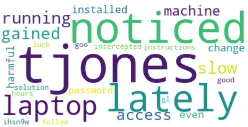
Figure 2.8 – A word cloud of the spam email after removing the stop words

Take a moment to compare it with the one in Figure 2.2. For example, the word virus is missing in the new version, as this word was part of the list of stop words.

The following section will cover another typical step of the preprocessing phase.

Stemming the words

Removing stop words is, in essence, a way to extract the juice out of the corpus. But we can squeeze the lemon even more! Undoubtedly, every different word form encapsulates a special meaning that adds richness and linguistic diversity to a language. These variances, however, result in data redundancy that can lead to ineffective ML models. In many practical applications, we can map words with the same core meaning to a central word or symbol and thus reduce the input dimension for the model. This reduction can be beneficial to the performance of the ML or NLP application.

This section introduces a technique called stemming that maps a word to its root form. Stemming is the process of cutting off the end (suffix) or the beginning (prefix) of an inflected word and ending up with its stem (the root word). So, for example, the stem of the word plays is play. The most common algorithm in English for performing stemming is the Porter stemmer, which consists of five sets of rules (https://tartarus.org/martin/PorterStemmer/) applied sequentially to the word. For example, one rule is to remove the “-ed” suffix from a word to obtain its stem only if the remainder contains at least one vowel. Based on this rule, the stem of played is play, but the stem for led is still led.

Using the PorterStemmer class from nltk in the following example, we observe that all three forms of play have the same stem:

# Import the Porter stemmer.
from nltk.stem import PorterStemmer
# Create the stemmer.
stemmer = PorterStemmer()
# Stem the words 'playing', 'plays', 'played'.
stemmer.stem('playing')
>> 'play'

Let’s take the next word:

stemmer.stem('plays')
>> 'play'

Now, check played:

stemmer.stem('played')
>> 'play'

Notice that the output of stemming doesn’t need to be a valid word:

# Stem the word 'bravery'
stemmer.stem('bravery')
>> 'braveri'

We can even create our stemmer using regexps and the RegexpStemmer class from nltk. In the following example, we search for words with the ed suffix:

# Import the Porter stemmer
from nltk.stem import RegexpStemmer
# Create the stemmer matching words ending with 'ed'.
stemmer = RegexpStemmer('ed')
# Stem the verbs 'playing', 'plays', 'played'.
stemmer.stem('playing')
>> 'playing'

Let’s check the next word:

stemmer.stem('plays')
>> 'plays'

Now, take another word:

stemmer.stem('played')
>> 'play'

The regexp in the preceding code matches played; therefore, the stemmer outputs play. The two other words remain unmatched, and for that reason, no stemming is applied. The following section introduces a more powerful technique to achieve similar functionality.

Lemmatizing the words

Lemmatization is another sophisticated approach for reducing the inflectional forms of a word to a base root. The method performs morphological analysis of the word and obtains its proper lemma (the base form under which it appears in a dictionary). For example, the lemma of goes is go. Lemmatization differs from stemming, as it requires detailed dictionaries to look up a word. For this reason, it’s slower but more accurate than stemming and more complex to implement.

WordNet (https://wordnet.princeton.edu/) is a lexical database for the English language created by Princeton University and is part of the nltk corpus. Superficially, it resembles a thesaurus in that it groups words based on their meanings. WordNet is one way to use lemmatization inside nltk. In the example that follows, we extract the lemmas of three English words:

# Import the WordNet Lemmatizer.
from nltk.stem import WordNetLemmatizer
nltk.download('wordnet')
nltk.download('omw-1.4')
# Create the lemmatizer.
lemmatizer = WordNetLemmatizer()
# Lemmatize the verb 'played'.
lemmatizer.lemmatize('played', pos='v')
>> 'play'

Observe that the lemma for played is the same as its stem, play. On the other hand, the lemma and stem differ for led (lead versus led, respectively):

# Lemmatize the verb 'led'.
lemmatizer.lemmatize('led', pos='v')
>> 'lead'

There are also situations where the same lemma corresponds to words with different stems. The following code shows an example of this case where good and better have the same lemma but not the same stem:

# Lemmatize the adjective 'better'.
lemmatizer.lemmatize('better', pos='a')
>> 'good'

The differences between lemmatization and stemming should be apparent from the previous examples. Remember that we use either method on a given dataset and not both simultaneously.

The focus of this section has been on four typical techniques for preprocessing text data. In the case of word representations, the way we apply this step impacts the model’s performance. In many similar situations, identifying which technique works better is a matter of experimentation. The following section presents how to implement classifiers using an open source corpus for spam detection.

Up until this point, we have learned how to represent and preprocess text data. It’s time to make use of this knowledge and create the spam classifier. First, we put all the pieces together using a publicly available corpus. Before we proceed to the training of the classifier, we need to follow a series of typical steps that include the following:

1. Getting the data
2. Splitting it into a training and test set
3. Preprocessing its content
4. Extracting the features

Let’s examine each step one by one.

Getting the data

The SpamAssassin public mail corpus (https://spamassassin.apache.org/old/publiccorpus/) is a selection of email messages suitable for developing spam filtering systems. It offers two variants for the messages, either in plain text or HTML formatting. For simplicity, we will use only the first type in this exercise. Parsing HTML text requires special handling – for example, implementing your own regexps! The term coined to describe the opposite of spam emails is ham since the two words are related to meat products (spam refers to canned ham). The dataset contains various examples divided into different folders according to their complexity. This exercise uses the files within these two folders: spam_2 (https://github.com/PacktPublishing/Machine-Learning-Techniques-for-Text/tree/main/chapter-02/data/20050311_spam_2/spam_2) for spam and hard_ham (https://github.com/PacktPublishing/Machine-Learning-Techniques-for-Text/tree/main/chapter-02/data/20030228_hard_ham/hard_ham) for ham.

Creating the train and test sets

Initially, we read the messages for the two categories (ham and spam) and split them into training and testing groups. As a rule of thumb, we can choose a 75:25 (https://en.wikipedia.org/wiki/Pareto_principle) split between the two sets, attributing a more significant proportion to the training data. Note that other ratios might be preferable depending on the size of the dataset. Especially for massive corpora (with millions of labeled instances), we can create test sets with just 1% of the data, which is still a significant number. To clarify this process, we divide the code into the following steps:

1. First, we load the ham and spam datasets using the train_test_split method. This method controls the size of the training and test sets for each case and the samples that they include:

   import email
   import glob
   import numpy as np
   from operator import is_not
   from functools import partial
   from sklearn.model_selection import train_test_split
   # Load the path for each email file for both categories.
   ham_files = train_test_split(glob.glob('./data/20030228_hard_ham/hard_ham/*'), random_state=123)
   spam_files = train_test_split(glob.glob('./data/20050311_spam_2/spam_2/*'), random_state=123)

2. Next, we read the content of each email and keep the ones without HTML formatting:

   # Method for getting the content of an email.
   def get_content(filepath):
       file = open(filepath, encoding='latin1')
       message = email.message_from_file(file)
       for msg_part in message.walk():
           # Keep only messages with text/plain content.
           if msg_part.get_content_type() == 'text/plain':
               return msg_part.get_payload()
   # Get the training and testing data.
   ham_train_data = [get_content(i) for i in ham_files[0]]
   ham_test_data = [get_content(i) for i in ham_files[1]]
   spam_train_data = [get_content(i) for i in spam_files[0]]
   spam_test_data = [get_content(i) for i in spam_files[1]]

3. For our analysis, we exclude emails with empty content. The filter method with None as the first argument removes any element that includes an empty string. Then, the filtered output is used to construct a new list using list:

   # Keep emails with non-empty content.
   ham_train_data = list(filter(None, ham_train_data))
   ham_test_data = list(filter(None, ham_test_data))
   spam_train_data = list(filter(None, spam_train_data))
   spam_test_data = list(filter(None, spam_test_data))

4. Now, let’s merge the spam and ham training sets into one (do the same for their test sets):

   # Merge the train/test files for both categories.
   train_data = np.concatenate((ham_train_data, spam_train_data))
   test_data = np.concatenate((ham_test_data, spam_test_data))

5. Finally, we assign a class label for each of the two categories (ham and spam) and merge them into common training and test sets:

   # Assign a class for each email (ham = 0, spam = 1).
   ham_train_class = [0]*len(ham_train_data)
   ham_test_class = [0]*len(ham_test_data)
   spam_train_class = [1]*len(spam_train_data)
   spam_test_class = [1]*len(spam_test_data)
   # Merge the train/test classes for both categories.
   train_class = np.concatenate((ham_train_class, spam_train_class))
   test_class = np.concatenate((ham_test_class, spam_test_class))

Notice that in step 1, we also pass random_state in the train_test_split method to make all subsequent results reproducible. Otherwise, the method performs a different data shuffling in each run and produces random splits for the sets.

In this section, we have learned how to read text data from a set of files and keep the information that makes sense for the problem under study. After this point, the datasets are suitable for the next processing phase.

Preprocessing the data

It’s about time to use the typical data preprocessing techniques that we learned earlier. These include tokenization, stop word removal, and lemmatization. Let’s examine the steps one by one:

1. First, let’s tokenize the train or test data:

   from nltk.stem import WordNetLemmatizer
   from nltk.tokenize import word_tokenize
   from sklearn.feature_extraction.text import ENGLISH_STOP_WORDS
   # Tokenize the train/test data.
   train_data = [word_tokenize(i) for i in train_data]
   test_data = [word_tokenize(i) for i in test_data]

2. Next, we remove the stop words by iterating over the input examples:

   # Method for removing the stop words.
   def remove_stop_words(input):
       result = [i for i in input if i not in ENGLISH_STOP_WORDS]
       return result
   # Remove the stop words.
   train_data = [remove_stop_words(i) for i in train_data]
   test_data = [remove_stop_words(i) for i in test_data]

3. Now, we create the lemmatizer and apply it to the words:

   # Create the lemmatizer.
   lemmatizer = WordNetLemmatizer()
   # Method for lemmatizing the text.
   def lemmatize_text(input):
       return [lemmatizer.lemmatize(i) for i in input]
   # Lemmatize the text.
   train_data = [lemmatize_text(i) for i in train_data]
   test_data = [lemmatize_text(i) for i in test_data]

4. Finally, we reconstruct the data in the two sets by joining the words separated by a space and return the concatenated string:

   # Reconstruct the data.
   train_data = [" ".join(i) for i in train_data]
   test_data = [" ".join(i) for i in test_data]

As a result, we have at our disposal two Python lists, namely train_data and test_data, containing the initial text data in a processed form suitable for proceeding to the next phase.

Extracting the features

We continue with the extraction of the features of each sentence in the previously created datasets. This step uses tf-idf vectorization after training the vectorizer with the training data. There is a problem though, as the vocabulary in the training and test sets might differ. In this case, the vectorizer ignores unknown words, and depending on the mismatch level, we might get suboptimal representations for the test set. Hopefully, as more data is added to any corpus, the mismatch becomes smaller, so ignoring a few words has a negligible practical impact. An obvious question is – why not train the vectorizer with the whole corpus before the split? However, this engenders the risk of getting performance measures that are too optimistic later in the pipeline, as the model has seen the test data at some point. As a rule of thumb, always keep the test set separate and only use it to evaluate the model.

In the code that follows, we vectorize the data in both the training and test sets using tf-idf:

from sklearn.feature_extraction.text import TfidfVectorizer
# Create the vectorizer.
vectorizer = TfidfVectorizer()
# Fit with the train data.
vectorizer.fit(train_data)
# Transform the test/train data into features.
train_data_features = vectorizer.transform(train_data)
test_data_features = vectorizer.transform(test_data)

Now, the training and test sets are transformed from sequences of words to numerical vectors. From this point on, we can apply any sophisticated algorithm we wish, and guess what? This is what we are going to do in the following section!

Introducing the Support Vector Machines algorithm

It’s about time that we train the first classification model. One of the most well-known supervised learning algorithms is the Support Vector Machines (SVM) algorithm. We could dedicate a whole book to demystifying this family of methods, so we will visit a few key elements in this section. First, recall from Chapter 1, Introducing Machine Learning for Text, that any ML algorithm creates decision boundaries to classify new data correctly. As we cannot sketch high-dimensional spaces, we will consider a two-dimensional example. Hopefully, this provides some of the intuition behind the algorithm.

Figure 2.9 shows the data points for the spam and ham instances along with two features, namely and :

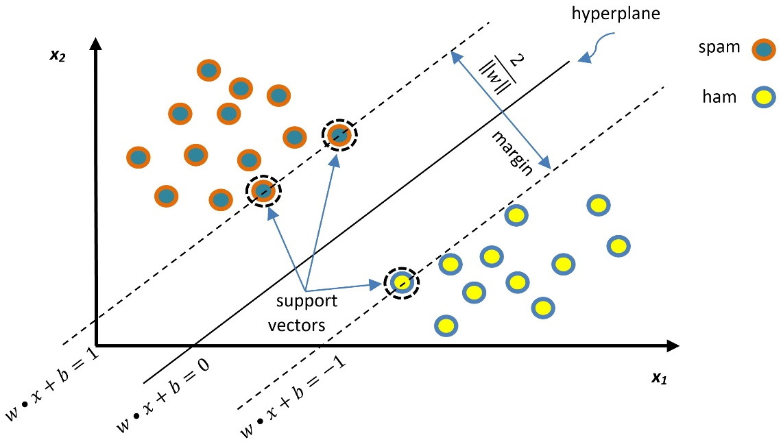
Figure 2.9 – Classification of spam and ham emails using the SVM

The line in the middle separates the two classes and the dotted lines represent the borders of the margin. The SVM has a twofold aim to find the optimal separation line (a one-dimensional hyperplane) while maximizing the margin. Generally, for an n-dimensional space, the hyperplane has (n-1) dimensions. Let’s examine our space size in the code that follows:

print(train_data_features.shape)
>> (670, 28337)

Each of the 670 emails in the training set is represented by a feature vector with a size of 28337 (the number of unique words in the corpus). In this sparse vector, the non-zero values signify the tf-idf weights for the words. For the SVM, the feature vector is a point in a 28,337-dimensional space, and the problem is to find a 28,336-dimensional hyperplane to separate those points. One crucial consideration within the SVM is that not all the data points contribute equally to finding the optimal hyperplane, but mostly those close to the margin boundaries (depicted with a dotted circle in Figure 2.9). These are called support vectors, and if they are removed, the position of the dividing hyperplane alters. For this reason, we consider them the critical part of the dataset.

The general equation of a line in two-dimensional space is expressed with the formula . Three examples are shown in Figure 2.10:

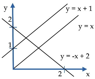
Figure 2.10 – Examples of line equations

In the same sense, the middle line in Figure 2.9 and the two margin boundaries have the following equations, respectively:

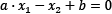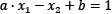, and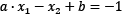

Defining the vectors and , we can rewrite the previous equations using the dot product that we encountered in the Calculating vector similarity section:

, , and

To find the best hyperplane, we need to estimate w and b, referred to as the weight and bias in ML terminology. Among the infinite number of lines that separate the two classes, we need to find the one that maximizes the margin, the distance between the closest data points of the two classes. In general, the distance between two parallel lines 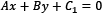and 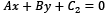is equal to the following:

So, the distance between the two margin boundaries is the following:

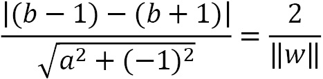
To maximize the previous equation, we need to minimize the denominator, namely the quantity that represents the Euclidean norm of vector w. The technique for finding w and b is beyond the scope of this book, but we need to define and solve a function that penalizes any misclassified examples within the margin. After this point, we can classify a new example, , based on the following model (the sign function takes any number as input and returns +1 if it is positive or -1 if it is negative):

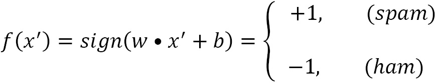
The example we are considering in Figure 2.9 represents an ideal situation. The data points are arranged in the two-dimensional space in such a way that makes them linearly separable. However, this is often not the case, and the SVM incorporates kernel functions to cope with nonlinear classification. Describing the mechanics of these functions further is beyond the scope of the current book. Notice that different kernel functions are available, and as in all ML problems, we have to experiment to find the most efficient option in any case. But before using the algorithm, we have to consider two important issues to understand the SVM algorithm better.

Adjusting the hyperparameters

Suppose two decision boundaries (straight lines) can separate the data in Figure 2.11.

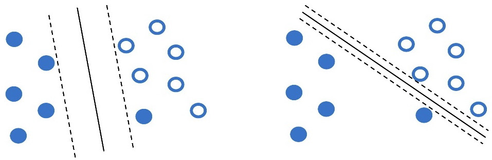
Figure 2.11 – Two possible decision boundaries for the data points using the SVM

Which one of those boundaries do you think works better? The answer, as in most similar questions, is that it depends! For example, the line in the left plot has a higher classification error, as one opaque dot resides on the wrong side. On the other hand, the margin in the right plot (distance between the dotted lines) is small, and therefore the model lacks generalization. In most cases, we can tolerate a small number of misclassifications during SVM training in favor of a hyperplane with a significant margin. This technique is called soft margin classification and allows some samples to be on the wrong side of the margin.

The SVM algorithm permits the adjustment of the training accuracy versus generalization tradeoff using the hyperparameter C. A frequent point of confusion is that hyperparameters and model parameters are the same things, but this is not true. Hyperparameters are parameters whose values are used to control the learning process. On the other hand, model parameters update their value in every training iteration until we obtain a good classification model. We can direct the SVM to create the most efficient model for each problem by adjusting the hyperparameter C. The left plot of Figure 2.11 is related to a lower C value compared to the one on the right.

Let’s look at another dataset for which two possible decision boundaries exist (Figure 2.12). Which one seems to work better this time?

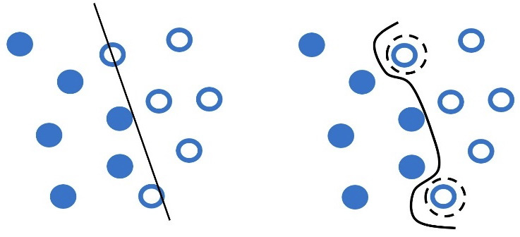
Figure 2.12 – Generalization (left) versus overfitting (right)

At first glance, the curved line in the plot on the right perfectly separates the data into two classes. But there is a problem. Getting too specific boundaries entails the risk of overfitting, where your model learns the training data perfectly but fails to classify a slightly different example correctly.

Consider the following real-world analogy of overfitting. Most of us have grown in a certain cultural context, trained (overfitted) to interpret social signals such as body posture, facial expressions, or voice tone in a certain way. As a result, when socializing with people of diverse backgrounds, we might fail to interpret similar social signals correctly (generalization).

Besides the hyperparameter C that can prevent overfitting, we can combine it with gamma, which defines how far the influence of a single training example reaches. In this way, the curvature of the decision boundary can also be affected by points that are pretty far from it. Low gamma values signify far reach of the influence, while high values cause the opposite effect. For example, in Figure 2.12 (right), the points inside a dotted circle have more weight, causing the line’s intense curvature around them. In this case, the hyperparameter gamma has a higher value than the left plot.

The takeaway here is that both C and gamma hyperparameters help us create more efficient models but identifying their best values demands experimentation. Equipped with the basic theoretical foundation, we are ready to incorporate the algorithm!

Putting the SVM into action

In the following Python code, we use a specific implementation of the SVM algorithm, the C-Support Vector Classification. By default, it uses the Radial Basis Function (RBF) kernel:

from sklearn import svm
# Create the classifier.
svm_classifier = svm.SVC(kernel="rbf", C=1.0, gamma=1.0, probability=True)
# Fit the classifier with the train data.
svm_classifier.fit(train_data_features.toarray(), train_class)
# Get the classification score of the train data.
svm_classifier.score(train_data_features.toarray(), train_class)
>> 0.9970149253731343

Now, use the test set:

# Get the classification score of the test data.
svm_classifier.score(test_data_features.toarray(), test_class)
>> 0.8755760368663594

Observe the classifier’s argument list, including the kernel and the two hyperparameters, gamma and C. Then, we evaluate its performance for both the training and test sets. We are primarily interested in the second result, as it quantifies the accuracy of our model on unseen data – essentially, how well it generalizes. On the other hand, the performance on the training set indicates how well our model has learned from the training data. In the first case, the accuracy is almost 100%, whereas, for unseen data, it is around 88%.

Equipped with the necessary understanding, you can rerun the preceding code and experiment with different values for the hyperparameters; typically, 0.1 < C < 100 and 0.0001 < gamma < 10. In the following section, we present another classification algorithm based on a fundamental theorem in ML.

Understanding Bayes’ theorem

Imagine a pool of 100 shapes (including squares, triangles, circles, and rhombuses). These can have either an opaque or a transparent fill. If you pick a circle shape from the pool, what is the probability of it having a transparent fill? Looking at Figure 2.13, we are interested to know which shapes in set A (circles) are also members of set B (all transparent shapes):

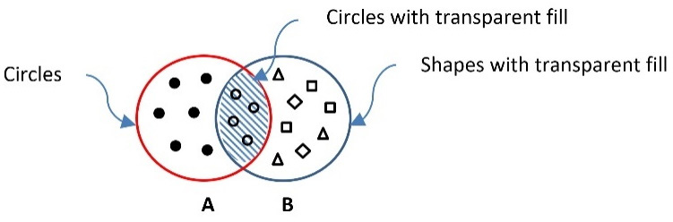
Figure 2.13 – The intersection of the set with circles with the set of all transparent shapes

The intersection of the two sets is highlighted with the grid texture and mathematically written as A∩B or B∩A. Then, we construct Table 2.6, which helps us perform some interesting calculations:

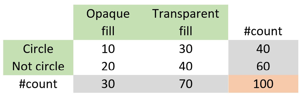
Table 2.6 – The number of shapes by type and fill

First, notice that the total number of items in the table equals 100 (the number of shapes). We can then calculate the following quantities:

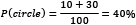
• The probability of getting a circle is
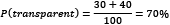
• The probability of getting a transparent fill is
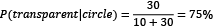
• The probability of getting a transparent fill when the shape is a circle is
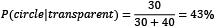
• The probability of getting a circle when the fill is transparent is

The symbol signifies conditional probability. Based on these numbers, we can identify a relationship between the probabilities:

The previous equation suggests that if the probability P(transparent|circle) is unknown, we can use the others to calculate it. We can also generalize the equation as follows:

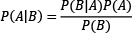
Exploring the different elements, we reach the famous formula known as Bayes’ theorem, which is fundamental in information theory and ML:

The exercise in Table 2.6 was just an example to introduce the fundamental reasoning behind the theorem; all quantities are available to calculate the corresponding probabilities. However, this is not the case in most practical problems, and this is where Bayes’ theorem comes in handy. For example, consider the following situation: you are concerned that you have a severe illness and decide to go to the hospital for a test. Sadly, the test is positive. According to your doctor, the test has 99% reliability; for 99 out of 100 sick people, the test is positive, and for 99 out of 100 healthy people, the test is negative. So, what is the probability of you having the disease? Most people logically answer 99%, but this is not true. The Bayesian reasoning tells us why.

We have a population of 10,000 people, and according to statistics, 1% (so, 100 people) of this population has the illness. Therefore, based on a 99% reliability, this is what we know:

• Of the 100 sick subjects, 99 times (99%), the test is positive, and 1 is negative (1% and therefore wrong).
• Of the 9,900 healthy subjects, 99 times (1%), the test is positive, and 9,801 is negative (99% and therefore correct).

As before, we construct Table 2.7, which helps us with the calculations:

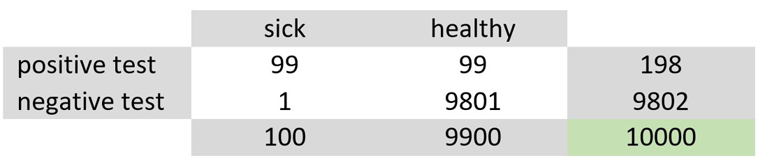
Table 2.7 – The number of people by health condition and test outcome

At first glance, the numbers suggest that there is a non-negligible likelihood that you are healthy and that the test is wrong (99/10000≈1%). Next, we are looking for the probability of being sick given a positive test. So, let’s see the following:

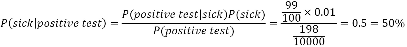
This percentage is much smaller than the 99% initially suggested by most people. What is the catch here? The probability P(sick) in the equation is not something we know exactly, as in the case of the shapes in the previous example. It’s merely our best estimate on the problem, which is called prior probability. The knowledge we have before delving into the problem is the hardest part of the equation to figure out.

Conversely, the probability P(sick|positive test) represents our knowledge after solving the problem, which is called posterior probability. If, for example, you retook the test and this showed to be positive, the previous posterior probability becomes your new prior one – the new posterior increases, which makes sense. Specifically, you did two tests, and both were positive.

Takeaway

Bayesian reasoning tells us how to update our prior beliefs in light of new evidence. As new evidence surfaces, your predictions become better and better.

Remember this discussion the next time you read an article on the internet about an illness! Of course, you always need to interpret the percentages in the proper context. But let’s return to the spam filtering problem and see how to apply the theorem in this case.

Introducing the Naïve Bayes algorithm

Naïve Bayes is a classification algorithm based on Bayes’ theorem. We already know that the features in the emails are the actual words, so we are interested in calculating each posterior probability P(spam|word) with the help of the following theorem:

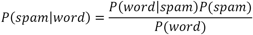
where .

Flipping a coin once gives a ½ probability of getting tails. The probability of getting tails two consecutive times is ¼, as P(tail first time)P(tail second time)=(½)(½)=¼. Thus, repeating the previous calculation for each word in the email (N words in total), we just need to multiply their individual probabilities:

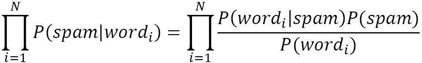
As with the SVM, it is straightforward to incorporate Naïve Bayes using sklearn. In the following code, we use the algorithm’s MultinomialNB implementation to suit the discrete values (word counts) used as features better:

from sklearn import naive_bayes
# Create the classifier.
nb_classifier = naive_bayes.MultinomialNB(alpha=1.0)
# Fit the classifier with the train data.
nb_classifier.fit(train_data_features.toarray(), train_class)
# Get the classification score of the train data.
nb_classifier.score(train_data_features.toarray(), train_class)
>> 0.8641791044776119

Next, we incorporate the test set:

# Get the classification score of the test data.
nb_classifier.score(test_data_features.toarray(), test_class)
>> 0.8571428571428571

The outcome suggests that the performance of this classifier is inferior. Also, notice the result on the actual training set, which is low and very close to the performance on the test set. These numbers are another indication that the created model is not working very well.

Clarifying important key points

Before concluding this section, we must clarify some points concerning the Naïve Bayes algorithm. First of all, it assumes that a particular feature in the data is unrelated to the presence of any other feature. In our case, the assumption is that the words in an email are conditionally independent of each other, given that the type of the email is known (either spam or ham). For example, encountering the word deep does not suggest the presence or the absence of the word learning in the same email. Of course, we know that this is not the case, and many words tend to appear in groups (remember the discussion about n-grams). Most of the time, the assumption of independence of words is false and naive, and this is what the algorithm’s name stems from. In reality, of course, the assumption of independence allows us to solve many practical problems.

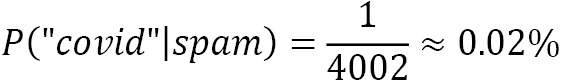
Another issue is when a word appears in the ham emails but is not present in the spam ones (say, covid). Then, according to the algorithm, its conditional probability is zero, P(“covid”|spam) = 0, which is rather inconvenient since we are going to multiply it with the other probabilities (making the outcome equal to zero). This situation is often known as the zero-frequency problem. The solution is to apply smoothing techniques such as Laplace smoothing, where the word count starts at 1 instead of 0.

Let’s see an example of this problem. In a corpus of 10,000 emails, 6,000 are ham and 4,000 are spam. The word heritage appears in 37 emails of the first category and 453 of the second one. Its conditional probabilities are the following:

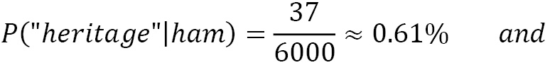
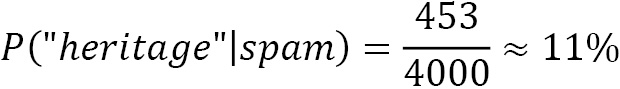
Moreover:

For an email that contains both words (heritage and covid), we need to multiply their individual probabilities (the symbol “…” signifies the other factors in the multiplication):

To overcome this problem, we apply Laplace smoothing, adding 1 in the numerator and 2 in the denominator. As a result, the smoothed probabilities now become the following:

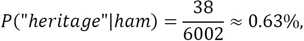
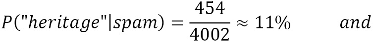
Notice that Laplace smoothing is a hyperparameter that you can specify before running the classification algorithm. For example, in the Python code used in the previous section, we constructed the MultinomialNB classifier using the alpha=1.0 smoothing parameter in the argument list.

This section incorporated two well-known classification algorithms, the SVM and Naïve Bayes, and implemented two versions of a spam detector. We saw how to acquire and prepare the text data for training models, and we got a better insight into the trade-offs while adjusting the hyperparameters of the classifiers. Finally, this section provided some preliminary performance scores, but we still lack adequate knowledge to assess the two models. This discussion is the topic of the next section.

The standard approach for any ML problem incorporates different classification algorithms and examines which works best. Previously, we used two classification methods for the spam filtering problem, but our job is not done yet; we need to evaluate their performance in more detail. Therefore, this section presents a deeper discussion on standard evaluation metrics for this task.

Calculating accuracy

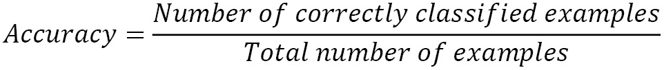
If you had to choose only one of the two created models for a production system, which would that be? The spontaneous answer is to select the one with the highest accuracy. The argument is that the algorithm with the highest number of correct classifications should be the right choice. Although this is not far from the truth, it is not always the case. Accuracy is the percentage of correctly classified examples by an algorithm divided by the total number of examples:

Suppose that a dataset consists of 1,000 labeled emails. Table 2.8 shows a possible outcome after classifying the samples:

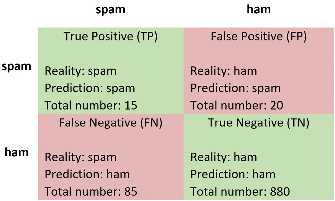
Table 2.8 – A confusion matrix after classifying 1,000 emails

Each cell contains information about the following:

• The correct label of the sample (Reality)
• The classification result (Prediction)
• Total number of samples

For example, 85 emails are labeled as ham, but they are, in reality, spam (in the bottom-left cell). This table, known as a confusion matrix, is used to evaluate the performance of a classification model and provide a better insight into the types of error. Ideally, we would prefer all model predictions to appear in the main diagonal (True Positive and True Negative). From the matrix, we can immediately observe that the dataset is imbalanced, as it contains 100 spam emails and 900 ham ones.

We can rewrite the formula for accuracy based on the previous information as follows:

89.5% of accuracy doesn’t seem that bad, but a closer look at the data reveals a different picture. Out of the 100 spam emails (TPs + FNs), only 15 are identified correctly, and the other 85 are labeled as ham emails. Alas, this score is a terrible result indeed! To assess the performance of a model correctly, we need to make this analysis and consider the type of errors that are most important within the task. Is it better to have a strict model that can block a legitimate email for the sake of fewer spam ones (increased FPs)? Or is it preferable to have a lenient model that doesn’t block most ham emails but allows more undetected spam in your mailbox (increased FNs)?

Similar questions arise in all ML problems and generally in many real-world situations. For example, wrong affirmative decisions (FPs) in a fire alarm system are preferable to wrong negative ones (FNs). In the first case, we get a false alert of a fire that didn’t occur. Conversely, declaring innocent a guilty prisoner implies higher FNs, which is preferable to finding guilty an innocent one (higher FPs). Accuracy is a good metric when the test data is balanced and the classes are equally important.

In the following Python code, we calculate the accuracy for a given test set:

from sklearn import metrics
# Get the predicted classes.
test_class_pred = nb_classifier.predict(test_data_features.toarray())
# Calculate the accuracy on the test set.
metrics.accuracy_score(test_class, test_class_pred)
>> 0.8571428571428571

Accuracy is a prominent and easy-to-interpret metric for any ML problem. As already discussed, however, it poses certain limitations. The following section focuses on metrics that shed more light on the error types.

Calculating precision and recall

Aligned with the previous discussion, we can introduce two evaluation metrics: precision and recall. First, precision tells us the proportion of positive identifications that are, in reality, correct, and it’s defined as the following (with the numbers as taken from Table 2.8):

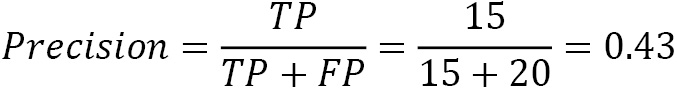
In this case, only 43% of all emails identified as spam are actually spam. The same percentage in a medical screening test suggests that 43% of patients classified as having the disease genuinely have it. A model with zero FPs has a precision equal to 1.

Recall, on the other hand, tells us the proportion of the actual positives that are identified correctly, and it’s defined as the following:

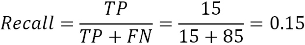
Here, the model identifies only 15% of all spam emails. Ditto, 15% of the patients with a disease are classified as having the disease, while 85 sick people remain undiagnosed. A model with zero FNs has a recall equal to 1. Improving precision often deteriorates recall and vice versa (remember the discussion on strict and lenient models in the previous section).

We can calculate both metrics in the following code using the Naïve Bayes model:

# Calculate the precision on the test set.
metrics.precision_score(test_class, test_class_pred)
>> 0.8564814814814815

After calculating precision, we do the same for recall:

# Calculate the recall on the test set.
metrics.recall_score(test_class, test_class_pred)
>> 1.0

Notice that in this case, recall is equal to 1.0, suggesting the model captured all spam emails. Equipped with the necessary understanding of these metrics, we can continue on the same path and introduce another typical score.

Calculating the F-score

We can combine precision and recall in one more reliable F-score metric: their harmonic mean, given by the following equation:

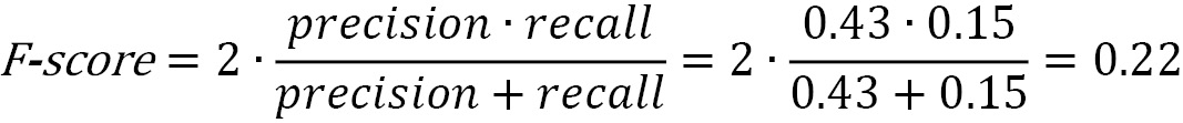
When precision and recall reach their perfect score (equal to 1), the F-score becomes 1. In the following code, we calculate the F-score comparing the actual class labels in the test set and the ones predicted by the model:

# Calculate the F-score on the test set.
metrics.f1_score(test_class, test_class_pred)
>> 0.9226932668329177

As we can observe, the Naïve Bayes model has an F-score equal to 0.92. Running the same code for the SVM case gives an F-score of 0.93.

The following section discusses another typical evaluation metric.

Creating ROC and AUC

When the classifier returns some kind of confidence score for each prediction, we can use another technique for evaluating performance called the Receiver Operator Characteristic (ROC) curve. A ROC curve is a graphical plot that shows the model’s performance at all classification thresholds. It utilizes two rates, namely the True Positive Rate (TPR), the same as recall, and the False Positive Rate (FPR), defined as the following:

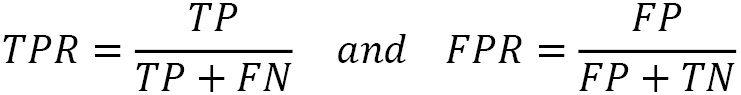
The benefit of ROC curves is that they help us visually identify the trade-offs between the TPR and FPR. In this way, we can find which classification threshold better suits the problem under study. For example, we need to ensure that no important email is lost during spam detection (and consequently, label more spam emails as ham). But, conversely, we must ascertain that all ill patients are diagnosed (and consequently, label more healthy individuals as sick). These two cases require a different trade-off between the TPR and FPR.

Let’s see how to create a ROC curve plot in Table 2.9 using a simplified example with 10 emails and 7 thresholds:

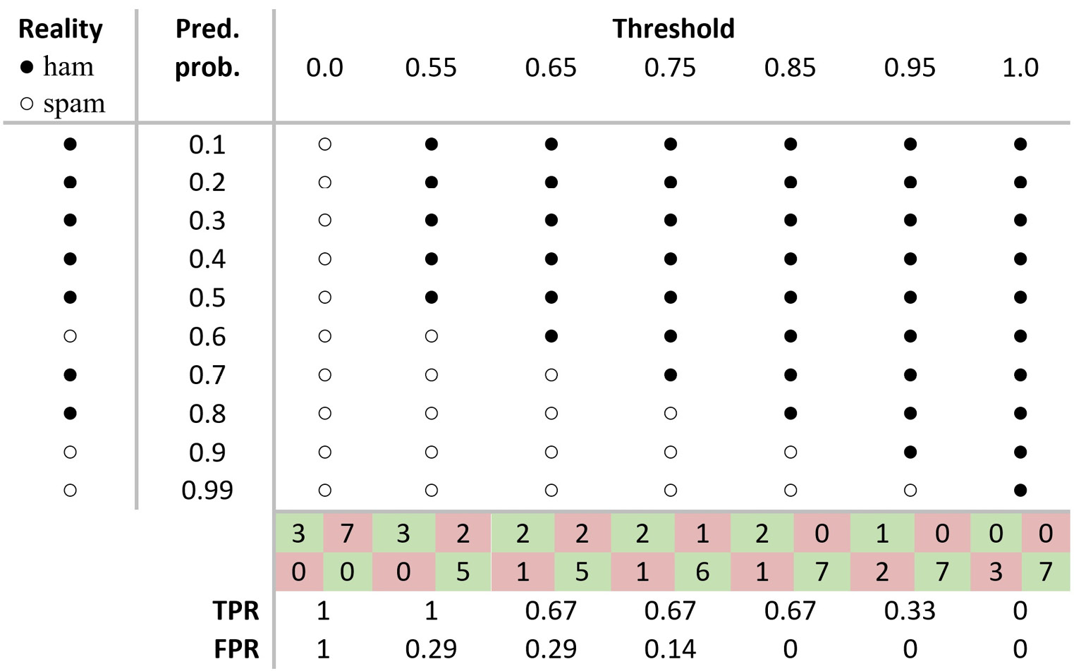
Table 2.9 – Calculating the TPR and FPR scores for different thresholds

For each sample in the first column of the table, we get a prediction score (probability) in the second one. Then, we compare this score with the thresholds. If the score exceeds the threshold, the example is labeled as ham. Observe the first sample in the table, which is, in reality, ham (represented by a black dot). The model outputs a prediction probability equal to 0.1, which labels the sample as ham for all thresholds except the first one. Repeating the same procedure for all samples, we can extract the confusion matrix in each case and calculate the TPR and FPR. Notice that for a threshold equal to 0, the two metrics are equal to 1. Conversely, if the threshold is 1, the metrics are equal to 0.

Figure 2.14 shows the different possible results of this process. The grayed area in these plots, called the Area Under the ROC Curve (AUC), is related to the quality of our model; the higher its surface, the better it is:

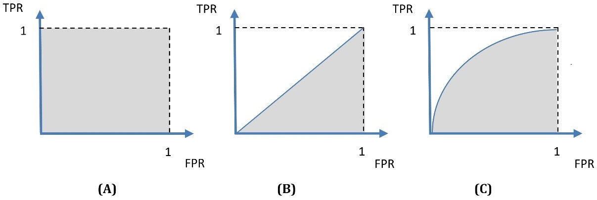
Figure 2.14 – Different ROC curves and their corresponding AUCs

Interesting fact

Radar engineers first developed the ROC curve during World War II for detecting enemy objects on battlefields.

A in Figure 2.14 represents the ideal situation, as there are no classification errors. B in Figure 2.14 represents a random classifier, so if you end up with a similar plot, you can flip a coin and decide on the outcome, as your ML model won’t provide any additional value. However, most of the time, we obtain plots similar to C in Figure 2.14. To summarize, the benefit of ROC curves is twofold:

• We can directly compare different models to find the one with a higher AUC.
• We can specify which TPR and FPR combination offers good classification performance for a specific model.

We can now apply the knowledge about the ROC and AUC to the spam detection problem. In the following code, we perform the necessary steps to create the ROC curves for the two models:

# Create and plot the ROC curves.
nb_disp = metrics.plot_roc_curve(nb_classifier, test_data_features.toarray(), test_class)
svm_disp = metrics.plot_roc_curve(svm_classifier, test_data_features.toarray(), test_class, ax=nb_disp.ax_)
svm_disp.figure_.suptitle("ROC curve comparison")

Figure 2.15 shows the output of this process:

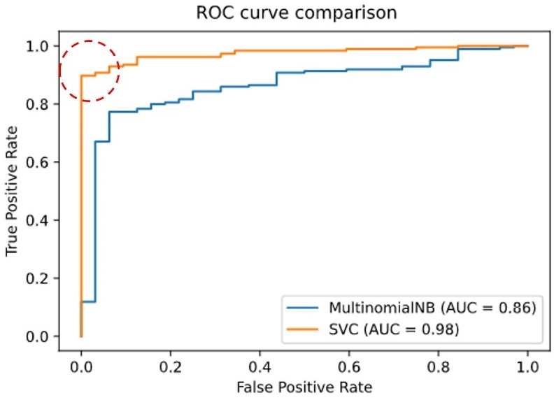
Figure 2.15 – The AUC for the SVM and the Naïve Bayes model

According to the figure, the AUC is 0.98 for the SVM and 0.87 for Naïve Bayes. All results so far corroborate our initial assumption of the superiority of the SVM model. Finally, the best trade-off between the TPR and FPR lies in the points inside the dotted circle. For these points, the TPR is close to 1.0 and the FPR close to 0.0.

Creating precision-recall curves

Before concluding the chapter, let’s cover one final topic. ROC curves can sometimes perform too optimistically with imbalanced datasets. For example, using the TN factor during the FPR calculation can skew the results; look at the disproportional value of TN in Table 2.8. Fortunately, this factor is not part of the precision or recall formulas. The solution, in this case, is to generate another visualization called the Precision-Recall curve. Let’s see how to create the curves for the Naïve Bayes predictions:

1. Initially, we extract the ROC:

   # Obtain the scores for each prediction.
   probs = nb_classifier.predict_proba(test_data_features.toarray())
   test_score = probs[:, 1]
   # Compute the Receiver Operating Characteristic.
   fpr, tpr, thresholds = metrics.roc_curve(test_class, test_score)
   # Compute Area Under the Curve.
   roc_auc = metrics.auc(fpr, tpr)
   # Create the ROC curve.
   rc_display = metrics.RocCurveDisplay(fpr=fpr, tpr=tpr, roc_auc=roc_auc, estimator_name='MultinomialNB')

2. Let’s use the same predictions to create the precision-recall curves:

   # Create the precision recall curves.
   precision, recall, thresholds = metrics.precision_recall_curve(test_class, test_score)
   ap = metrics.average_precision_score(test_class, test_score)
   pr_display = metrics.PrecisionRecallDisplay(precision=precision, recall=recall, average_precision=ap, estimator_name='MultinomialNB')

3. We can combine and show both plots in one:

   # Plot the curves.
   fig, (ax1, ax2) = plt.subplots(1, 2, figsize=(10, 5))
   rc_display.plot(ax=ax1)
   pr_display.plot(ax=ax2)

The output in Figure 2.16 presents the ROC and precision-recall curves side by side:

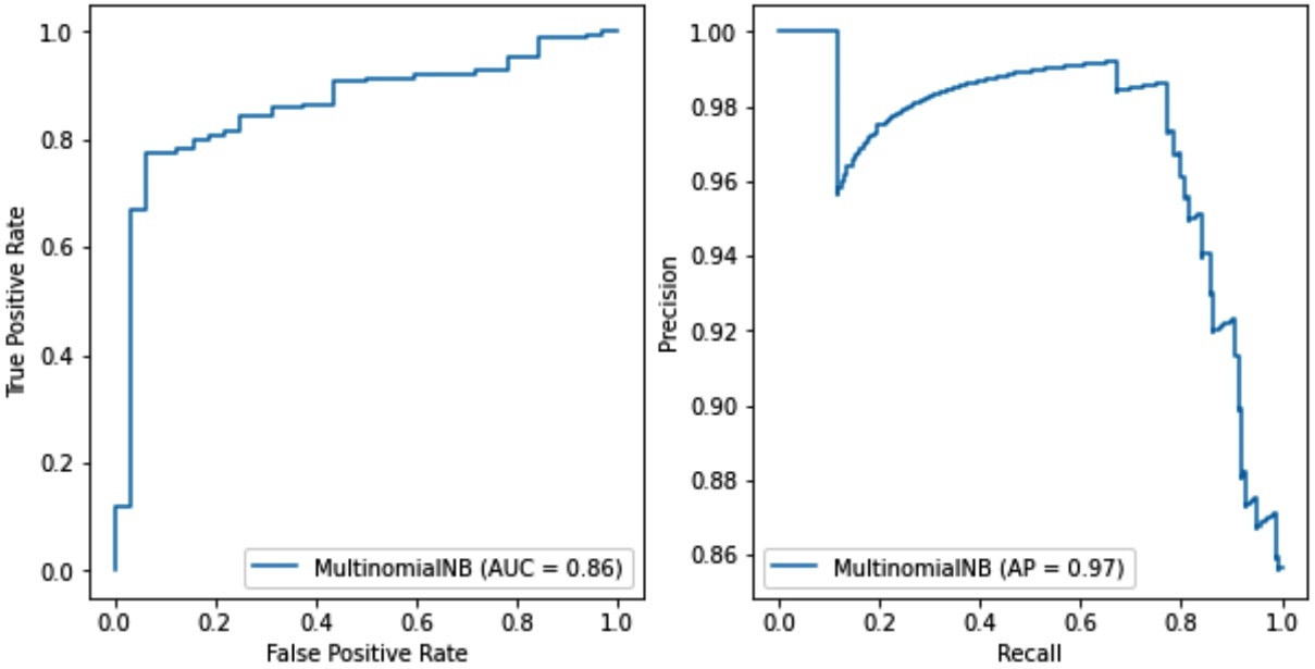
Figure 2.16 – The ROC curve (left) versus the precision-recall curve (right) for the Naïve Bayes model

Both plots summarize the trade-offs between the rates on the x and y axes using different probability thresholds. In the right plot, the average precision (AP) is 0.97 for the Naïve Bayes model and 0.99 for the SVM (not shown). Therefore, we do not observe any mismatch between the ROC and the precision-recall curves concerning which model is better. The SVM is the definite winner! One possible scenario when using imbalance sets is that the TN factor can affect the choice of the best model. In this case, we must scrutinize both types of curves to understand the models’ performance and the differences between the classifiers. The takeaway is that a metric’s effectiveness depends on the specific application and should always be examined from this perspective.

This chapter introduced many fundamental concepts, methods, and techniques for ML in the realm of text data. Then, we had the opportunity to apply this knowledge to solve a spam detection problem by incorporating two supervised ML algorithms. The content unfolded as a pipeline of different tasks, including text preprocessing, text representation, and classification. Comparing the performance of different models constitutes an integral part of this pipeline, and in the last part of the chapter, we dealt with explaining the relevant metrics. Hopefully, you should be able to apply the same process to any similar problem in the future.

Concluding the chapter, we need to make it clear that spam detection in modern deployments is not just a static binary classifier but resembles an adversarial situation. One party constantly tries to modify the messages to avoid detection, while the other party constantly tries to adapt its detection mechanisms to the new threat.

The next chapter expands on the ideas introduced in this chapter but focuses on more advanced techniques to perform topic classification.