


Note
Learning Objectives
We will start our journey by understanding the power of Python to manipulate and visualize data, creating useful analysis.
By the end of this chapter, you will be able to:
Use all components of the Python data science stack
Manipulate data using pandas DataFrames
Create simple plots using pandas and Matplotlib
The Python data science stack is an informal name for a set of libraries used together to tackle data science problems. There is no consensus on which libraries are part of this list; it usually depends on the data scientist and the problem to be solved. We will present the libraries most commonly used together and explain how they can be used.
In this chapter, we will learn how to manipulate tabular data with the Python data science stack. The Python data science stack is the first stepping stone to manipulate large datasets, although these libraries are not commonly used for big data themselves. The ideas and the methods that are used here will be very helpful when we get to large datasets.
One of the main reasons Python is a powerful programming language is the libraries and packages that come with it. There are more than 130,000 packages on the Python Package Index (PyPI) and counting! Let's explore some of the libraries and packages that are part of the data science stack.
The components of the data science stack are as follows:
NumPy: A numerical manipulation package
pandas: A data manipulation and analysis library
SciPy library: A collection of mathematical algorithms built on top of NumPy
Matplotlib: A plotting and graph library
IPython: An interactive Python shell
Jupyter notebook: A web document application for interactive computing
The combination of these libraries forms a powerful tool set for handling data manipulation and analysis. We will go through each of the libraries, explore their functionalities, and show how they work together. Let's start with the interpreters.
The IPython shell (https://ipython.org/) is an interactive Python command interpreter that can handle several languages. It allows us to test ideas quickly rather than going through creating files and running them. Most Python installations have a bundled command interpreter, usually called the shell, where you can execute commands iteratively. Although it's handy, this standard Python shell is a bit cumbersome to use. IPython has more features:
Input history that is available between sessions, so when you restart your shell, the previous commands that you typed can be reused.
Using Tab completion for commands and variables, you can type the first letters of a Python command, function, or variable and IPython will autocomplete it.
Magic commands that extend the functionality of the shell. Magic functions can enhance IPython functionality, such as adding a module that can reload imported modules after they are changed in the disk, without having to restart IPython.
Syntax highlighting.
Getting started with the Python shell is simple. Let's follow these steps to interact with the IPython shell:
To start the Python shell, type the ipython command in the console:
> ipython
In [1]:
The IPython shell is now ready and waiting for further commands. First, let's do a simple exercise to solve a sorting problem with one of the basic sorting methods, called straight insertion.
In the IPython shell, copy-paste the following code:
import numpy as np

vec = np.random.randint(0, 100, size=5)
print(vec)
Now, the output for the randomly generated numbers will be similar to the following:
[23, 66, 12, 54, 98, 3]
Use the following logic to print the elements of the vec array in ascending order:
for j in np.arange(1, vec.size):
    v = vec[j]
    i = j
    while i > 0 and vec[i-1] > v:
        vec[i] = vec[i-1]
        i = i - 1
    vec[i] = v
Use the print(vec) command to print the output on the console:
[3, 12, 23, 54, 66, 98]
Now modify the code. Instead of creating an array of 5 elements, change its parameters so it creates an array with 20 elements, using the up arrow to edit the pasted code. After changing the relevant section, use the down arrow to move to the end of the code and press Enter to execute it.
Notice the number on the left, indicating the instruction number. This number always increases. We attributed the value to a variable and executed an operation on that variable, getting the result interactively. We will use IPython in the following sections.
The Jupyter notebook (https://jupyter.org/) started as part of IPython but was separated in version 4 and extended, and lives now as a separate project. The notebook concept is based on the extension of the interactive shell model, creating documents that can run code, show documentation, and present results such as graphs and images.
Jupyter is a web application, so it runs in your web browser directly, without having to install separate software, and enabling it to be used across the internet. Jupyter can use IPython as a kernel for running Python, but it has support for more than 40 kernels that are contributed by the developer community.
Note
A kernel, in Jupyter parlance, is a computation engine that runs the code that is typed into a code cell in a notebook. For example, the IPython kernel executes Python code in a notebook. There are kernels for other languages, such as R and Julia.
It has become a de facto platform for performing operations related to data science from beginners to power users, and from small to large enterprises, and even academia. Its popularity has increased tremendously in the last few years. A Jupyter notebook contains both the input and the output of the code you run on it. It allows text, images, mathematical formulas, and more, and is an excellent platform for developing code and communicating results. Because of its web format, notebooks can be shared over the internet. It also supports the Markdown markup language and renders Markdown text as rich text, with formatting and other features supported.
As we've seen before, each notebook has a kernel. This kernel is the interpreter that will execute the code in the cells. The basic unit of a notebook is called a cell. A cell is a container for either code or text. We have two main types of cells:
Code cell
Markdown cell
A code cell accepts code to be executed in the kernel, displaying the output just below it. A Markdown cell accepts Markdown and will parse the text in Markdown to formatted text when the cell is executed.
Let's run the following exercise to get hands-on experience in the Jupyter notebook.
The fundamental component of a notebook is a cell, which can accept code or text depending on the mode that is selected.
Let's start a notebook to demonstrate how to work with cells, which have two states:
Edit mode
Run mode
When in edit mode, the contents of the cell can be edited, while in run mode, the cell is ready to be executed, either by the kernel or by being parsed to formatted text.
You can add a new cell by using the Insert menu option or using a keyboard shortcut, Ctrl + B. Cells can be converted between Markdown mode and code mode again using the menu or the Y shortcut key for a code cell and M for a Markdown cell.
To execute a cell, click on the Run option or use the Ctrl + Enter shortcut.
Let's execute the following steps to demonstrate how to start to execute simple programs in a Jupyter notebook.
Working with a Jupyter notebook for the first time can be a little confusing, but let's try to explore its interface and functionality. The reference notebook for this exercise is provided on GitHub.
Now, start a Jupyter notebook server and work on it by following these steps:
To start the Jupyter notebook server, run the following command on the console:
> jupyter notebook
After successfully running or installing Jupyter, open a browser window and navigate to http://localhost:8888 to access the notebook.
You should see a notebook similar to the one shown in the following screenshot:
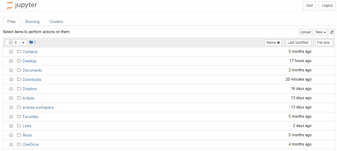
Figure 1.1: Jupyter notebook
After that, from the top-right corner, click on New and select Python 3 from the list.
A new notebook should appear. The first input cell that appears is a Code cell. The default cell type is Code. You can change it via the Cell Type option located under the Cell menu:
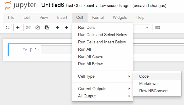
Figure 1.2: Options in the cell menu of Jupyter
Now, in the newly generated Code cell, add the following arithmetic function in the first cell:
In []: x = 2
       print(x*2)
Out []: 4
Now, add a function that returns the arithmetic mean of two numbers, and then execute the cell:
In []: def mean(a,b):
       return (a+b)/2
Let's now use the mean function and call the function with two values, 10 and 20. Execute this cell. What happens? The function is called, and the answer is printed:
In []: mean(10,20)
Out[]: 15.0
We need to document this function. Now, create a new Markdown cell and edit the text in the Markdown cell, documenting what the function does:
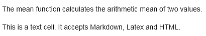
Figure 1.3: Markdown in Jupyter
Then, include an image from the web. The idea is that the notebook is a document that should register all parts of analysis, so sometimes we need to include a diagram or graph from other sources to explain a point.
Now, finally, include the mathematical expression in LaTex in the same Markdown cell:
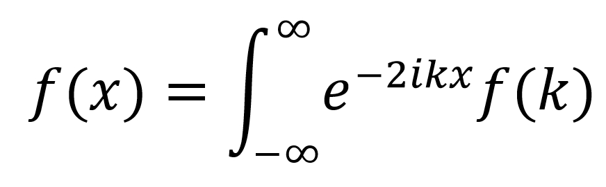
Figure 1.4: LaTex expression in Jupyter Markdown
As we will see in the rest of the book, the notebook is the cornerstone of our analysis process. The steps that we just followed illustrate the use of different kinds of cells and the different ways we can document our analysis.
Both IPython and Jupyter have a place in the analysis workflow. Usually, the IPython shell is used for quick interaction and more data-heavy work, such as debugging scripts or running asynchronous tasks. Jupyter notebooks, on the other hand, are great for presenting results and generating visual narratives with code, text, and figures. Most of the examples that we will show can be executed in both, except the graphical parts.
IPython is capable of showing graphs, but usually, the inclusion of graphs is more natural in a notebook. We will usually use Jupyter notebooks in this book, but the instructions should also be applicable to IPython notebooks.
Let's demonstrate common Python development in IPython and Jupyter. We will import NumPy, define a function, and iterate the results:
Open the python_script_student.py file in a text editor, copy the contents to a notebook in IPython, and execute the operations.
Copy and paste the code from the Python script into a Jupyter notebook.
Now, update the values of the x and c constants. Then, change the definition of the function.
We now know how to handle functions and change function definitions on the fly in the notebook. This is very helpful when we are exploring and discovering the right approach for some code or an analysis. The iterative approach allowed by the notebook can be very productive in prototyping and faster than writing code to a script and executing that script, checking the results, and changing the script again.
NumPy (http://www.numpy.org) is a package that came from the Python scientific computing community. NumPy is great for manipulating multidimensional arrays and applying linear algebra functions to those arrays. It also has tools to integrate C, C++, and Fortran code, increasing its performance capabilities even more. There are a large number of Python packages that use NumPy as their numerical engine, including pandas and scikit-learn. These packages are part of SciPy, an ecosystem for packages used in mathematics, science, and engineering.
To import the package, open the Jupyter notebook used in the previous activity and type the following command:
import numpy as np
The basic NumPy object is ndarray, a homogeneous multidimensional array, usually composed of numbers, but it can hold generic data. NumPy also includes several functions for array manipulation, linear algebra, matrix operations, statistics, and other areas. One of the ways that NumPy shines is in scientific computing, where matrix and linear algebra operations are common. Another strength of NumPy is its tools that integrate with C++ and FORTRAN code. NumPy is also heavily used by other Python libraries, such as pandas.
SciPy (https://www.scipy.org) is an ecosystem of libraries for mathematics, science, and engineering. NumPy, SciPy, scikit-learn, and others are part of this ecosystem. It is also the name of a library that includes the core functionality for lots of scientific areas.
Matplotlib (https://matplotlib.org) is a plotting library for Python for 2D graphs. It's capable of generating figures in a variety of hard-copy formats for interactive use. It can use native Python data types, NumPy arrays, and pandas DataFrames as data sources. Matplotlib supports several backend—the part that supports the output generation in interactive or file format. This allows Matplotlib to be multiplatform. This flexibility also allows Matplotlib to be extended with toolkits that generate other kinds of plots, such as geographical plots and 3D plots.
The interactive interface for Matplotlib was inspired by the MATLAB plotting interface. It can be accessed via the matplotlib.pyplot module. The file output can write files directly to disk. Matplotlib can be used in scripts, in IPython or Jupyter environments, in web servers, and in other platforms. Matplotlib is sometimes considered low level because several lines of code are needed to generate a plot with more details. One of the tools that we will look at in this book that plots graphs, which are common in analysis, is the Seaborn library, one of the extensions that we mentioned before.
To import the interactive interface, use the following command in the Jupyter notebook:
import matplotlib.pyplot as plt
To have access to the plotting capabilities. We will show how to use Matplotlib in more detail in the next chapter.
Pandas (https://pandas.pydata.org) is a data manipulation and analysis library that's widely used in the data science community. Pandas is designed to work with tabular or labeled data, similar to SQL tables and Excel files.
We will explore the operations that are possible with pandas in more detail. For now, it's important to learn about the two basic pandas data structures: the series, a unidimensional data structure; and the data science workhorse, the bi-dimensional DataFrame, a two-dimensional data structure that supports indexes.
Data in DataFrames and series can be ordered or unordered, homogeneous, or heterogeneous. Other great pandas features are the ability to easily add or remove rows and columns, and operations that SQL users are more familiar with, such as GroupBy, joins, subsetting, and indexing columns. Pandas is also great at handling time series data, with easy and flexible datetime indexing and selection.
Let's import pandas into the Jupyter notebook from the previous activity with the following command:
import pandas as pd
We will demonstrate the main operations for data manipulation using pandas. This approach is used as a standard for other data manipulation tools, such as Spark, so it's helpful to learn how to manipulate data using pandas. It's common in a big data pipeline to convert part of the data or a data sample to a pandas DataFrame to apply a more complex transformation, to visualize the data, or to use more refined machine learning models with the scikit-learn library. Pandas is also fast for in-memory, single-machine operations. Although there is a memory overhead between the data size and the pandas DataFrame, it can be used to manipulate large volumes of data quickly.
We will learn how to apply the basic operations:
Read data into a DataFrame
Selection and filtering
Apply a function to data
GroupBy and aggregation
Visualize data from DataFrames
Let's start by reading data into a pandas DataFrame.
Pandas accepts several data formats and ways to ingest data. Let's start with the more common way, reading a CSV file. Pandas has a function called read_csv, which can be used to read a CSV file, either locally or from a URL. Let's read some data from the Socrata Open Data initiative, a RadNet Laboratory Analysis from the U.S. Environmental Protection Agency (EPA), which lists the radioactive content collected by the EPA.
How can an analyst start data analysis without data? We need to learn how to get data from an internet source into our notebook so that we can start our analysis. Let's demonstrate how pandas can read CSV data from an internet source so we can analyze it:
Import pandas library.
import pandas as pd
Read the Automobile mileage dataset, available at this URL: https://github.com/TrainingByPackt/Big-Data-Analysis-with-Python/blob/master/Lesson01/imports-85.data. Convert it to csv.
Use the column names to name the data, with the parameter names on the read_csv function.
Sample code : df = pd.read_csv("/path/to/imports-85.csv", names = columns)Use the function read_csv from pandas and show the first rows calling the method head on the DataFrame:
import pandas as pd
df = pd.read_csv("imports-85.csv")
df.head()
The output is as follows:

Figure 1.5: Entries of the Automobile mileage dataset
Pandas can read more formats:
JSON
Excel
HTML
HDF5
Parquet (with PyArrow)
SQL databases
Google Big Query
Try to read other formats from pandas, such as Excel sheets.
By data manipulation we mean any selection, transformation, or aggregation that is applied over the data. Data manipulation can be done for several reasons:
To select a subset of data for analysis
To clean a dataset, removing invalid, erroneous, or missing values
To group data into meaningful sets and apply aggregation functions
Pandas was designed to let the analyst do these transformations in an efficient way.
Pandas DataFrames can be sliced similarly to Python lists. For example, to select a subset of the first 10 rows of the DataFrame, we can use the [0:10] notation. We can see in the following screenshot that the selection of the interval [1:3] that in the NumPy representation selects the rows 1 and 2.
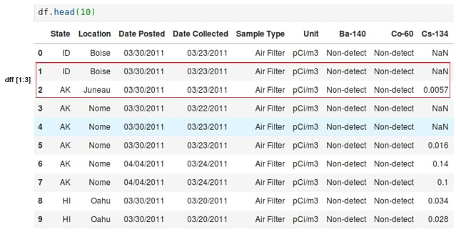
Figure 1.6: Selection in a pandas DataFrame
In the following section, we'll explore the selection and filtering operation in depth.
When performing data analysis, we usually want to see how data behaves differently under certain conditions, such as comparing a few columns, selecting only a few columns to help read the data, or even plotting. We may want to check specific values, such as the behavior of the rest of the data when one column has a specific value.
After selecting with slicing, we can use other methods, such as the head method, to select only a few rows from the beginning of the DataFrame. But how can we select some columns in a DataFrame?
To select a column, just use the name of the column. We will use the notebook. Let's select the cylinders column in our DataFrame using the following command:
df['State']
The output is as follows:
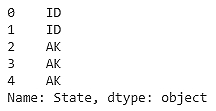
Figure 1.7: DataFrame showing the state
Another form of selection that can be done is filtering by a specific value in a column. For example, let's say that we want to select all rows that have the State column with the MN value. How can we do that? Try to use the Python equality operator and the DataFrame selection operation:
df[df.State == "MN"]
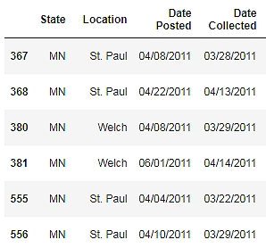
Figure 1.8: DataFrame showing the MN states
More than one filter can be applied at the same time. The OR, NOT, and AND logic operations can be used when combining more than one filter. For example, to select all rows that have State equal to AK and a Location of Nome, use the & operator:
df[(df.State == "AK") & (df.Location == "Nome")]
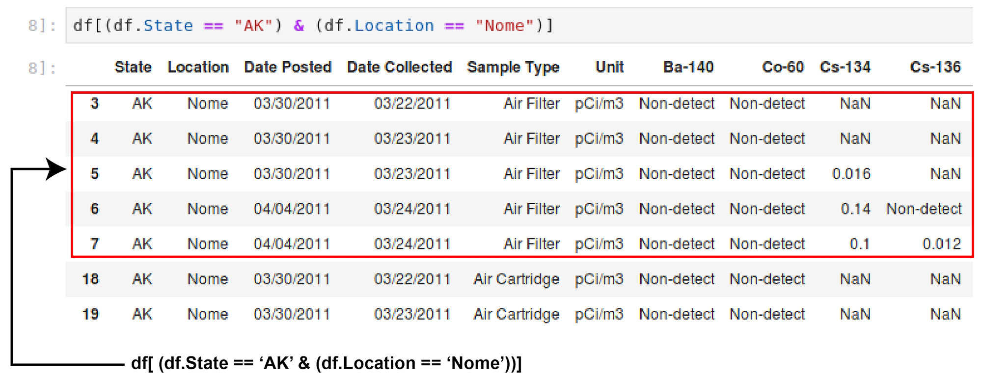
Figure 1.9: DataFrame showing State AK and Location Nome
Another powerful method is .loc. This method has two arguments, the row selection and the column selection, enabling fine-grained selection. An important caveat at this point is that, depending on the applied operation, the return type can be either a DataFrame or a series. The .loc method returns a series, as selecting only a column. This is expected, because each DataFrame column is a series. This is also important when more than one column should be selected. To do that, use two brackets instead of one, and use as many columns as you want to select.
As we saw before, selecting data, separating variables, and viewing columns and rows of interest is fundamental to the analysis process. Let's say we want to analyze the radiation from I-131 in the state of Minnesota:
Import the NumPy and pandas libraries using the following command in the Jupyter notebook:
import numpy as np
import pandas as pd
Read the RadNet dataset from the EPA, available from the Socrata project at https://github.com/TrainingByPackt/Big-Data-Analysis-with-Python/blob/master/Lesson01/RadNet_Laboratory_Analysis.csv:
url = "https://opendata.socrata.com/api/views/cf4r-dfwe/rows.csv?accessType=DOWNLOAD"
df = pd.read_csv(url)
Start by selecting a column using the ['<name of the column>'] notation. Use the State column:
df['State'].head()
The output is as follows:
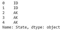
Figure 1.10: Data in the State column
Now filter the selected values in a column using the MN column name:
df[df.State == "MN"]
The output is as follows:
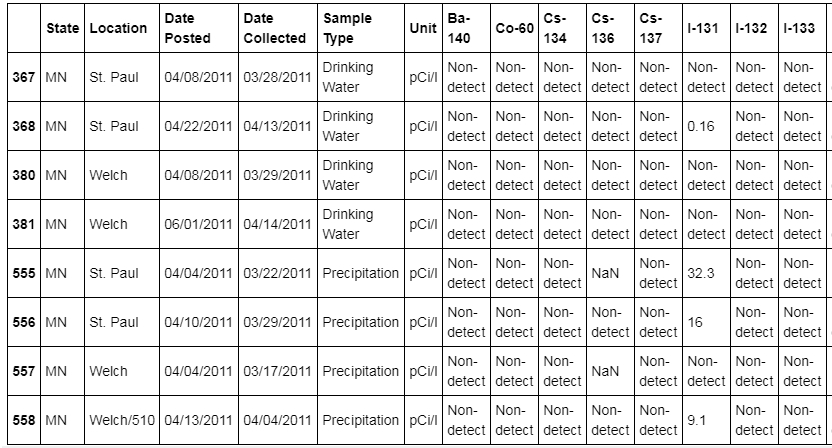
Figure 1.11: DataFrame showing States with MN
Select more than one column per condition. Add the Sample Type column for filtering:
df[(df.State == 'CA') & (df['Sample Type'] == 'Drinking Water')]
The output is as follows:
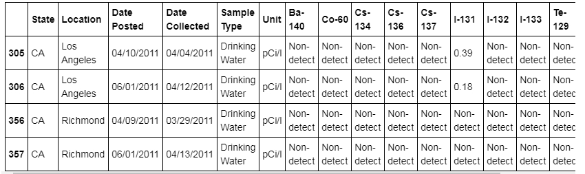
Figure 1.12: DataFrame with State CA and Sample type as Drinking water
Next, select the MN state and the isotope I-131:
df[(df.State == "MN") ]["I-131"]
The output is as follows:
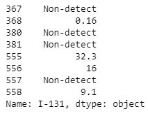
Figure 1.13: Data showing the DataFrame with State Minnesota and Isotope I-131
The radiation in the state of Minnesota with ID 555 is the highest.
We can do the same more easily with the .loc method, filtering by state and selecting a column on the same .loc call:
df_rad.loc[df_rad.State == "MN", "I-131"]
df[['I-132']].head()
The output is as follows:
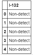
Figure 1.14: DataFrame with I-132
In this exercise, we learned how to filter and select values, either on columns or rows, using the NumPy slice notation or the .loc method. This can help when analyzing data, as we can check and manipulate only a subset of the data instead having to handle the entire dataset at the same time.
Note
The result of the .loc filter is a series and not a DataFrame. This depends on the operation and selection done on the DataFrame and not is caused only by .loc. Because the DataFrame can be understood as a 2D combination of series, the selection of one column will return a series. To make a selection and still return a DataFrame, use double brackets:
df[['I-132']].head()
Data is never clean. There are always cleaning tasks that have to be done before a dataset can be analyzed. One of the most common tasks in data cleaning is applying a function to a column, changing a value to a more adequate one. In our example dataset, when no concentration was measured, the non-detect value was inserted. As this column is a numerical one, analyzing it could become complicated. We can apply a transformation over a column, changing from non-detect to numpy.NaN, which makes manipulating numerical values more easy, filling with other values such as the mean, and so on.
To apply a function to more than one column, use the applymap method, with the same logic as the apply method. For example, another common operation is removing spaces from strings. Again, we can use the apply and applymap functions to fix the data. We can also apply a function to rows instead of to columns, using the axis parameter (0 for rows, 1 for columns).
Before starting an analysis, we need to check for data problems, and when we find them (which is very common!), we have to correct the issues by transforming the DataFrame. One way to do that, for instance, is by applying a function to a column, or to the entire DataFrame. It's common for some numbers in a DataFrame, when it's read, to not be converted correctly to floating-point numbers. Let's fix this issue by applying functions:
Import pandas and numpy library.
Read the RadNet dataset from the U.S. Environmental Protection Agency.
Create a list with numeric columns for radionuclides in the RadNet dataset.
Use the apply method on one column, with a lambda function that compares the Non-detect string.
Replace the text values by NaN in one column with np.nan.
Use the same lambda comparison and use the applymap method on several columns at the same time, using the list created in the first step.
Create a list of the remaining columns that are not numeric.
Remove any spaces from these columns.
Using the selection and filtering methods, verify that the names of the string columns don't have any more spaces.
The spaces in column names can be extraneous and can make selection and filtering more complicated. Fixing the numeric types helps when statistics must be computed using the data. If there is a value that is not valid for a numeric column, such as a string in a numeric column, the statistical operations will not work. This scenario happens, for example, when there is an error in the data input process, where the operator types the information by hand and makes mistakes, or the storage file was converted from one format to another, leaving incorrect values in the columns.
Another common operation in data cleanup is getting the data types right. This helps with detecting invalid values and applying the right operations. The main types stored in pandas are as follows:
float (float64, float32)
integer (int64, int32)
datetime (datetime64[ns, tz])
timedelta (timedelta[ns])
bool
object
category
Types can be set on, read, or inferred by pandas. Usually, if pandas cannot detect what data type the column is, it assumes that is object that stores the data as strings.
To transform the data into the right data types, we can use conversion functions such as to_datetime, to_numeric, or astype. Category types, columns that can only assume a limited number of options, are encoded as the category type.
Transform the data types in our example DataFrame to the correct types with the pandas astype function. Let's use the sample dataset from https://opendata.socrata.com/:
Import the required libraries, as illustrated here:
import numpy as np
import pandas as pd
import matplotlib.pyplot as plt
import seaborn as sns
Read the data from the dataset as follows:
url = "https://opendata.socrata.com/api/views/cf4r-dfwe/rows.csv?accessType=DOWNLOAD"
df = pd.read_csv(url)
Check the current data types using the dtypes function on the DataFrame:
df.dtypes
Use the to_datetime method to convert the dates from string format to datetime format:
df['Date Posted'] = pd.to_datetime(df['Date Posted'])
df['Date Collected'] = pd.to_datetime(df['Date Collected'])
columns = df.columns
id_cols = ['State', 'Location', "Date Posted", 'Date Collected', 'Sample Type', 'Unit']
columns = list(set(columns) - set(id_cols))
columns
The output is as follows:
['Co-60',
 'Cs-136',
 'I-131',
 'Te-129',
 'Ba-140',
 'Cs-137',
 'Cs-134',
 'I-133',
 'I-132',
 'Te-132',
 'Te-129m']
Use Lambda function:
df['Cs-134'] = df['Cs-134'].apply(lambda x: np.nan if x == "Non-detect" else x)
df.loc[:, columns] = df.loc[:, columns].applymap(lambda x: np.nan if x == 'Non-detect' else x)
df.loc[:, columns] = df.loc[:, columns].applymap(lambda x: np.nan if x == 'ND' else x)
Apply the to_numeric method to the list of numeric columns created in the previous activity to convert the columns to the correct numeric types:
for col in columns:
    df[col] = pd.to_numeric(df[col])
Check the types of the columns again. They should be float64 for the numeric columns and datetime64[ns] for the date columns:
df.dypes
Use the astype method to transform the columns that are not numeric to the category type:
df['State'] = df['State'].astype('category')
df['Location'] = df['Location'].astype('category')
df['Unit'] = df['Unit'].astype('category')
df['Sample Type'] = df['Sample Type'].astype('category')
Check the types with the dtype function for the last time:
df.dtypes
The output is as follows:
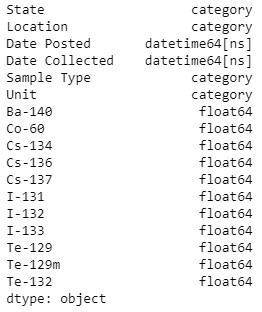
Figure 1.15: DataFrame and its types
Now our dataset looks fine, with all values correctly cast to the right types. But correcting the data is only part of the story. We want, as analysts, to understand the data from different perspectives. For example, we may want to know which state has the most contamination, or the radionuclide that is the least prevalent across cities. We may ask about the number of valid measurements present in the dataset. All these questions have in common transformations that involve grouping data together and aggregating several values. With pandas, this is accomplished with GroupBy. Let's see how we can use it by key and aggregate the data.
After getting the dataset, our analyst may have to answer a few questions. For example, we know the value of the radionuclide concentration per city, but an analyst may be asked to answer: which state, on average, has the highest radionuclide concentration?
To answer the questions posed, we need to group the data somehow and calculate an aggregation on it. But before we go into grouping data, we have to prepare the dataset so that we can manipulate it in an efficient manner. Getting the right types in a pandas DataFrame can be a huge boost for performance and can be leveraged to enforce data consistency— it makes sure that numeric data really is numeric and allows us to execute operations that we want to use to get the answers.
GroupBy allows us to get a more general view of a feature, arranging data given a GroupBy key and an aggregation operation. In pandas, this operation is done with the GroupBy method, over a selected column, such as State. Note the aggregation operation after the GroupBy method. Some examples of the operations that can be applied are as follows:
mean
median
std (standard deviation)
mad (mean absolute deviation)
sum
count
abs
After applying GroupBy, a specific column can be selected and the aggregation operation can be applied to it, or all the remaining columns can be aggregated by the same function. Like SQL, GroupBy can be applied to more than one column at a time, and more than one aggregation operation can be applied to selected columns, one operation per column.
The GroupBy command in Pandas has some options, such as as_index, which can override the standard of transforming grouping key's columns to indexes and leaving them as normal columns. This is helpful when a new index will be created after the GroupBy operation, for example.
Aggregation operations can be done over several columns and different statistical methods at the same time with the agg method, passing a dictionary with the name of the column as the key and a list of statistical operations as values.
Remember that we have to answer the question of which state has, on average, the highest radionuclide concentration. As there are several cities per state, we have to combine the values of all cities in one state and calculate the average. This is one of the applications of GroupBy: calculating the average values of one variable as per a grouping. We can answer the question using GroupBy:
Import the required libraries:
import numpy as np
import pandas as pd
import matplotlib.pyplot as plt
import seaborn as sns
Load the datasets from the https://opendata.socrata.com/:
df = pd.read_csv('RadNet_Laboratory_Analysis.csv')Group the DataFrame using the State column.
df.groupby('State')Select the radionuclide Cs-134 and calculate the average value per group:
df.groupby('State')['Cs-134'].head()Do the same for all columns, grouping per state and applying directly the mean function:
df.groupby('State').mean().head()Now, group by more than one column, using a list of grouping columns.
Aggregate using several aggregation operations per column with the agg method. Use the State and Location columns:
df.groupby(['State', 'Location']).agg({'Cs-134':['mean', 'std'], 'Te-129':['min', 'max']})
After creating an intermediate or final dataset in pandas, we can export the values from the DataFrame to several other formats. The most common one is CSV, and the command to do so is df.to_csv('filename.csv'). Other formats, such as Parquet and JSON, are also supported.
Note
Parquet is particularly interesting, and it is one of the big data formats that we will discuss later in the book.
After finishing our analysis, we may want to save our transformed dataset with all the corrections, so if we want to share this dataset or redo our analysis, we don't have to transform the dataset again. We can also include our analysis as part of a larger data pipeline or even use the prepared data in the analysis as input to a machine learning algorithm. We can accomplish data exporting our DataFrame to a file with the right format:
Import all the required libraries and read the data from the dataset using the following command:
import numpy as np
import pandas as pd

url = "https://opendata.socrata.com/api/views/cf4r-dfwe/rows.csv?accessType=DOWNLOAD"
df = pd.read_csv(url)
Redo all adjustments for the data types (date, numeric, and categorical) in the RadNet data. The type should be the same as in Exercise 6: Aggregation and Grouping Data.
Select the numeric columns and the categorical columns, creating a list for each of them:
columns = df.columns
id_cols = ['State', 'Location', "Date Posted", 'Date Collected', 'Sample Type', 'Unit']
columns = list(set(columns) - set(id_cols))
columns
The output is as follows:
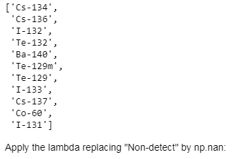
Figure 1.16: List of columns
Apply the lambda function that replaces Non-detect with np.nan:
df['Cs-134'] = df['Cs-134'].apply(lambda x: np.nan if x == "Non-detect" else x)
df.loc[:, columns] = df.loc[:, columns].applymap(lambda x: np.nan if x == 'Non-detect' else x)
df.loc[:, columns] = df.loc[:, columns].applymap(lambda x: np.nan if x == 'ND' else x)
Remove the spaces from the categorical columns:
df.loc[:, ['State', 'Location', 'Sample Type', 'Unit']] = df.loc[:, ['State', 'Location', 'Sample Type', 'Unit']].applymap(lambda x: x.strip())
Transform the date columns to the datetime format:
df['Date Posted'] = pd.to_datetime(df['Date Posted'])
df['Date Collected'] = pd.to_datetime(df['Date Collected'])
Transform all numeric columns to the correct numeric format with the to_numeric method:
for col in columns:
    df[col] = pd.to_numeric(df[col])
Transform all categorical variables to the category type:
df['State'] = df['State'].astype('category')
df['Location'] = df['Location'].astype('category')
df['Unit'] = df['Unit'].astype('category')
df['Sample Type'] = df['Sample Type'].astype('category')
Export our transformed DataFrame, with the right values and columns, to the CSV format with the to_csv function. Exclude the index using index=False, use a semicolon as the separator sep=";", and encode the data as UTF-8 encoding="utf-8":
df.to_csv('radiation_clean.csv', index=False, sep=';', encoding='utf-8')Export the same DataFrame to the Parquet columnar and binary format with the to_parquet method:
df.to_parquet('radiation_clean.prq', index=False)
Pandas can be thought as a data Swiss Army knife, and one thing that a data scientist always needs when analyzing data is to visualize that data. We will go into detail on the kinds of plot that we can apply in an analysis. For now, the idea is to show how to do quick and dirty plots directly from pandas.
The plot function can be called directly from the DataFrame selection, allowing fast visualizations. A scatter plot can be created by using Matplotlib and passing data from the DataFrame to the plotting function. Now that we know the tools, let's focus on the pandas interface for data manipulation. This interface is so powerful that it is replicated by other projects that we will see in this course, such as Spark. We will explain the plot components and methods in more detail in the next chapter.
You will see how to create graphs that are useful for statistical analysis in the next chapter. Focus here on the mechanics of creating plots from pandas for quick visualizations.
To finish up our activity, let's redo all the previous steps and plot graphs with the results, as we would do in a preliminary analysis:
Use the RadNet DataFrame that we have been working with.
Fix all the data type problems, as we saw before.
Create a plot with a filter per Location, selecting the city of San Bernardino, and one radionuclide, with the x-axis as date and the y-axis as radionuclide I-131:
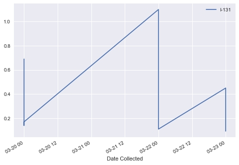
Figure 1.17: Plot of Location with I-131
Create a scatter plot with the concentration of two related radionuclides, I-131 and I-132:
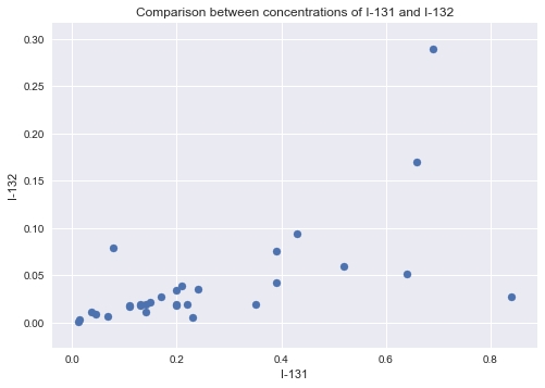
Figure 1.18: Plot of I-131 and I-132
We are getting a bit ahead of ourselves here with the plotting, so we don't need to worry about the details of the plot or how we attribute titles, labels, and so on. The important takeaway here is understanding that we can plot directly from the DataFrame for quick analysis and visualization.
We have learned about the most common Python libraries used in data analysis and data science, which make up the Python data science stack. We learned how to ingest data, select it, filter it, and aggregate it. We saw how to export the results of our analysis and generate some quick graphs.
These are steps done in almost any data analysis. The ideas and operations demonstrated here can be applied to data manipulation with big data. Spark DataFrames were created with the pandas interface in mind, and several operations are performed in a very similar fashion in pandas and Spark, greatly simplifying the analysis process. Another great advantage of knowing your way around pandas is that Spark can convert its DataFrames to pandas DataFrames and back again, enabling analysts to work with the best tool for the job.
Before going into big data, we need to understand how to better visualize the results of our analysis. Our understanding of the data and its behavior can be greatly enhanced if we visualize it using the correct plots. We can draw inferences and see anomalies and patterns when we plot the data.
In the next chapter, we will learn how to choose the right graph for each kind of data and analysis, and how to plot it using Matplotlib and Seaborn.