Overview

This chapter covers the very basic concepts of SQL that will get you started with writing simple commands. By the end of this chapter, you will be able to identify the difference between structured and unstructured data, explain the basic SQL concepts, create tables using the CREATE statement, and insert values into tables using SQL commands.

The vast majority of companies today work with large amounts of data. This could be product information, customer data, client details, employee data, and so on. Most people who are new to working with data will do so using spreadsheets. Software such as Microsoft Excel has many tools for manipulating and analyzing data, but as the volume and complexity of the data you're working with increases, these tools may become inefficient.

A more powerful and controlled way of working with data is to store it in a database and use SQL to access and manipulate it. SQL works extremely well for organized data and can be used very effectively to insert, retrieve, and manipulate data with just a few lines of code. In this chapter, we'll get an introduction to SQL and see how to create databases and tables, as well as how to insert values into them.

For most companies, storing and retrieving data is a day-to-day activity. Based on how data is stored, we can broadly classify data as structured or unstructured. Unstructured data, simply put, is data that is not well-organized. Documents, PDFs, and videos fall into this category—they contain a mixture of different data types (text, images, audio, video, and so on) that have no consistent relationship between them. Media and publishing are examples of industries that deal with unstructured data such as this.

In this book, our focus will be on structured data. Structured data is organized according to a consistent structure. As such, structured data can be easily organized into tables. Thanks to its consistent organization, working with structured data is easier, and it can be processed more effectively. Tables are collections of entities or tuples (rows) and attributes (columns).

For example, consider the following table:

Figure 1.1: An example student's database table

For each row, there is a clear relationship; a given student takes a particular subject and achieves a specific score in that subject. The columns are also known as fields, while the rows are known as records.

Data that is presented in tabular form can be stored in a relational database. Relational databases, as the name suggests, store data that has a certain relationship with another piece of data. A Relational Database Management System (RDBMS) is a system that's used to manage relational data. SQL works very well with relational data. Popular RDBMSs include Microsoft SQL Server, MySQL, and Oracle. Throughout this book, we will be working with MySQL. We can use various SQL commands to work with data in relational databases. We'll have a brief look at them in the next section.

SQL (often pronounced "sequel") stands for Structured Query Language. A query in SQL is constructed using different commands. These commands are classified into what are called sublanguages of SQL. Even if you think you know them already, give this a read to see if these seem more relatable to you. There are five sublanguages in SQL, as follows:

• Data Definition Language (DDL): As the name suggests, the commands that fall under this category work with defining either a table, a database, or anything within. Any command that talks about creating something in SQL is part of DDL. Some examples of such commands are CREATE, ALTER, and DROP.

  The following table shows the DDL commands:

  

Figure 1.2: DDL commands

• Data Manipulation Language (DML): In DML, you do not deal with the containers of data but the data itself. When you must update the data itself, or perform calculations or operations on it, you use the DML. The commands that form part of this language (or sublanguage) include INSERT, UPDATE, MERGE, and DELETE.

  DML allows you to work on the data without modifying the container or stored procedures. A copy of the data is created and the operations are performed on this copy of the data. These operations are performed using the DML. The following table shows the DML commands:

  

Figure 1.3: DML commands

• Data Control Language (DCL): When we sit back and think about what the word control means in the context of data, we think of allowing and disallowing actions on the data. In SQL terms, or in terms of data, this is about authorization. Therefore, the commands that fall in this category are GRANT and REVOKE. They control access to the data. The following table explains them:

Figure 1.4: DCL commands

• Transaction Control Language (TCL): Anything that makes a change to the data is called a transaction. When you perform a data manipulation operation, the manipulation happens to data in a temporary location and not the table/database itself. The result is shown after the operation. In order to write or remove something from the database, you need to use a command to ask the database to update itself with the new content. Applying these changes to the database is called a transaction and is done using the TCL. The commands associated with this language are COMMIT and ROLLBACK. The following table explains these commands in detail:

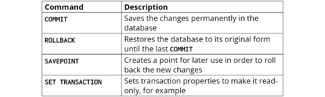
Figure 1.5: TCL commands

• Data Query Language (DQL): The final part of this section regarding the classification of commands is the DQL. This is used to fetch data from the database with the SELECT command. It's explained in detail in the following table:

Figure 1.6: DQL command

We'll look at these queries in detail in later chapters.

Creating Databases

An interesting point to note is that the create database command is not part of the regular SQL standard. However, it is supported by almost all database products today. The create database statement is straightforward. You just need to issue a database name along with the command, followed by a semicolon.

Let's start by creating a simple example database. We'll call it studentdemo. To create the studentdemo database with the default configuration, use the following command:

create database studentdemo;

To run this statement, click the Execute button (shaped like a lightning bolt):

Figure 1.7: Creating the studentdemo database

In the Action Output pane, the successful completion of a command will appear. You will also be able to see the newly created database in the Schemas tab of the Navigator pane.

Note

SQL is not case sensitive. This implies CREATE TABLE studentdemo; is the same as create table studentdemo;.

We cannot have multiple databases with the same name. If you try to run the query again, you'll get the following error:

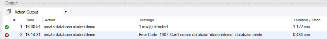
Figure 1.8: Error message displayed in the case of a database with the same name as another database

The Use of Semicolons

As you may have noticed, there's a semicolon, ;, at the end of the statement as an indication that that's the end of that statement. It depends on the database system you are using; some of them require a semicolon at the end of each statement and some don't, but you can still add it without worrying about the results.

Note

In general, it's good practice to use a semicolon at the end of a statement as it could play a significant role when we have multiple SQL statements or while writing a function or a trigger. This will be explained in more detail in the upcoming chapters. Throughout this book, we will use semicolons at the end of each statement.

Like every other programming language, SQL also has data types. Every piece of data that is entered into a database must comply with the data types and their formats. This implies that any data that you store is either a number, a character, or some other data type. Those are the basic data types. There are some special data types as well.

For instance, "00:43 on Monday, 1 April 2019" is a combination of letters, numbers, and punctuation. However, when we see something like this, we immediately start thinking of the day. A data type is the type of value that can be stored in a system. Some examples of data types are INTEGER, FLOATING POINT, CHARACTER, STRING, and combinations of these such as DATETIME.

Since there's a large amount of data types, most languages classify data types. Here, we will go through some of the most common ones. The idea here is to get you acquainted with the data types, not to give you a complete rundown of them as this would overwhelm you with hardly any significant returns. Moreover, once the concept is clear, you will be able to adapt to the rest of the data types with little effort.

In the interest of better data integrity and modeling, it is critical to select the right data type for the situation. It may seem trivial when the database is small, but with a larger database, it becomes difficult to manage. As a programmer, it is your responsibility to model your data in the right way.

In order to keep this simple, let's broadly classify the data types into five categories:

• Numeric data types: Numeric data types include everything that involves numbers, such as integers (small/big), floating- and fixed-point decimal numbers, and real numbers. Here are some of the most common ones:

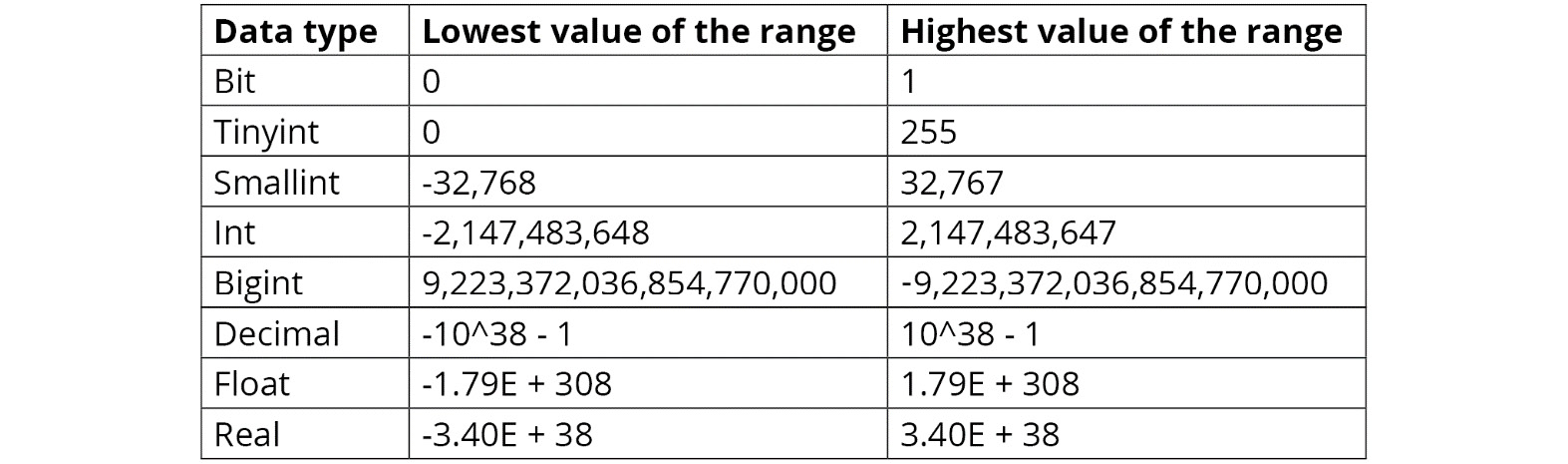
Figure 1.9: Numeric data types

• Fixed and varying length characters and text: Performance is key when selecting either fixed- or variable-length characters. When you know that a certain piece of data will be of a fixed number of characters, use the fixed width. For example, if you know that the employee code will always be of 4 characters, you can use CHAR. When you are unsure of the number of characters, use variable width. If a certain column holds only six characters, you are better off specifying it so that space used will be limited. By doing this, you will get better performance by not using up more resources than required. If you are unsure of the width, you don't want to be limited by the total width. Therefore, you should ideally use character types of varying lengths. An example of this can be a person's first name, where the length of the name is not fixed.

  Note

  You can use CHAR with varying lengths of characters (VARCHAR) as well. For instance, in a field that accepts up to six characters, you can enter data that is three characters long. However, you would be leaving the other three-character spaces unused, which will be right-padded, meaning that the remaining spaces will be reserved as actual spaces. When the data is retrieved, these trailing spaces will be trimmed. If you don't want them to be trimmed, you can set a flag in SQL that tells SQL to reserve the spaces and not trim them during retrieval. There are situations where you would need to do this using the TRIM string function, for example, to enhance data security.

  Unicode characters and string data types are different. They are prefixed with N, such as NCHAR, NVARCHAR, and NTEXT. Also, note that not all SQL implementations support Unicode data types.

  Note

  Unicode character data types consume twice the storage space compared to non-Unicode character data types.

  The other character-based data type is TEXT. This can store textual data up to a certain limit, which may vary with the system. For instance, MS SQL supports text up to 2 GB in size.

• Binary data types: Binary forms of data are also allowed in SQL. For instance, an IMAGE would be an object of binary form. Similarly, you have BINARY and VARBINARY data types.
• Miscellaneous data types: Miscellaneous data types include most of the now-popular data types, such as Binary Large Object (BLOB), Character Large Object (CLOB), XML, and JSON. We have included DATE, TIME, and DATETIME as well in this class.

  Character and binary large objects include types such as files. For instance, a film stored on Netflix is a binary large object. So would be an application package such as an EXE or an MSI, or other types of files such as PDFs.

  Note

  SQL Server 2016 supports JSON. JSON Unicode character representation uses NVARCHAR/NCHAR or ANSI VARCHAR/CHAR for non-Unicode strings.

  MySQL version 5.7.8 supports a native JSON data type.

• Proprietary types: In the real world, there is hardly a pure SQL implementation that is favored by enterprises. Different businesses have different requirements, and to cater to these requirements, SQL implementations have created their own data types. For instance, Microsoft SQL has MONEY as a data type.

  Not all data types are supported by all vendors. For instance, Oracle's implementation of SQL does not support DATETIME, while MySQL does not support CLOB. Therefore, the flavor of SQL is an important consideration when designing your database schema.

As we mentioned previously, this is not an exhaustive list of all data types. Your flavor of SQL will have its own supporting set of data types. Read the documentation that comes with the product kit to find out what it supports—as a programmer or a SQL administrator, it is you who decides what is necessary. This book will empower you to do that.

The size limits illustrated in Figure 1.9 are only indicative. Just as different flavors of databases may have different data types, they may have different limits as well. The documentation that accompanies the product you plan to use will have this information.

After creating the database, we want to create a table The create table statement is part of the SQL standard. The create table statement allows you to configure your table, your columns, and all your relations and constraints. Along with the create table command, you're going to pass the table name and a list of column definitions. At the minimum for every column, you must provide the column name and the data type the column will hold.

Let's say you want to add a table called Student to the previously created database, studentdemo, and you want this table to contain the following details:

• Student name: The student's full name.
• Student ID: A value to identify each student uniquely.
• Grade: Each student is graded as A, B, or C based on their performance.
• Age: The age of the student.
• Course: The course they are enrolled on.

To achieve this, we need to complete a two-step process:

1. To set the current database as studentdemo, enter the following code in the new query tab:
   

   Figure 1.10: Switching from the default database to our database

   You can open a new query tab, by clicking File | New Query Tab.

2. Create a table Student within studentdemo with the following columns:

   create table Student
   (
       StudentID      CHAR (4), 
       StudentName VARCHAR (30), 
       grade       CHAR(1), 
       age         INT, 
       course      VARCHAR(50),
       PRIMARY KEY (StudentID)
   );

The preceding code creates a Student table with the following columns:

• StudentID will contain four character values. 'S001', 'ssss', and 'SSSS' are all valid inputs and can be stored in the StudentID field.
• grade will just contain a single character. 'A', 'F', 'h', '1', and 'z' are all valid inputs.
• StudentName will contain variable-length values, which can be 30 characters in size at most. 'John', 'Parker', 'Anna', 'Cleopatra', and 'Smith' are all valid inputs.
• course will also contain variable-length values, which can be 50 characters in size at most.
• age will be an integer value. 1, 34, 98, 345 are all valid values.

StudentID is defined as the primary key. This implies that all the values in the StudentID field will be unique, and no value can be null. You can uniquely identify any record in the Student table using StudentID. We will learn about primary keys in detail in Chapter 3, Normalization.

Note

NULL is used to represent missing values.

Notice that we have provided the PRIMARY KEY constraint for StudentID because we require this to be unique.

Once your table has been created successfully, you will see it in the Schemas tab of the Navigator pane:

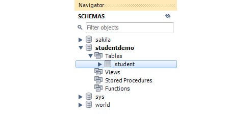
Figure 1.11: The Schemas tab in the Navigator pane

Exercise 1.01: Building the PACKT_ONLINE_SHOP Database

In this exercise, we're going to start building the database for a Packt Online Shop—a store that sells a variety of items to customers. We will be using the MySQL Community Server in this book. The Packt Online Shop has been working on spreadsheets so far, but as they plan to scale up, they realize that this is not a feasible option, and so they wish to move toward data management through SQL. The first step in this process will be to create a database named PACKT_ONLINE_SHOP with a table for storing their customer details. Perform the following steps to complete this exercise:

1. Create a database using the create statement:

   create database PACKT_ONLINE_SHOP;

2. Switch to this database:

   use PACKT_ONLINE_SHOP;

3. Create the Customers table:

   create table Customers
   (
       FirstName varchar(50) ,
       MiddleName varchar(50) ,
       LastName varchar(50) ,
       HomeAddress varchar(250) ,
       Email varchar(200) ,
       Phone varchar(50) ,
       Notes varchar(250)
   );

   Note

   Similar to varchar, nvarchar is a variable-length data type; however, in nvarchar, the data is stored in Unicode, not in ASCII. Therefore, columns defined with nvarchar can contain values in other languages as well. nvarchar requires 2 bytes per character, whereas varchar uses 1 byte.

4. Execute the statement by clicking the Execute button:
   

   Figure 1.12: Creating the Customers table

5. Review the table by right-clicking the table in the Schemas tab and clicking Select Rows - Limit 1000 in the contextual menu:

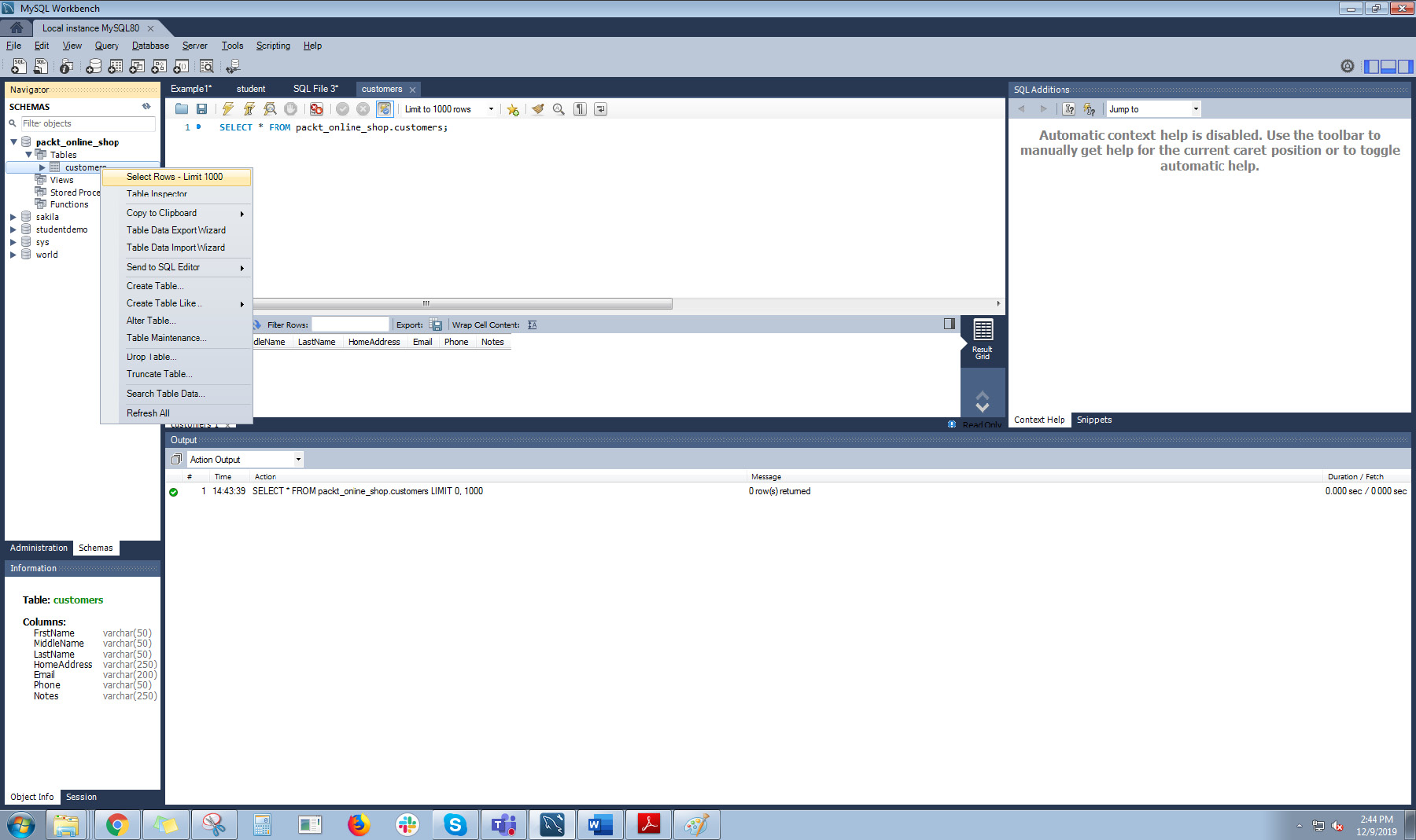
Figure 1.13: Column headers displayed through the SELECT query

This runs a simple Select query. You will learn about the Select statement in Chapter 4, The SELECT Statement. The top 1,000 rows are displayed. Since we have not inserted values into the table yet, we are only able to view the column headers in Result Grid.

Note

If you are working on Microsoft SQL Server, you can do this by right-clicking the table in the Object Explorer window and then selecting Select Top 1000 Rows.

In the next section, we will look at inserting values into tables.

Once the table has been created, the next logical step is to insert values into the table. To do this, SQL provides the INSERT statement. Let's try adding a row of data to the Student table of the studentdemo database that we created previously.

Here is the SQL statement to achieve this. First, switch to the studentdemo database and enter the following query:

USE studentdemo;
INSERT INTO Student (StudentID, StudentName, grade, age, course) VALUES ('S001', 'Prashanth Jayaram', 'A', 36, 'Computer Science');

If you check the contents of the database after running this query, you should see something like this:

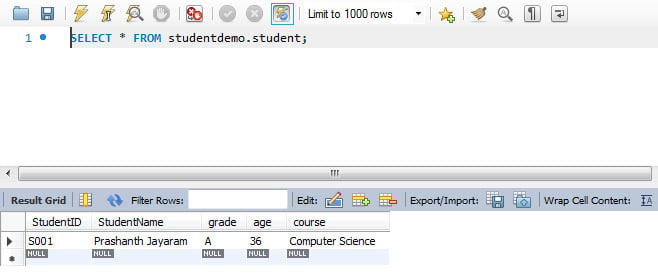
Figure 1.14: Values inserted into the database

Note

To see the contents of this database, follow the process you used in the earlier exercises. Right-click the table and choose Select Rows - Limit 1000.

Adding single rows like this in multiple queries will be time-consuming. We can add multiple rows by writing a query like the following one:

INSERT INTO Student (StudentID, StudentName, grade, age, course) VALUES ('S002', 'Frank Solomon', 'B', 35, 'Physics'), ('S003', 'Rachana Karia', 'B', 36, 'Electronics'), ('S004', 'Ambika Prashanth', 'C', 35, 'Mathematics');

The preceding query looks like this on the Query tab.

Figure 1.15: Adding multiple rows in an INSERT query

When you run the query, all three rows will be added with a single query:

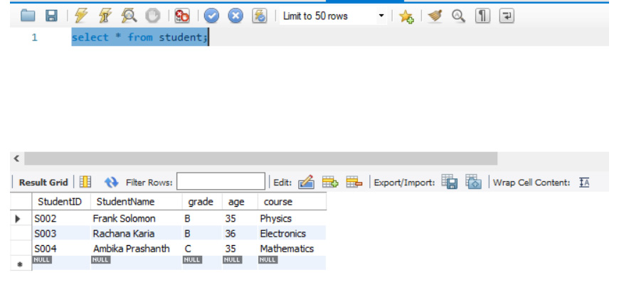
Figure 1.16: Output of multiple row insertion

Exercise 1.02: Inserting Values into the Customers Table of the PACKT_ONLINE_SHOP Database

Now that we have the Customers table ready, let's insert values into the table using a single query. We have the data from an already existing Excel spreadsheet. We will be using that data to write our query. Here is what the Excel file looks like:

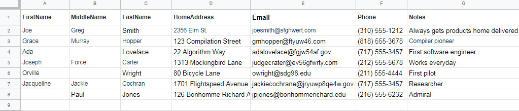
Figure 1.17: Source data in an Excel spreadsheet

Note

You can find the csv format of the file here: https://packt.live/369ytTu.

To move this data into the database, we will need to perform the following steps:

1. Switch to the PACKT_ONLINE_SHOP database:

   use PACKT_ONLINE_SHOP;

2. Insert the values based on the Excel spreadsheet provided wherever we have blank data. We will use NULL to do this:

   INSERT INTO Customers (FirstName, MiddleName, LastName, HomeAddress, Email, Phone, Notes)
   VALUES('Joe', 'Greg', 'Smith', '2356 Elm St.', 'joesmith@sfghwert.com', '(310) 555-1212', 'Always gets products home delivered'),
   ('Grace', 'Murray', 'Hopper', '123 Compilation Street', 'gmhopper@ftyuw46.com', '(818) 555-3678', 'Compiler pioneer'),
   ('Ada', NULL, 'Lovelace', '22 Algorithm Way', 'adalovelace@fgjw54af.gov', '(717) 555-3457', 'First software engineer'),
   ('Joseph', 'Force', 'Crater', '1313 Mockingbird Lane', 'judgecrater@ev56gfwrty.com', '(212) 555-5678', 'Works everyday'),
   ('Jacqueline', 'Jackie', 'Cochran', '1701 Flightspeed Avenue', 'jackiecochrane@jryuwp8qe4w.gov', '(717) 555-3457', 'Researcher'),
   (NULL, 'Paul', 'Jones', '126 Bonhomme Richard Ave.', 'jpjones@bonhommerichard.edu', '(216) 555-6232', 'Admiral');

3. When you execute the query and check the contents of the Customers table, you should see the following output.
   

Figure 1.18: The Customers table after inserting the values from the excel sheet

With this, you have successfully populated the Customers table.

Activity 1.01: Inserting Values into the Products Table in the PACKT_ONLINE_SHOP Database

Now that we've migrated the customer's data into the database, the next step is to migrate the product data from the Excel spreadsheet to the database. The data to be entered into the database can be found at https://packt.live/2ZnJiyZ.

Here is a screenshot of the Excel spreadsheet:

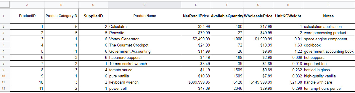
Figure 1.19: Source data in an Excel spreadsheet

1. Create a table called Products in the Packt_Online_Shop database.
2. Create the columns as present in the Excel sheet.
3. Use the INSERT statement to input the required data into the table.

   Note

   The solution for this activity can be found via this link.

In this chapter, we had a look at the different types of data and how data is stored in relational databases. We also had a brief look at the different commands available in SQL. We specifically focused on creating databases and tables within the databases, as well as how we can easily insert values into tables.

In the next chapter, we will look at how we can modify the data, the properties of tables, and databases, and build complex tables.