Talk is cheap. Show me the code.

—Linus Torvalds

There is not just one way to code, and there is not only one programming language in which to do it. A recent survey by the analyst firm RedMonk listed the top one hundred languages in widespread use in 2021. [PLR]

Nevertheless, there are common ideas about processing and computing with information across programming languages, even if their expressions and implementations vary. In this chapter, I introduce those ideas and data structures. I don’t focus on how we write everything in any particular language but instead discuss the concepts. I do include some examples from other languages to show you the variation of expression.

If you think of all the digital data and information stored in the cloud, on the web, on your phone, on your laptop, in hard and solid-state drives, and in every computer transaction, consideration comes down to just two things: 0 and 1.

These are bits, and with bits we can represent everything else in what we call “classical computers.” These systems date back to ideas from the 1940s. There is an additional concept for quantum computers, that of a qubit or “quantum bit.” The qubit extends the bit and is manipulated in quantum circuits and gates. Before we get to qubits, however, let’s consider the bit more closely.

First, we can interpret 0 as false and 1 as true. Thinking in terms of data, what would you say if I asked you the question, “Do you like Punk Rock?” We can store your response as 0 or 1 and then use it in further processing, such as making music recommendations to you. When we talk about true and false, we call them Booleans instead of bits.

Second, we can treat 0 and 1 as the numbers 0 and 1. While that’s nice, if the maximum number we can talk about is 1, we can’t do any significant computation. So, we string together more bits to make larger numbers. The binary numbers 00, 01, 10, and 11 are the same as 0, 1, 2, and 3 when we use a decimal representation. Using even more bits, we represent 72 decimal as 1001000 binary and 83,694 decimal as 10100011011101110 binary.

decimal: 72 = 7 × 10¹ + 2 × 10⁰
binary: 1001000 = 1 × 2⁶ + 0 × 2⁵ + 0 × 2⁴ + 1 × 2³ + 0 × 2² + 0 × 2¹ + 0 × 2⁰

With slightly more sophisticated representations, we can store and use negative numbers. We can also create numbers with decimal points, also known as floating-point numbers. [FPA] We use floating-point numbers to represent or approximate real numbers. Whatever programming language we use, we must have a convenient way to work with all these kinds of numbers.

When we think of information more generally, we don’t just consider numbers. There are words, sentences, names, and other textual data. In the same way that we can encode numbers using bits, we create characters for text. Using the Extended ASCII standard, for example, we can create my nickname, “Bob”: [EAS]

01000010 → B
01101111 → o
01100010 → b

Each run of zeros and ones on the left-hand side has 8 bits. This is a byte. One thousand (10³) bytes is a kilobyte, one million (10⁶) is a megabyte, and one billion (10⁹) is a gigabyte.

If we limit ourselves to a byte to represent characters, we can only represent 256 = 2⁸ of them. If you look at the symbols on a keyboard, then imagine other alphabets, letters with accents and umlauts and other marks, mathematical symbols, and emojis, you will count well more than 256. In programming, we use the Unicode standard to represent many sets of characters and ways of encoding them using multiple bytes. [UNI]

When we put characters next to each other, we get strings. Thus "abcd" is a string of length four. I’ve used the double quotes to delimit the beginning and end of the string. They are not part of the string itself. Some languages treat characters as special objects unto themselves, while others consider them to be strings of length one.

This is a good start for our programming needs: we have bits and Booleans, numbers, characters, and strings of multiple characters to form text. Now we need to do something with these kinds of data.

An expression is a written combination of data with operations to perform on that data. That sounds quite formal, so imagine a mathematical formula like:

15 × 6² + 3 × 6 – 4 .

This expression contains six pieces of data: 15, 6, 2, 3, 6, and 4. There are five operations: multiplication, exponentiation, addition, multiplication, and subtraction. If I rewrite this using symbols often used in programming languages, it is:

15 * 6**2 + 3 * 6 - 4

See that repeated 6? Suppose I want to consider different numbers in its place. I can write the formula:

15 × x² + 3 × x – 4

and the corresponding code expression:

15 * x**2 + 3 * x - 4

If I give x the value 6, I get the original expression. If I give it the value 11, I calculate:

15 * 11**2 + 3 * 11 - 4

We call x a variable and the process of giving it a value assignment. The expression

x = 11

means “assign the value 11 to x and wherever you see x, substitute in 11.” There is nothing special about x. I could have used y or something descriptive like kilograms.

An expression can contain multiple variables.

The way we write data, operations, variables, names, and words together with the rules for combining them is called a programming language’s syntax. The syntax must be unambiguous and allow you to express your intentions elegantly. In this chapter, we do not focus on syntax but more on the ideas and the meaning, the semantics, of what programming languages can do. In Chapter 2, Working with Expressions, we begin to explore the syntax and features of Python.

We’re not limited to arithmetic in programming. Given two numbers x and y, if I saw maximum(x, y), I would expect it to return the larger value. Here “maximum” is the name of a function. We can write our own or use functions created, tested, optimized, and stored in libraries by others.

The notion of “expression” includes functions and all that goes into writing and using them. The syntax of their definition varies significantly among programming languages, unlike simple arithmetic expressions. In words, I can say

The function maximum(x, y) returns x
if it is larger than y. Otherwise, it returns y.

Let’s consider this informal definition.

• It has a descriptive name: maximum.
• There are two variables within parentheses: x and y. These are the parameters of the function.
• A function may have zero, one, two, or more parameters. To remain readable, it shouldn’t have too many.
• When we employ the function as in maximum(3, -2) to get the larger value, we call the function maximum on the arguments 3 and -2.
• To repeat: x and y are parameters, and 3 and -2 are arguments. However, it’s not unusual for coders to call them all arguments.
• The body of the function is what does the work. The statement involving if-then-otherwise is called a conditional. Though “if” is often used in programming languages, the “then” and “otherwise” may be implicit in the syntax used to write the expression. “else” or a variation may be present instead of “otherwise.”
• The test “x larger than y” is the inequality x > y. This returns a Boolean true or false. Some languages use “predicate” to refer to an expression that returns a Boolean.
• maximum returns a value that you can use in further computation. Coders create some functions for their actions, like updating a database. They might not return anything.

For comparison, this is one way of writing maximum in the C programming language:

int maximum(int x, int y) {
    if (x > y) {
        return x;
    }
    return y;
}

This is a Python version with a similar definition:

def maximum(x, y):
    if x > y:
        return x
    return y

There are several variations within each language for accomplishing the same result. Since they look so similar in different languages, you should always ask, “Am I doing this the best way in this programming language?”. If not, why are you using this language instead of another?

Expressions can take up several lines, particularly function definitions. C uses braces “{ }” to group parts together, while Python uses indentation.

While many books are now digital and available online, physical libraries are often still present in towns and cities. You can use a library to avoid doing something yourself, namely, buying a book. You can borrow it and read it. If it is a cookbook, you can use the recipes to make food.

A similar idea exists for programming languages and their environments. I can package together reusable data and functions, and then place them in a library. Via download or other sharing, coders can use my library to save themselves time. For example, if I built a library for math, it could contain functions like maximum, minimum, absolute_value, and is_prime. It could also include approximations to special values like π.

Once you have access to a library by installing it on your system, you need to tell your programming environment that you want to take advantage of it. Languages use different terminology for what they call the contents of libraries and how to make them available.

• Python imports modules and packages.
• Go imports packages.
• JavaScript imports bindings from modules.
• Ruby requires gems.
• C and C++ include source header files that correspond to compiled libraries for runtime.

In languages like Python and Java, you can import specific constructs from a package, such as a class, or everything in it. With all these examples, the intent is to allow your environment to have a rich and expandable set of pre-built features that you can use within your code. Some libraries come with the core environment. You can also optionally install third-party libraries. Part III of this book looks at a broad range of frequently used Python libraries.

What happens if you import two libraries and they each have a function with the same name? If this happens, we have a naming collision and ambiguity. The solution to avoid this is to embellish the function’s name with something else, such as the library’s name. That way, you can explicitly say, “use this function from here and that other function from over there.” For example, math.sin in Python means “use the sin function from the math module.” This is the concept of a namespace.

Returning to the book analogy we started when discussing libraries, imagine that you own the seven volumes in the Chronicles of Narnia series by C. S. Lewis.

• The Lion, the Witch and the Wardrobe
• Prince Caspian: The Return to Narnia
• The Voyage of the Dawn Treader
• The Silver Chair
• The Horse and His Boy
• The Magician’s Nephew
• The Last Battle

The order I listed them is the order in which Lewis published the volumes from 1950 through 1956. In the list, the first book is the first published, the second is the second published, and so on. Had someone been maintaining the list in the 1950s, they would have appended a new title when Lewis released a new book in the series.

A programming language needs a structure like this so that you can store and insert objects as above. It shouldn’t surprise you that this is called a list. A list is a collection of objects where the order matters.

If we think of physical books, you can see that lists can contain duplicates. I might have two paperback copies of The Lion, the Witch and the Wardrobe, and three of The Horse and His Boy. The list order might be based on when I obtained the books.

Another simple kind of collection is a set. Sets contain no duplicates, and the order is not specified nor guaranteed. We can do the usual mathematical unions and intersections on our sets. If I try to insert an object into a set, it becomes part of the set only if it is not already present.

The third basic form of collection is called a dictionary or hash table. In a dictionary, we connect a key with a value. In our example, the key could be the title and the value might be the book itself. You see this for eBooks on a tablet or phone. You locate a title within your library, press the text on the screen with your finger, and the app displays the text of the book for you to read. A key must be unique: there can be one and only one key with a given name.

Authors of computer science textbooks typically include collections among data structures. With these three collections mentioned above, you can do a surprising amount of coding. Sometimes you need specialized functionality such as an ordered list that contains no duplicates. Most programming libraries give you access to a broad range of such structures and allow you to create your own.

C. S. Lewis wrote many other books and novels. Another dictionary we could create might use decades like “1930s”, “1940s”, “1950s”, and “1960s” as the keys. The values could be the list of titles in chronological order published within each ten-year span.

Collections can be parts of other collections. For example, I can represent a table of company earnings as a list of lists of numbers and strings. However, some languages require the contained objects all to be of the same type. For example, maybe a list needs to be all integers or all strings. Other languages, including Python, allow you to store different kinds of objects.

An object which we can change is called mutable. The list of books is mutable while an author is writing and publishing. Once the author passes away, we might lock the collection and declare it immutable. No one can make any further changes. For dictionaries, the keys usually need to be immutable and are frequently strings of text or numbers.

When you write code, you create instructions for a computer that state what steps the computer must take to accomplish some task. In that sense, you are specifying a recipe. Depending on some conditions, like if a bank balance is positive or a car’s speed exceeds a stated limit, the sequence of steps may vary. We call how your code moves from one step to another its flow.

Let’s make some bread to show where a basic recipe has points where we should make choices.

Ingredients

• 1 ½ tablespoons sugar
• ¾ cup warm water (slightly warmer than body temperature)
• 2 ¼ teaspoons active dry yeast (1 package)
• 1 teaspoon salt
• ½ cup milk
• 1 tablespoon unsalted butter
• 2 cups all-purpose flour

Straight-through recipe

1. Combine sugar, water, and yeast in a large bowl. Let sit for 10 minutes.
2. Mix in the salt, milk, butter, and flour. Stir with a spatula or wooden spoon for 5 minutes.
3. Turn out the dough onto a floured counter or cutting board. Knead for 10 minutes.
4. Butter a large bowl, place the dough in it, turn the dough over to cover with butter.
5. Cover the bowl and let it sit in a warm place for 1 hour.
6. Punch down the dough and knead for 5 minutes. Place in a buttered baking pan for 30 minutes.
7. Bake in a pre-heated 375° F (190° C, gas mark 5) oven for 45 minutes.
8. Turn out the loaf of bread and let it cool.

Problems

I call that a “straight-through” recipe because you do one step after another from the beginning to the end. The flow proceeds in a straight line with no detours. However, the recipe is too simple because it does not include conditions that must be met before moving to later steps.

• In step 1, your bread will not rise if the yeast is dead. We must ensure that the mixture is active and foamy.
• In step 2, we need to add more flour in little portions until the stirred dough pulls away from the bowl.
• In step 3, if the dough gets too sticky, we need to add even more flour.
• In step 5, an hour is only an estimate for the time it will take for the dough to double in size. It may take more or less time.
• In step 6, we want the dough to double in size in the loaf pan.
• In step 7, 45 minutes is an estimate for the baking time for the top of the bread to turn golden brown.

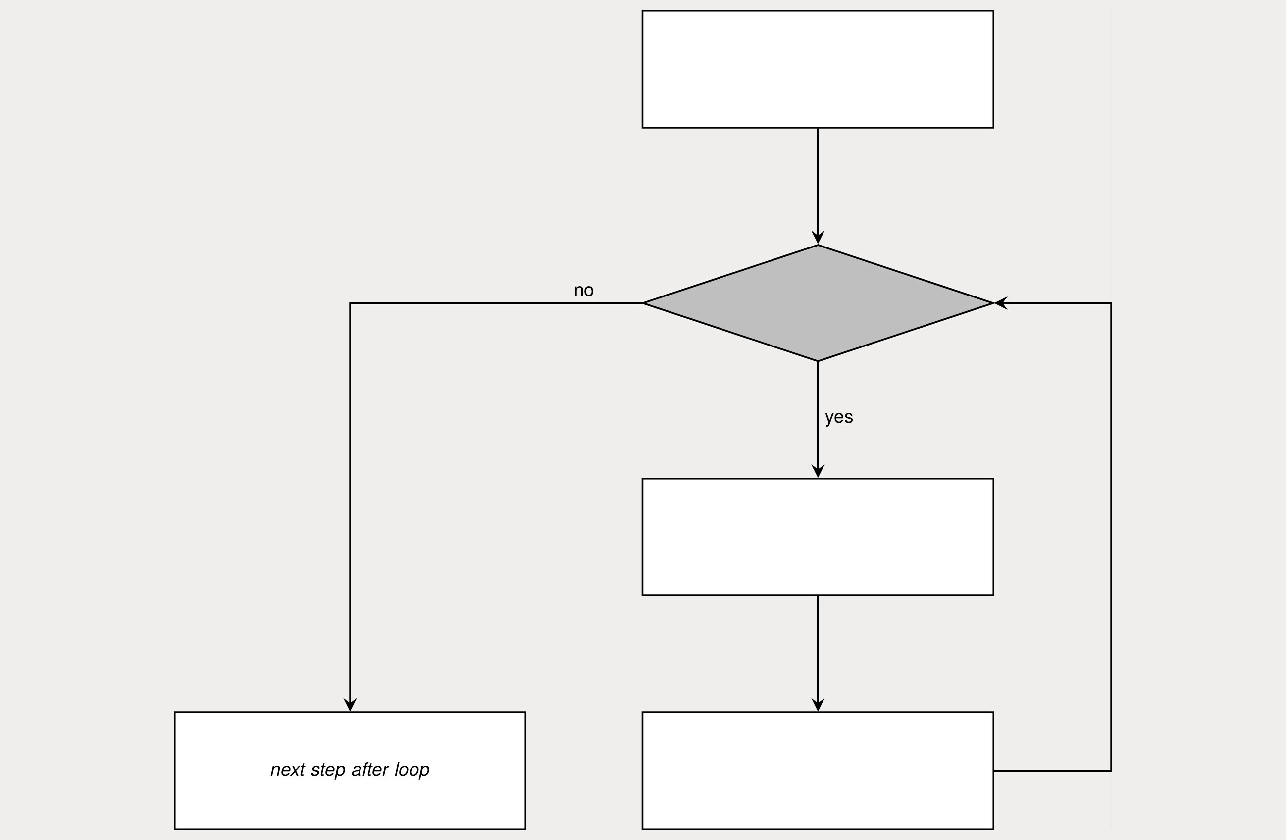
Conditional recipe

1. Combine sugar, water, and yeast in a large bowl. Let sit for 10 minutes. If the mixture is foamy, then continue to the next step. Otherwise, discard the mixture, and combine sugar, water, and fresh yeast in a large bowl. Let sit for 10 minutes.
2. Mix in the salt, milk, butter, and flour. Stir with a spatula or wooden spoon for 5 minutes. If the mixture does not pull aside from the sides of the bowl, then add 1 tablespoon of flour and stir for 1 more minute. Otherwise, continue to the next step.
3. Turn out the dough onto a floured counter or cutting board. Knead for 10 minutes. If the mixture is sticky, then add 1 tablespoon of flour and stir for 1 more minute. Otherwise, continue to the next step.
4. Butter a large bowl, place the dough in it, turn the dough over to cover with butter.
5. Cover the bowl and let it sit in a warm place for 1 hour. If the dough has not doubled in size, then let it sit covered in the bowl for 15 more minutes. Otherwise, continue to the next step.
6. Punch down the dough and knead for 5 minutes. Place in a buttered baking pan for 30 minutes. If the dough has not doubled in size, then let it sit covered in the baking pan for 15 more minutes. Otherwise, continue to the next step.
7. Bake in a pre-heated 375° F (190° C, gas mark 5) oven for 45 minutes. If the top of the bread is not golden brown, then bake for 5 more minutes. Otherwise, continue to the next step.
8. Turn out the loaf of bread and let cool.

Figure 1.2 is a flowchart, and it shows what is happening in the first step. The rectangles are things to do, and the diamond is a decision to be made that includes a condition.

You may find it useful to use such a chart to map out the flow of your code.

These instructions are better. We test several conditions to determine the next course of action. We still are not checking whether a condition is met after repeating a step multiple times.

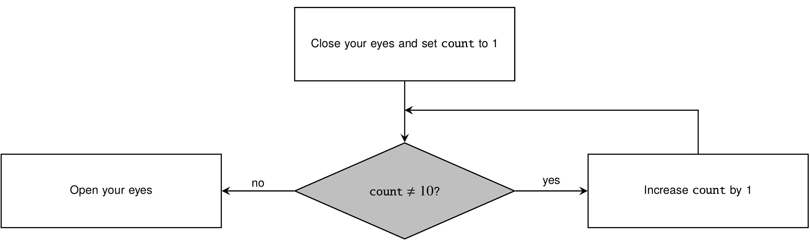
If I ask you to close your eyes, count to 10, then open them, the steps look like this:

1. Close your eyes
2. Set count to 1
3. While count is not equal 10, increment count by 1
4. Open your eyes

Steps 2 and 3 together constitute a loop. In this loop, we repeatedly do something while a condition is met. We do not move to step 4 from step 3 while the test returns true.

Compare the simplicity of Figure 1.3 to

1. Close your eyes
2. Set count to 1
3. Increment count to 2
4. Increment count to 3
5. …
6. Increment count to 10
7. Open your eyes

If that doesn’t convince you, imagine if I asked you to count to 200. Here is how we do it in C++:

int n = 1;

while( n < 201 ) {
    n++;
}

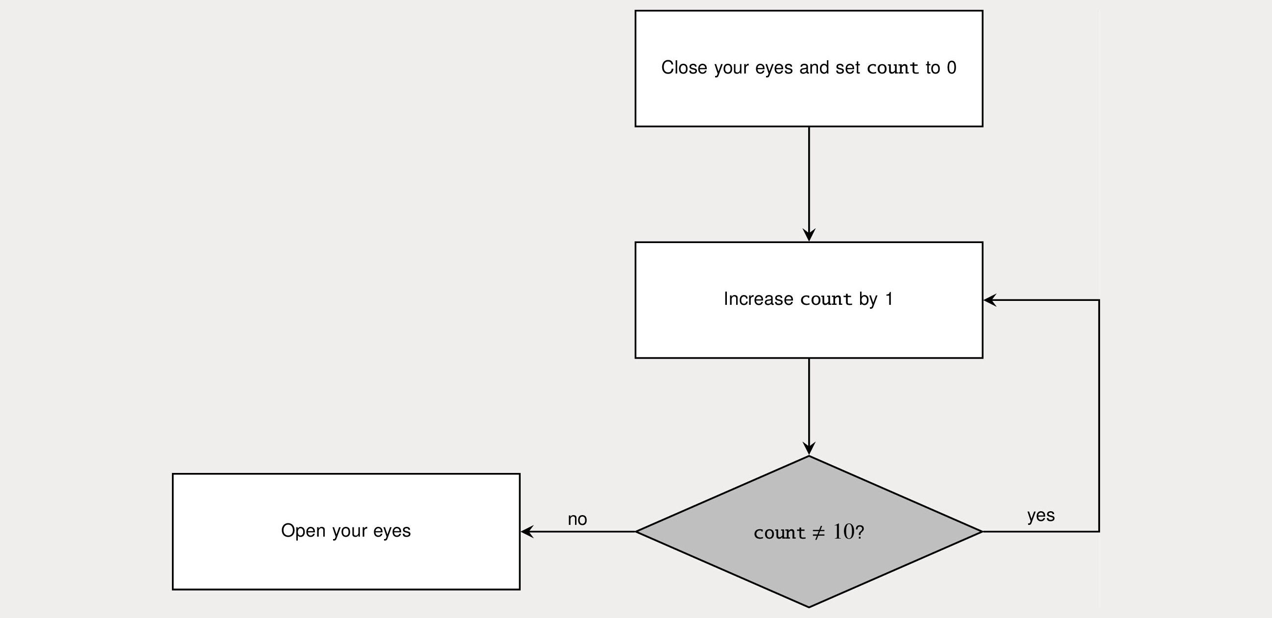
That loop was a while-loop, but this is an until-loop:

1. Close your eyes
2. Set count to 1
3. Increment count by 1 until count equals 10
4. Open your eyes

Many languages do not have until-loops, but VBA does:

n = 1
Do Until n>200
    n = n + 1
Loop

We saw earlier that the code within a function’s definition is its body. The repeated code in a loop is also called its body.

Exercise 1.7

What is different between while-loops and until-loops regarding when you test the condition? Compare this until-loop flowchart with the previous while-loop example.

Our next example is a for-loop, so named because of the keyword that many programming languages use. A for-loop is very useful when you want to repeat something a specified number of times. This example uses the Go language:

sum := 0
for n := 1; n <= 50; n++ {
    sum += n
}

It adds all the numbers between 1 and 50, storing the result in sum. Here, := is an assignment, n++ means “replace the value of n by its previous value plus 1,” and sum += n means “replace the value of sum by its previous value plus the value of n.”

There are four parts to this particular syntax for the for-loop:

• the initialization: n := 1
• the condition: n <= 50
• the post-body processing code: n++
• the body: sum += n

The sequence is: do the initialization once; test the condition and, if true, execute the body; execute the post-body code; test the condition again and repeat. If the condition is ever false, the loop stops, and we move to whatever code follows the loop.

Exercise 1.9

Draw a flowchart of a for-loop, including the initialization, condition, post-body processing code, and the body. Use the template in Figure 1.5.

In many science fiction stories, novels, movies, and television series, characters use “teleportation” to move people and objects from one place to another. For example, the protagonist could teleport from Toronto to Tokyo instantly, without going through the time-consuming hassle of air flight.

It is also used in such plots to allow characters to escape from dangerous and unexpected conditions. Perhaps a monster might have the team cornered in the back of a cave, and there is no way to fight their way to safety. A hurried call by the leader on a communications device might demand “get us out of here!” or “beam us up now!” The STAR TREK^® series and movies often featured the latter exclamation.

So, characters use teleportation for regular transportation, but also for exceptional situations that are usually life-threatening. Many programming languages also have the concept and mechanism of exceptions.

In a loop or a well-written function, you can see how your code’s execution moves from one step to another. With an exception, you say, “try this, and if it doesn’t work out, come back here.” Or, you might be thinking, “I’m going about my business, but something may happen infrequently, and I need to handle it if it does.” The place in your code where you handle the exception is called its catch point.

Suppose you want to delete a file. You have its name, and you call a function to remove the file. The only problem is that the file does not exist. How do you handle this? One way is to use a condition: if the file exists, then delete it. Another way is to use an exception: try to delete the file, and if something goes wrong (for example, it doesn’t exist), raise an exception, and go back and decide what you should do about it.

Another good example of why you might raise an exception is division by zero. Something is seriously wrong in your code if it tries to do this, and the solution may not be obvious to you. Using an exception can help you find processing or code design errors.

An exception usually includes information that explains why it was raised. Perhaps we could not delete the file because it wasn’t present. Alternatively, maybe we didn’t have permission to delete it. When we catch the exception, we can see what happened and proceed accordingly.

An exception can be raised and caught within a single function. Or, it might originate hundreds of steps away from the catch point. Functions often call other functions, which call yet other functions. The exception could be raised from one of these deeply nested function executions.

The philosophy and accepted conventions for using exceptions vary from programming language to programming language. Like several topics in software development, exceptions can be the focus of fervor and heated debate.

Consider this one-sentence paragraph with some text formatted in bold and italics:

Some words are bold, some are italic, and some are both.

How could you represent this as data in a word processor, spreadsheet, or presentation application?

Let’s begin with the text itself for the paragraph. Maybe we just use a string.

"Some words are bold, some are italic, and some are both."

The words are there, but we lost the formatting. Let’s break the sentence into a list of the formatted and unformatted parts. I use square brackets “[ ]” around the list and commas to separate the parts.

[ "Some words are ",
  "bold",
  ",some are ",
  "italic",
  ", and some are ",
  "both",
  "." ]

Now we can focus on how to embellish each part with formatting. There are four options:

1. the text has no formatting,
2. the text is only bold,
3. the text is only italic, and
4. the text is both bold and italic.

Each part needs three pieces of information: the string holding the text, a Boolean indicating whether it is bold, and another Boolean indicating whether it is italic.

[ {text: "Some words are ", bold: false, italic: false},
  {text: "bold", bold: true, italic: false},
  {text: ",some are ", bold: false, italic: false},
  {text: "italic", bold: false, italic: true},
  {text: ", and some are ", bold: false, italic: false},
  {text: "both", bold: true, italic: true},
  {text: ".", bold: false, italic: false} ]

The object that I’ve shown inside braces “{ }” is a record. It has named members that I can access independently.

Languages often use a period “.” to access the value for a member. If I assign the first record in the list to the variable “part_1,” you might see something like part_1.text or part_1.italic in the code. The values are “Some words are ” and false.

In C, a record is called a struct, and most languages have some way of representing records. The syntax I used in the example is not Python.

While records allow us to create objects with constituent parts, they are not much better than lists that contain items of different types, such as integers and strings. We need to raise the level of abstraction and make new kinds of objects that have functions that work just on them. We also want to hide the representation and workings of these new compound objects. That way, we can alter and improve them without breaking dependent code and applications.

Let’s return to cooking. I recently ran out of bay leaves in our kitchen. Bay leaves are used to flavor many foods, most notably soups, stews, and other braised meat dishes. Okay, I thought, I’ll just order some bay leaves online. I found four varieties:

• Turkish or Mediterranean bay leaves, from the Bay Laurel tree,
• Indian bay leaves,
• California bay leaves, and
• Caribbean bay leaves.

I eventually discovered that what I wanted was Turkish bay leaves. I ordered six ounces. When they arrived, I realized that I had enough to last the rest of my life.

Let’s get back to the varieties. While numbers and strings are built into most programming languages, bay leaves most certainly are not. Nevertheless, I want to create a structure to represent bay leaves in a first-class way. Perhaps I’m building up a collection of ingredient objects to use in digital recipes.

Before we consider bay leaves in particular, let’s think about leaves in general. Without worrying about syntax, we define a class called Leaf. It has two properties: is_edible and latin_name.

Once I create a Leaf object, you can ask if it is edible and what its Latin name is. Depending on the programming language, you can either examine the property directly or use a function on an object of class Leaf to get the information.

A function that operates on an object of a class is called a method.

For most users of the class, it is best to call a method to get object information. I do not want to publish to the world how I store and manipulate that data for objects. If I do this, I, as the class designer, am free to change the internal workings. For example, maybe I initially store the Latin names as strings, but I later decide to use a database. If a user of Leaf assumed I always had a string present, their code would break when I changed to using the database.

This hiding of the internal workings of classes is called encapsulation.

Now we define a class called BayLeaf, and we make it a child class of Leaf. Every BayLeaf object is also a Leaf. All the methods and properties of Leaf are also those of BayLeaf. Leaf is the parent class of BayLeaf.

Moreover, I can redefine the methods in BayLeaf that I inherit from Leaf to make them correct or more specific. For example, by default, I might define Leaf so that an object of that type always returns false when asked if it is edible. I override that method in BayLeaf so that it returns true.

I can add new properties and methods to child classes as well. Perhaps I need methods that list culinary uses, taste, and calories per serving. These are appropriate to objects of BayLeaf because they are edible, but not to all objects in class Leaf. Every object that is a bay leaf should be able to provide this information.

Continuing in this way, I define four child classes of BayLeaf: TurkishBayLeaf, IndianBayLeaf, CaliforniaBayLeaf, and CaribbeanBayLeaf. These can provide specific information about taste, say, and this can vary among the varieties.

In many languages, a class can have at most one parent. In some, multiple inheritance is allowed, but the languages provide special rules for properties and methods. That’s especially important when there are name collisions; two methods from different parents may have the same name but different behavior. Which method is called? For an analogy, consider the rules of genetics that determine the eye color of a child.

If we define the Herb class, then we can draw this class hierarchy. The arrows point from the class parents to their children.

In this example involving bay leaves, the methods returned information. If I create a class for polynomials that all use the same variable, then I would likely define methods for addition, subtraction, negation, multiplication, quotient and remainder, degree, leading coefficient, and so forth.

In this section, I discussed what we call object-oriented programming (OOP) as it is implemented in languages like Python, C++, Java, and Swift. The terms superclass and subclass often replace parent class and child class, respectively. Once you are familiar with Python’s style of OOP, I encourage you to look at alternative approaches, such as how JavaScript does it.

In the first section of this chapter, we looked at data. Starting with the bits 0 and 1, we built integers, and I indicated that we could also represent floating-point numbers. Let’s switch from the arithmetic and algebra of numbers to geometry.

A single point is 0-dimensional. Two points are just two 0-dimensional objects. Let’s label these points 0 and 1. When we draw an infinite line through the two points and consider all the points on the line, we get a 1-dimensional object. We can represent each such point as (x), or just x, where x is a real number. If we have another line drawn vertically and perpendicular to the first, we get a plane. A plane is 2-dimensional, and we can represent every point in it with coordinates (x, y). The point (0, 0) is the origin.

This is the Cartesian geometry you learned in school. As we move from zero dimensions to two in Figure 1.7, we can represent more information. In an imprecise sense, we have more room in which to work. We can even link together the geometry of the plane with complex numbers, which extend the real numbers. We see those in section 5.5.

Now I want you to think about taking the standard 2-dimensional plane and wrapping it completely around a sphere. If that request strikes you as bizarre, consider this: start with a sphere and balance the plane on top. Make the origin of the plane sit right on the north pole of the sphere. Now start uniformly bending the plane down over the sphere, compressing it together as you move out from the origin.

Carry this to its completion, and the “infinity” ∞ of the plane sits at the south pole. In mathematical terms, this is a stereographic projection of the plane onto the sphere.

That was mind-warping as well as plane-warping! The sphere sits in three dimensions, but we can think about its surface as two-dimensional.

With that geometric discussion as the warm-up, I am now ready to introduce the qubit, which is short for “quantum bit.” While a bit can only be 0 or 1, a qubit can exist in more states. Qubits are surprising, fascinating, and powerful. They follow strange rules which may not initially seem natural to you. According to physics, these rules may be how nature itself works at the level of electrons and photons.

A qubit starts in an initial state. We use the notation |0⟩ and |1⟩ when we are talking about a qubit instead of the 0 and 1 for a bit. For a bit, the only non-trivial operation you can perform is switching 0 to 1 and vice versa. We can move a qubit’s state to any point on the sphere shown in the center of Figure 1.9. We can represent more information and have more room in which to work.

This sphere is called the Bloch sphere, named after physicist Felix Bloch.

Things get even better when we have multiple qubits. One qubit holds two pieces of information, and two qubits hold four. That’s not surprising, but if we add a third qubit, we can represent eight pieces of information. Every time we add a qubit, we double its capacity. For 10 qubits, that’s 1,024. For 100 qubits, we can represent 1,267,650,600,228,229,401,496,703,205,376 pieces of information. This illustrates exponential behavior since we are looking at 2^{the number of qubits}.

You’re going to see how to use bits, numbers, qubits, strings, and many other useful objects and structures as we progress through this book. Before we leave this section, let me point out several weird yet intriguing qubit features.

• While we can perform operations and change the state of a qubit, the moment we look at the qubit, the state collapses to 0 or 1. We call the operation that moves the qubit state to one of the two bit states “measurement.”
• Just as we saw that bits have meaning when they are parts of numbers and strings, presumably the measured qubit values 0 and 1 have meaning as data.
• Probability is involved in determining whether we get 0 or 1 at the end.
• We use qubits in algorithms to take advantage of their exponential scaling and other underlying mathematics. With these, we hope eventually to solve some significant but currently intractable problems. These are problems for which classical systems alone will never have enough processing power, memory, or accuracy.

Scientists and developers are now creating quantum algorithms for use cases in financial services and artificial intelligence (AI). They are also looking at precisely simulating physical systems involving chemistry. These may have future applications in materials science, agriculture, energy, and healthcare.

Consider the expression maximum(2, 1 + round(x)), where maximum is the function we saw earlier in this chapter, and round rounds a number to the nearest integer. For example, round(1.3) equals 1. Figure 1.10 shows how processing flows as we evaluate the expression.

To fix terminology, we can call this a function application circuit. When we draw it like this, we call maximum, round, and “+” functions, operations, or gates.

The maximum and “+” gates each take two inputs and have one output. The round gate has one input and one output. In general, round is not reversible: you cannot go from the output answer it produced to its input.

Going to their lowest level, classical computer processors manipulate bits using logic operators. These are also called logic gates.

The simplest logic gate is not. It turns 0 into 1 and 1 into 0. If you think of Booleans instead of bits, not interchanges false and true. not is a reversible gate. not(x) means “not applied to the Boolean x.”

The and gate takes two bits and returns 1 if they are both the same and 0 otherwise.

The or gate takes two bits and returns 1 if either is 1 and 0 otherwise. The xor gate takes two bits and returns 1 if one and only one bit is 1 and 0 otherwise. xor is short for “exclusive-or.”

Figure 1.11 is a diagram of a logic circuit with two logic gates that does simple addition.

Try it out with different bit values for a and b. Confirm that the sum s and the carry bit c are correct.

By analogy to the function application and logic cases, we also have quantum gates and circuits. These operate on and include one or more qubits.

This is a 2-qubit circuit containing one quantum X gate and four quantum H gates. Both X and H are reversible gates. We cover their definitions and uses later, but note that X interchanges the north and south poles in our qubit sphere model. The H gate moves the poles to locations on the equator of the sphere.

Coders who have done classical programming know that arithmetic and algebra are involved. When we bring in quantum computing, geometry also becomes useful!

The gates that look like dials on the right of the quantum circuit perform quantum measurements. These produce the final bit values.

There is one more gate in the circuit, and that is CNOT. It is an essential and core gate in quantum computing. It looks like a • on the horizontal line from qubit q₀, a ⊕ on the q₁ line, and a line segment between them. It has two inputs and two outputs. Unlike the logic gates and, or, and xor, it is a reversible gate.

Quantum gates and circuits are the low-level building blocks that will allow us to see significant advantages over classical methods alone. You will see qubits, quantum gates, and quantum circuits as we progress through this book. In Chapter 11, Searching for the Quantum Improvement, we focus on quantum algorithms and how they obtain their speed-ups.

In my coding career, I have used dozens of programming languages and created several. [AXM] When I have a new problem to solve or am considering a new project, I research how languages have evolved and improved. For each language I investigate, I ask myself,

• “can this language do what I have in mind?”,
• “can this language do what I want better than the others?”, and
• “what are the special features and idioms within the language that enable me to produce an elegant result?”.

This chapter introduced many of the ideas widely used today in languages for coding. It showed that you could think about features and functionality separately from what one specific language provides. In the next chapter, we get concrete and see how Python implements these and other concepts.