Data science is a set of strategies, algorithms, and best practices that we exploit to extract insights and trends from data. A typical data science project life cycle involves different steps, including problem understanding, data collection and cleaning, data modeling, model evaluation, and model deployment and monitoring. Although every step requires some specific skills and capabilities, all the steps are strictly connected to each other and, usually, they are organized as a pipeline, where the output of a module corresponds to the input of the next one.

In the past, data scientists built complete pipelines manually, which required much attention: a little error in a single step of the pipeline affected the following steps. This manual management led to an extension of the time to market for complete data science projects.

Over the last few years, thanks to the improvements introduced in the fields of artificial intelligence and cloud computing, many online platforms have been deployed, for the management and monitoring of the different steps of a data science project life cycle. All these platforms allow us to shorten and facilitate the time to market of data science projects by providing well-integrated tools and mechanisms.

Among the most popular platforms for managing (almost) the entire life cycle of a data science project, there is Comet. Comet is an experimentation platform that provides an easy interface with the most popular data science programming languages, including Python, Java, JavaScript, and R software. This book provides concepts and extensive examples of how to use Comet in Python. However, we will give some guidelines on how to exploit Comet with other programming languages in Chapter 4, Workspaces, Projects, Experiments, and Models.

The main objective of this chapter is to provide you with a quick-start guide to implementing your first simple experiments. You will learn the basic concepts behind the Comet platform, including accessing the platform for the first time, the main Comet dashboard, and two practical examples, which will help you to get familiar with the Comet environment. We will also introduce the Comet terminology, including the concepts of workspaces, projects, experiments, and panels. In this chapter, we will also provide an overview of Comet, by focusing on the following topics:

• Motivation, purpose, and first access to the Comet platform
• Getting started with workspaces, projects, experiments, and panels
• First use case – tracking images in Comet
• Second use case – simple linear regression

Before moving on to how to get started with Comet, let's have a look at the technical requirements to run the experiments in this chapter.

The examples illustrated in this book use Python 3.8. You can download it from the official website at https://www.python.org/downloads/ and choose version 3.8.

The examples described in this chapter use the following Python packages:

• comet-ml 3.23.0
• matplotlib 3.4.3
• numpy 1.19.5
• pandas 1.3.4
• scikit-learn 1.0

comet-ml

comet-ml is the main package to interact with Comet in Python. You can follow the official procedure to install the package, as explained at this link: https://www.comet.ml/docs/quick-start/.

Alternatively, you can install the package with pip in the command line, as follows:

pip install comet-ml==3.23.0

matplotlib

matplotlib is a very popular package for data visualization in Python. You can install it by following the official documentation, found at this link: https://matplotlib.org/stable/users/getting_started/index.html.

In pip, you can easily install matplotlib, as follows:

pip install matplotlib== 3.4.3

numpy

numpy is a package that provides useful functions on arrays and linear algebra. You can follow the official procedure, found at https://numpy.org/install/, to install numpy, or you can simply install it through pip, as follows:

pip install numpy==1.19.5

pandas

pandas is a very popular package for loading, cleaning, exploring, and managing datasets. You can install it by following the official procedure as explained at this link: https://pandas.pydata.org/getting_started.html.

Alternatively, you can install the pandas package through pip, as follows:

pip install pandas==1.3.4

scikit-learn

scikit-learn is a Python package for machine learning. It provides different machine learning algorithms, as well as functions and methods for data wrangling and model evaluation. You can install scikit-learn by following the official documentation, as explained at this link: https://scikit-learn.org/stable/install.html.

Alternatively, you can install scikit-learn through pip, as follows:

pip install scikit-learn==1.0

Now that we have installed all the required libraries, we can move on to how to get started with Comet, starting from the beginning. We will cover the motivation, purpose, and first access to the Comet platform.

Comet is a cloud-based and self-hosted platform that provides many tools and features to track, compare, describe, and optimize data science experiments and models, from the beginning up to the final monitoring of a data science project life cycle.

In this section, we will describe the following:

• Motivation – why and when to use Comet
• Purpose – what Comet can be used for and what it is not suitable for
• First access to the Comet platform – a quick-start guide to access the Comet platform

Now, we can start learning more about Comet, starting with the motivation.

Motivation

Typically, a data science project life cycle involves the following steps:

1. Understanding the problem – Define the problem to be investigated and understand which types of data are needed. This step is crucial, since a misinterpretation of data may produce the wrong results.
2. Data collection – All the strategies used to collect and extract data related to the defined problem. If data is already provided by a company or stakeholder, it could also be useful to search for other data that could help to better model the problem.
3. Data wrangling – All the algorithms and strategies used to clean and filter data. The use of Exploratory Data Analysis (EDA) techniques could be used to get an idea of data shape.
4. Feature engineering – The set of techniques used to extract from data the input features that will be used to model the problem.
5. Data modeling – All the algorithms implemented to model data, in order to extract predictions and future trends. Typically, data modeling includes machine learning, deep learning, text analytics, and time series analysis techniques.
6. Model evaluation – The set of strategies used to measure and test the performance of the implemented model. Depending on the defined problem, different metrics should be calculated.
7. Model deployment – When the model reaches good performance and passes all the tests, it can be moved to production. Model deployment includes all the techniques used to make the model ready to be used with real and unseen data.
8. Model monitoring – A model could become obsolete; thus, it should be monitored to check whether there is performance degradation. If this is the case, the model should be updated with fresh data.

We can use Comet to organize, track, save, and make secure almost all the steps of a data science project life cycle, as shown in the following figure. The steps where Comet can be used are highlighted in green rectangles:

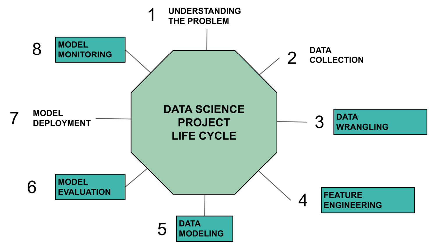
Figure 1.1 – The steps in a data science project life cycle, highlighting where Comet is involved in green rectangles

The steps involved include the following:

• Data wrangling – thanks to the integration with some popular libraries for data visualization, such as the matplotlib, plotly, and PIL Python libraries, we can build panels in Comet to perform EDA, which can be used as a preliminary step for data wrangling. We will describe the concept of a panel in more detail in the next sections and chapters of this book.
• Feature engineering – Comet provides an easy way to track different experiments, which can be compared to select the best input feature sets.
• Data modeling – Comet can be used to debug your models, as well as performing hyperparameter tuning, thanks to the concept of Optimizer. We will illustrate how to work with Comet Optimizer in the next chapters of this book.
• Model evaluation – Comet provides different tools to evaluate a model, including panels, evaluation metrics extracted from each experiment, and the possibility to compare different experiments.
• Model monitoring – Once a model has been deployed, you can continue to track it in Comet with the previously described tools. Comet also provides an external service, named Model Production Monitoring (MPM), that permits us to monitor the performance of a model in real time. The MPM service is not included in the Comet free plan.

We cannot exploit Comet directly to deploy a model. However, we can easily integrate Comet with GitLab, one of the most famous DevOps platforms. We will discuss the integration between Comet and GitLab in Chapter 7, Extending the GitLab DevOps Platform with Comet.

To summarize, Comet provides a single point of access to almost all the steps in a data science project, thanks to the different tools and features provided. With respect to a traditional and manual pipeline, Comet permits automating and reducing error propagation during the whole data science process.

Now that you are familiar with why and when to use Comet, we can move on to looking at the purpose of Comet.

Purpose

The main objective of Comet is to provide users with a platform where they can do the following:

• Organize your project into different experiments – This is useful when you want to try different strategies or algorithms or produce different models.
• Track, reproduce, and store experiments – Comet assigns to each experiment a unique identifier; thus, you can track every single change in your code without worrying about recording the changes you make. In fact, Comet also stores the code used to run each experiment.
• Share your projects and experiments with other collaborators – You can invite other members of your team to read or modify your experiments, thus making it easy to extract insights from data or to choose the best model for a given problem.

Now that you have learned about the purpose of Comet, we can illustrate how to access the Comet platform for the first time.

First access to the Comet platform

Using Comet requires the creation of an account on the platform. The Comet platform is available at this link: https://www.comet.ml/. Comet provides different plans that depend on your needs. In the free version, you can have access to almost all the features, but you cannot share your projects with your collaborators.

If you are an academic, you can create a premium Comet account for free, by following the procedure for academics: https://www.comet.ml/signup?plan=academic. In this case, you must provide your academic account.

You can create a free account simply by clicking on the Create a Free Account button and following the procedure.

Comet has a nested architecture, as shown in the following figure:

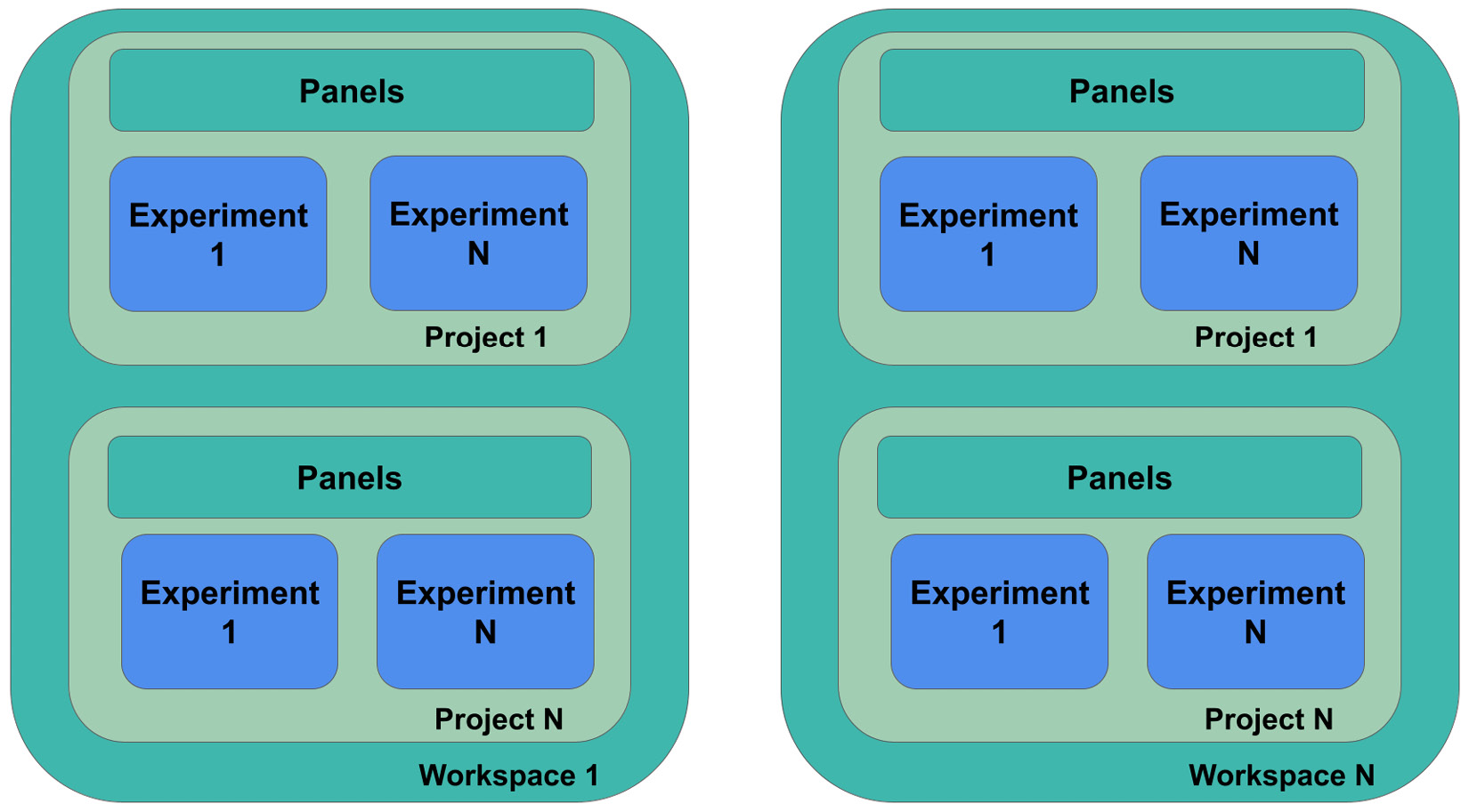
Figure 1.2 – The modular architecture in Comet

The main components of the Comet architecture include the following:

• Workspaces
• Projects
• Experiments
• Panels

Let's analyze each component separately, starting with the first one – workspaces.

Workspaces

A Comet workspace is a collection of projects, private or shared with your collaborators. When you create your account, Comet creates a default workspace, named with your username. However, you can create as many workspaces as you want and share them with different collaborators.

To create a new workspace, we can perform the following operations:

1. Click on your username on the left side of the page on the dashboard.
2. Select Switch Workspace | View all Workspaces.
3. Click on the Create a workspace button.
4. Enter the workspace name, which must be unique across the whole platform. We suggest prepending your username to the workspace name, thus avoiding conflicting names.
5. Click the Save button.

The following figure shows an account with two workspaces:

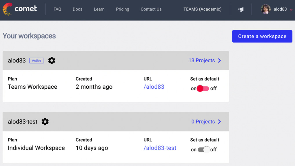
Figure 1.3 – An account with two workspaces

In the example, there are two workspaces, alod83, which is the default and corresponds to the username, and alod83-test.

Now that we have learned how to create a workspace, we can move on to the next feature: projects.

Projects

A Comet project is a collection of experiments. A project can be either private or public. A private project is visible only by the owner and their collaborator, while a public project can be seen by everyone.

In Comet, you can create as many projects as you want. A project is identified by a name and can belong only to a workspace, and you cannot move a project from one workspace to another.

To create a project, we perform the following operations:

1. Launch the browser and go to https://www.comet.ml/.
2. If you have not already created an account, click on the top-right Create a free account button and follow the procedure. If you already have an account, jump directly to step 3.
3. Log in to the platform by clicking the Login button located in the top-right part of the screen.
4. Select a Workspace.
5. Click on the new project button in the top-right corner of the screen.
6. A new window opens where you can enter the project information, as shown in the following figure:

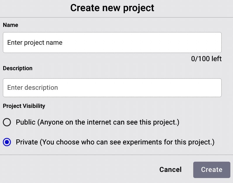
Figure 1.4 – The Create new project window

The window contains three sections: Name, where you write the project name, Description, a text box where you can provide a summary of the project, and Project Visibility, where you can decide to make the project either private or public. Enter the required information.

7. Click on the Create button.

The following figure shows the just-created Comet dashboard:

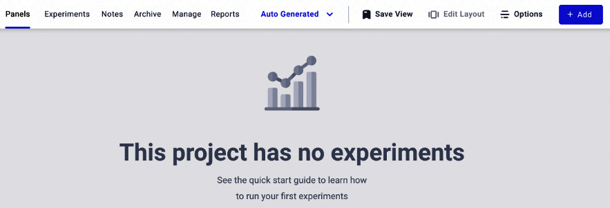
Figure 1.5 – A screenshot of an empty project in Comet

The figure shows the empty project, with a top menu where you can start adding objects.

Experiments

A Comet experiment is a process that tracks how some defined variables vary while changing the underlying conditions. An example of an experiment is hyperparameter tuning in a machine learning project. Usually, an experiment should include different runs that test different conditions.

Comet defines the Experiment class to track experiments. All the experiments are identified by the same API key. Comet automatically generates an API key. However, if for some reason you need to generate a new API key, you can perform the following steps:

1. Click on your username on the left side of the page on the dashboard.
2. Select Settings from the menu.
3. Under the Developer Information section, click Generate API Key. This operation will override the current API key.
4. Click Continue on the pop-up window. You can copy the value of the new API key by clicking on the API Key button.

We can add an experiment to a project by taking the following steps:

1. Click on the Add button, located in the top-right corner.
2. Select New Experiment from the menu.
3. Copy the following code (Ctrl + C on Windows/Linux environments or Cmd + C on macOS) and then click on the Done button:

   # import comet-ml at the top of your file
   from comet-ml import Experiment
   # Create an experiment with your api key
   experiment = Experiment(
       api_key="YOUR API KEY",
       project_name="YOUR PROJECT NAME",
       workspace="YOUR WORKSPACE",
   )

The previous code creates an experiment in Comet. Comet automatically sets the api_key, project_name, and workspace variables. We can paste the previous code after the code we have already written to load and clean the dataset.

In general, storing an API key in code is not secure, so Comet defines two alternatives to store the API key. Firstly, in a Unix-like console, create an environment variable called COMET_API_KEY, as follows:

export COMET_API_KEY="YOUR-API-KEY"

Then, you can access it from your code:

import os
API_KEY = os.environ['COMET_API_KEY']

The previous code uses the os package to extract the COMET_API_KEY environment variable.

As a second alternative, we can define a .comet.config file and put it in our home directory or our current directory and store the API key, as follows:

[comet]
api_key=YOUR-API-KEY
project_name=YOUR-PROJECT-NAME,
workspace=YOUR-WORKSPACE

Note that the variable values should not be quoted or double-quoted. In this case, when we create an experiment, we can do so as follows:

experiment = Experiment()

We can use the Experiment class to track DataFrames, models, metrics, figures, images, metrics, and artifacts. For each element to be tracked, the Experiment class provides a specific method. Every tracking function starts with log_. Thus, we have log_metric(), log_model(), log_image(), and so on.

To summarize it in one sentence, experiments are the bridge between your code and the Comet platform.

Experiments can also be used as context managers, for example, to split the training and test phases into two different contexts. We will discuss these aspects in more detail in Chapter 3, Model Evaluation in Comet.

Now that you are familiar with Comet experiments, we can describe the next element – panels.

Panels

A Comet panel is a visual display of data. It can be either static or interactive. You can choose whether to make a panel private, share it with your collaborators, or make it public. While charts refer to a single experiment, panels can display data across different experiments, so we can define a panel only within the Comet platform and not in our external code.

Comet provides different ways to build a panel:

• Use a panel template.
• Write a custom panel in Python.
• Write a custom panel in JavaScript.

Let's analyze the three ways separately, starting with the first one: Use a panel template.

From the main page of our project, we can perform the following operations:

1. Click on the Add button located in the top-right corner of the page.
2. Select New Panel.
3. Choose the panel and select Add in the new window, as shown in the following figure:

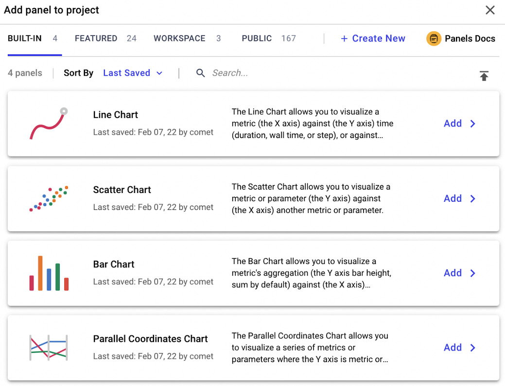
Figure 1.6 – The main window to add a panel in Comet

The figure shows the different types of available panels, divided into four main categories, identified by the top menu:

• BUILT-IN – Comet provides some basic panels.
• FEATURED – The most popular panels implemented by the Comet community and made available to everyone.
• WORKSPACE – Your private panels, if any.
• PUBLIC – All the public panels implemented by Comet users.

We can configure a built-in panel by setting some parameters in the Comet interface, as shown in the following figure:

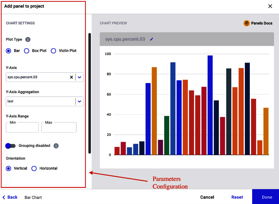
Figure 1.7 – Parameter configuration in a built-in Comet panel

The figure shows the form for parameter configuration on the left and a preview of the panel on the right.

While we can configure built-in panels through the Comet interface, we need to write some code to use the other categories of panels – featured, workspace, and public. In these cases, we select the type of panel, and then we configure the associated parameters, in the form of key-value pairs, as shown in the following figure:

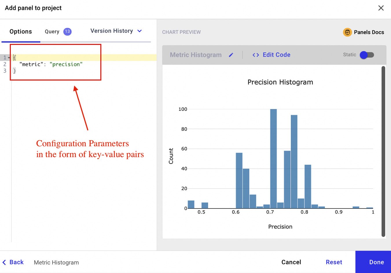
Figure 1.8 – Parameters configuration in a featured, workspace, or public panel

On the left, the figure shows a text box, where we can insert the configuration parameters in the form of a Python dictionary:

{"key1" : "value1",
 "key2" : "value2", 
 "keyN" : "valueN"
}

Note the double quotes for the strings. The key-value pairs depend on the specific panel.

The previous figure also shows a preview of the panel on the right, with the possibility to access the code that generates the panel directly, through the Edit Code button.

So far, we have described how to build a panel through an existing template. Comet also provides the possibility to write custom panels in Python or JavaScript. We will describe this advanced feature in the next chapter, on EDA in Comet.

Now that you are familiar with the Comet basic concepts, we can implement two examples that use Comet:

• Tracking images in Comet
• Building a panel in Comet

Let's start with the first use case – tracking images in Comet.

For the first use case, we describe how to build a panel showing a time series related to some Italian performance indicators in Comet. The example uses the matplotlib library to build the graphs.

You can download the full code of this example from the official GitHub repository of the book, available at the following link: https://github.com/PacktPublishing/Comet-for-Data-Science/tree/main/01.

The dataset used is provided by the World Bank under the CC 4.0 license, and we can download it from the following link: https://api.worldbank.org/v2/en/country/ITA?downloadformat=csv.

The dataset contains more than 1,000 time series indicators regarding the performance of Italy's economy. Among them, we will focus on the 52 indicators related to Gross Domestic Product (GDP), as shown in the following table:

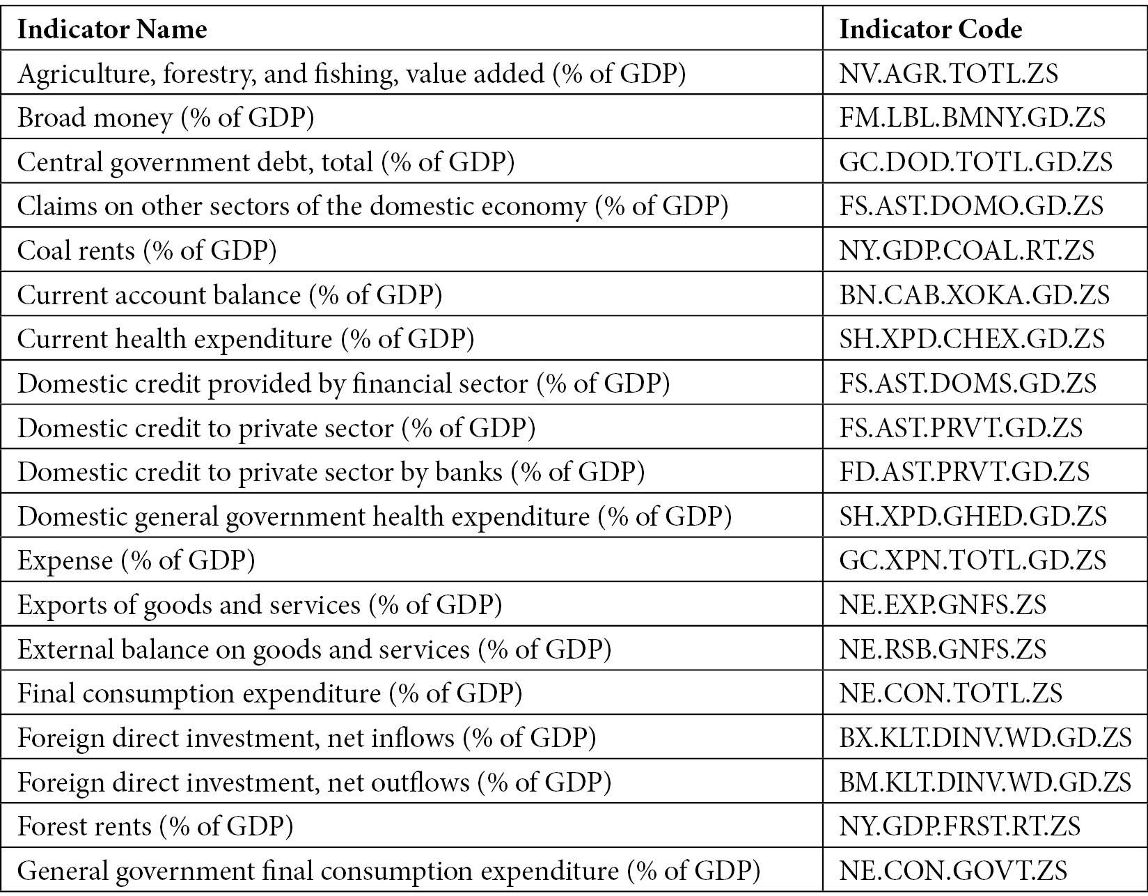
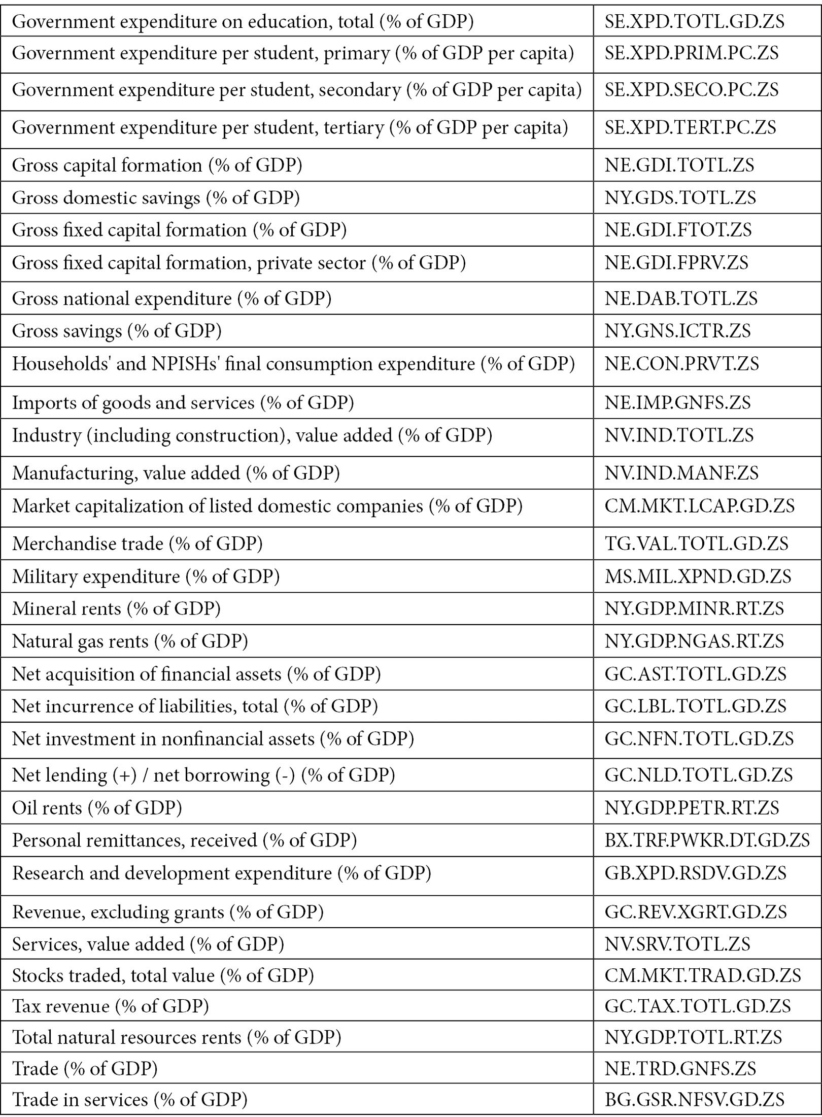
Figure 1.9 – Time series indicators related to GDP used to build the dashboard in Comet

The table shows the indicator name and its associated code.

We implement the Comet dashboard through the following steps:

1. Download the dataset.
2. Clean the dataset.
3. Build the visualizations.
4. Integrate the graphs in Comet.
5. Build a panel.

So, let's move on to building your first use case in Comet, starting with the first steps, downloading and cleaning the dataset.

Downloading the dataset

As already said at the beginning of this section, we can download the dataset from this link: https://api.worldbank.org/v2/en/country/ITA?downloadformat=csv. Before we can use it, we must remove the first two lines from the file, because they are simply a header section. We can perform the following steps:

1. Download the dataset from the previous link.
2. Unzip the downloaded folder.
3. Enter the unzipped directory and open the file named API_ITA_DS2_en_csv_v2_3472313.csv with a text editor.
4. Select and remove the first four lines, as shown in the following figure:

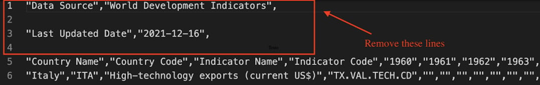
Figure 1.10 – Lines to be removed from the API_ITA_DS2_en_csv_v2_3472313.csv file

5. Save and close the file. Now, we are ready to open and prepare the dataset for the next steps. Firstly, we load the dataset as a pandas DataFrame:

   import pandas as pd
   df = pd.read_csv('API_ITA_DS2_en_csv_v2_3472313.csv') 

We import the pandas library, and then we read the CSV file through the read_csv() method provided by pandas.

The following figure shows an extract of the table:

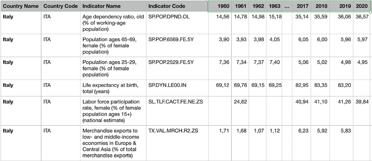
Figure 1.11 – An extract of the API_ITA_DS2_en_csv_v2_3472313.csv dataset

The dataset contains 66 columns, including the following:

• Country Name – Set to Italy for all the records.
• Country Code – Set to ITA for all the records.
• Indicator Name – Text describing the name of the indicator.
• Indicator Code – String specifying the unique code associated with the indicator.
• Columns from 1960 to 2020 – The specific value for a given indicator in that specific year.
• Empty column – An empty column. The pandas DataFrame names this column Unnamed: 65.

Now that we have downloaded and loaded the dataset as a pandas DataFrame, we can perform dataset cleaning.

Dataset cleaning

The dataset presents the following problems:

• Some columns are not necessary for our purpose.
• We need only indicators related to GDP.
• The dataset contains the years' names in the header.
• Some rows contain missing values.

We can solve the previous problems by cleaning the dataset with the following operations:

• Drop unnecessary columns.
• Filter only GDP-based indicators.
• Transpose the dataset to obtain years as a single column.
• Deal with missing values.

Now, we can start the data cleaning process from the first step – drop unnecessary columns. We should remove the following columns:

• Country Name
• Country Code
• Indicator Code
• Unnamed: 65

We can perform this operation with a single line of code, as follows:

df.drop(['Country Name', 'Country Code', 'Indicator Code','Unnamed: 65'], axis=1, inplace = True)

The previous code exploits the drop() method of the pandas DataFrame. As the first parameter, we pass the list of columns to be dropped. The second parameter, (axis = 1), specifies that we want to drop columns, and the last parameter, (inplace = True), specifies that all the changes must be stored in the original dataset.

Now that we have removed unnecessary columns, we can filter only GDP-based indicators. All the GDP-based indicators contain the following text: (% of GDP). So, we can select only these indicators by searching all the records where the Indicator Name column contains that text, as shown in the following piece of code:

df = df[df['Indicator Name'].str.contains('(% of GDP)')]

We can use the operation contained in square brackets (df['Indicator Name'].str.contains('(% of GDP)')) to extract only the rows that match our criteria, in this case, the rows that contain the string (% of GDP). We have exploited the str attribute of the DataFrame to extract all the strings of the Indicator Name column, and then we have matched each of them with the string (% of GDP). The contains() method returns True only if there is a match; otherwise, it returns False.

Now we have only the interesting metrics. So, we can move on to the next step: transposing the dataset to obtain years as a single column. We can perform this operation as follows:

df = df.transpose()
df.columns = df.iloc[0] 
df = df[1:]

The transpose() method exchanges rows and columns. In addition, in the transposed DataFrame, we want to rename the columns to the indicator name. We can achieve this through the last two lines of code.

Now that we have transposed the dataset, we can proceed with missing values management. We could adopt different strategies, such as interpolation or average values. However, to keep the example simple, we decide to simply drop rows from 1960 to 1969 that do not contain values for almost all the analyzed indicators. In addition, we drop the indicators that contain less than 30 no-null values.

We can perform these operations through the following line of code:

df.dropna(thresh=30, axis=1, inplace = True)
df = df.iloc[10:]

Firstly, we drop all the columns (each representing a different indicator) with less than 30 non-null values. Then, we drop all the rows from 1960 to 1969.

Now, the dataset is cleaned and ready for further analysis. The following figure shows an extract of the final dataset:

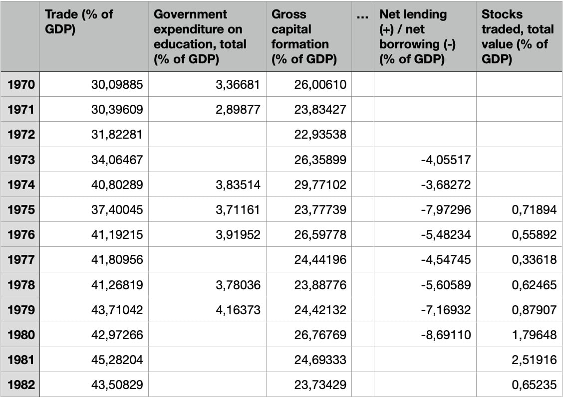
Figure 1.12 – The final dataset, after the cleaning operations

The figure shows that we have grouped years from different columns into a single column, as well as splitting indicators from one column into different columns. Before the dropping operation, the dataset before had 61 rows and 52 columns. After dropping, the resulting dataset has 51 rows and 39 columns.

We can save the final dataset, as follows:

df.to_csv('API_IT_GDP.csv')

We have exploited the to_csv() method provided by the pandas DataFrame.

Now that we have cleaned the dataset, we can move on to the next step – building the visualizations.

Building the visualizations

For each indicator, we build a separate graph that represents its trendline over time. We exploit the matplotlib library.

Firstly, we define a simple function that plots an indicator and saves the figure in a file:

import matplotlib.pyplot as plt
import numpy as np
def plot_indicator(ts, indicator):
    xmin = np.min(ts.index)
    xmax = np.max(ts.index)
    plt.xticks(np.arange(xmin, xmax+1, 1),rotation=45)
    plt.xlim(xmin,xmax)
    plt.title(indicator)
    plt.grid()
    plt.figure(figsize=(15,6))
    plt.plot(ts)
    fig_name = indicator.replace('/', "") + '.png'
    plt.savefig(fig_name)
    return fig_name

The plot_indicator() function receives a time series and the indicator name as input. Firstly, we set the range of the x axis through the xticks() method. Then, we set the title through the title() method. We also activate the grid through the grid() method, as well as setting the figure size, through the figure() method. Finally, we plot the time series (plt.plot(ts)) and save it to our local filesystem. If the indicator name contains a /, we replace it with an empty value. The function returns the figure name.

The previous code generates a figure like the following one:

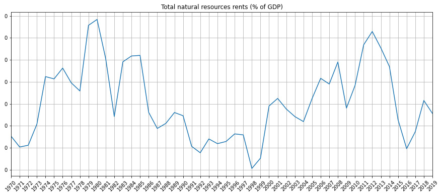
Figure 1.13 – An example of a figure generated by the plot_indicator() function

Now that we have set up the code to create the figures, we can move on to the last step: integrating the graphs in Comet.

Integrating the graphs in Comet

Now, we can create a project and an experiment by following the procedure described in the Getting started with workspaces, projects, experiments, and panels section. We copy the generated code and paste it into our script:

from comet-ml import Experiment
experiment = Experiment()

We have just created an experiment. We have stored the API key and the other parameters in the .comet.config file located in our working directory.

Now we are ready to plot the figures. We use the log_image() method provided by the Comet experiment to store every produced figure in Comet:

for indicator in df.columns:
    ts = df[indicator]
    ts.dropna(inplace=True)
    ts.index = ts.index.astype(int)
    fig = plot_indicator(ts,indicator)
    experiment.log_image(fig,name=indicator, image_format='png')

We iterate over the list of indicators, identified by the DataFrame columns (df.columns). Then, we extract the associated time series from the current indicator. After, we save the figure through the plot_indicator() function, previously defined. Finally, we load the image in Comet.

The code is complete, so we run it.

When the running phase is complete, the results of the experiments are available in Comet. To see the produced graphs, we perform the following steps:

1. Open your Comet project.
2. Select Experiments from the top menu.
3. A table with all the experiments that have run appears. In our case, there is only one experiment.
4. Click on the experiment name, in the first cell on the left. Since we have not set a specific name for the experiment, Comet will add it for us. An example of a name given by Comet is straight_contract_1272.
5. Comet shows a dashboard with all the experiment details. Click on the Graphics section from the left menu. Comet shows all your produced graphs, as shown in the following figure:

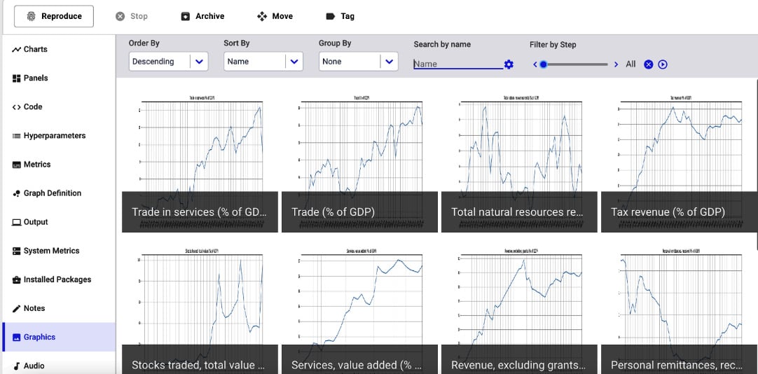
Figure 1.14 – A screenshot of the Graphics section

The figure shows all the indicators in descending order. Alternatively, you can display figures in ascending order and you can sort and group them.

Comet also stores the original images under the Assets & Artifacts section of the left menu, as shown in the following figure:

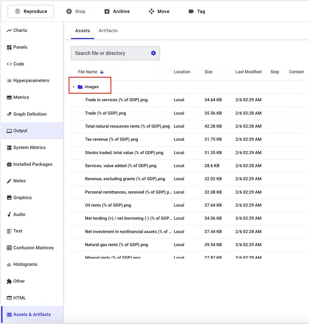
Figure 1.15 – A screenshot of the Assets & Artifacts section

The figure shows that all the images are stored in the images directory. The Assets & Artifacts directory also contains two directories, named notebooks and source-code.

Finally, the Code section shows the code that has generated the experiment. This is very useful when running different experiments.

Now that you have learned how to track images in Comet, we can build a panel with the created images.

Building a panel

To build the panel that shows all the tracked images, you can use the Show Images panel, which is available on the Featured Panels tab of the Comet panels. To add this panel, we perform the following steps:

1. From the Comet main dashboard, click on the Add button in the top-right corner.
2. Select New Panel.
3. Select the Featured tab | Show Images | Add.

A new window opens, as shown in the following figure:

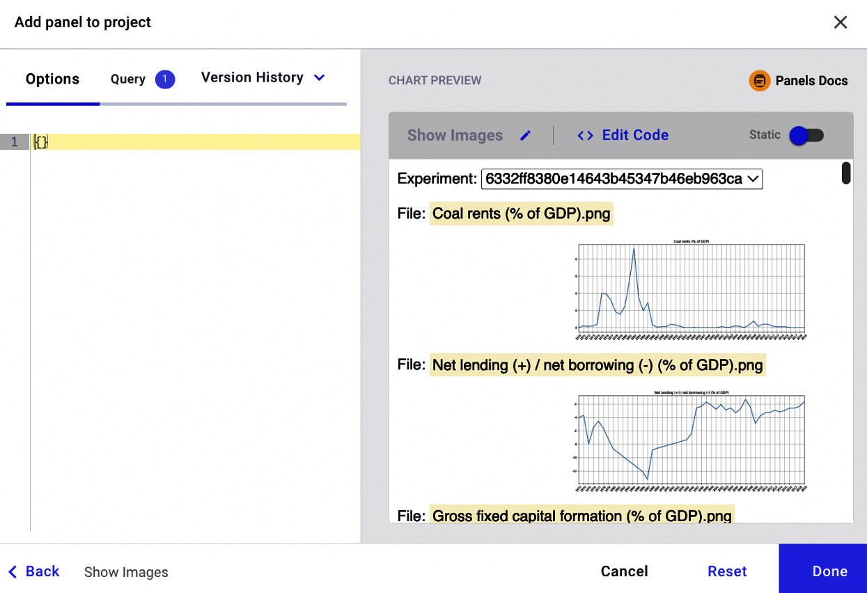
Figure 1.16 – The interface to build the Featured Panel called Show Images

The figure shows a preview of the panel with all the images. We can set some variables, through the key-value pairs, that contain only one image, by specifying the following parameters in the left text box:

{  "imageFileName": "Gross fixed capital formation (% of GDP).png" }

The "imageFileName" parameter allows us to specify exactly the image to be plotted. The following figure shows a preview of the resulting panel, after specifying the image filename:

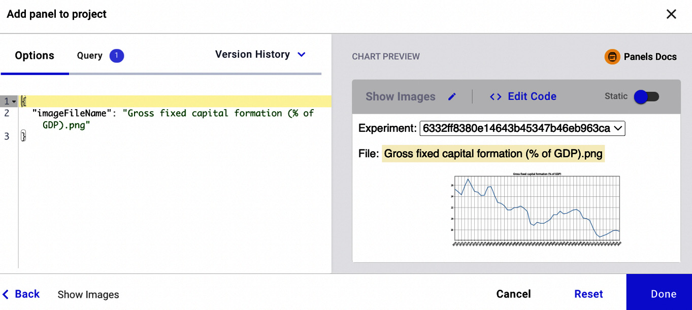
Figure 1.17 – A preview of the Show Images panel after specifying key-value pairs

The figure shows how we can manipulate the output of the panel on the basis of the key-value variables. The variables accepted by a panel depend on the specific panel. We will investigate this aspect more deeply in the next chapter.

Now that we have learned how to get started with Comet, we can move on to a more complex example that implements a simple linear regression model.

The objective of this example is to show how to log a metric in Comet. In detail, we set up an experiment that calculates the different values of Mean Squared Error (MSE) produced by fitting a linear regression model with different training sets. Every training set is derived from the same original dataset, by specifying a different seed.

You can download the full code of this example from the official GitHub repository of the book, available at the following link: https://github.com/PacktPublishing/Comet-for-Data-Science/tree/main/01.

We use the scikit-learn Python package to implement a linear regression model. For this use case, we will use the diabetes dataset, provided by scikit-learn.

We organize the experiment in three steps:

• Initialize the context.
• Define, fit, and evaluate the model.
• Show results in Comet.

Let's start with the first step: initializing the context.

Initializing the context

Firstly, we create a .comet.config file in our working directory, as explained in the Getting started with workspaces, projects, experiments, and panels, in the Experiment section.

As the first statement of our code, we create a Comet experiment, as follows:

from comet-ml import Experiment
experiment = Experiment()

Now, we load the diabetes dataset, provided by scikit-learn, as follows:

from sklearn.datasets import load_diabetes
 diabetes = load_diabetes()
X = diabetes.data
y = diabetes.target

We load the dataset and stored data and target in X and y variables, respectively.

Our context is now ready, so we can move on to the second part of our experiment: defining, fitting, and evaluating the model.

Defining, fitting, and evaluating the model

Let's start with the imports:

1. Firstly, we import all the libraries and functions that we will use:

   import numpy as np
   from sklearn.model_selection import train_test_split
   from sklearn.linear_model import LinearRegression
   from sklearn.metrics import mean_squared_error

We import NumPy, which we will use to build the array of different seeds, and other scikit-learn classes and methods used for the modeling phase.

2. We set the seeds to test, as follows:

   n = 100
   seed_list = np.arange(0, n+1, step = 5)

We define 20 different seeds, ranging from 0 to 100, with a step of 5. Thus, we have 0, 5, 10, 15 … 95, 100.

3. For each seed, we extract a different training and test set, which we use to train the same model, calculate the MSE, and log it in Comet, using the following code:

   for seed in seed_list:
       X_train, X_test, y_train, y_test = train_test_split(X, y, test_size=0.20, random_state=seed)
       model = LinearRegression()
       model.fit(X_train,y_train)
       y_pred = model.predict(X_test)
       mse = mean_squared_error(y_test,y_pred)
       experiment.log_metric("MSE", mse, step=seed)

In the previous code, firstly we split the dataset into training and test sets, using the current seed. We reserve 20% of the data for the test set and the remaining 80% for the training set. Then, we build the linear regression model, we fit it (model.fit()), and we predict the next values for the test set (model.predict()). We also calculate MSE through the mean_squared_error() function. Finally, we log the metric in Comet through the log_metric() method. The log_metric() method receives the metric name as the first parameter and the metric value as the second parameter. We also specify the step for the metric that corresponds to the seed, in our case.

Now, we can launch the code and see the results in Comet.

Showing results in Comet

To see the results in Comet, we perform the following steps:

1. Open your Comet project.
2. Select Experiments from the top menu.
3. The dashboard shows a list of all the experiments. In our case, there is just one experiment.
4. Click on the experiment name, in the first cell on the left. Since we have not set the experiment name, Comet has set the experiment name for us. Comet shows a dashboard with all the experiment details.

In our experiment, we can see some results in three different sections: Charts, Metrics, and System Metrics.

Under the Charts section, Comet shows all the graphs produced by our code. In our case, there is only one graph referring to MSE, as shown in the following figure:

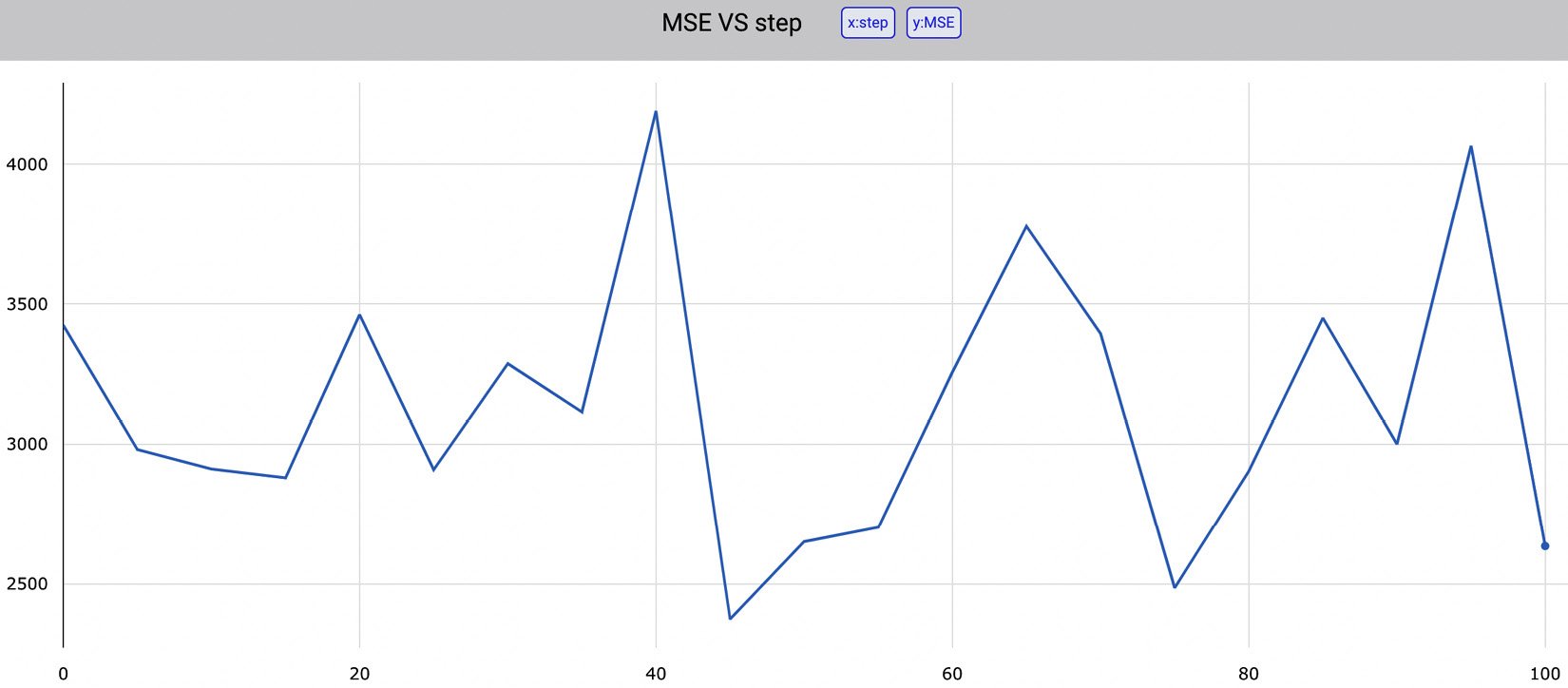
Figure 1.18 – The value of MSE for different seeds provided as input to train_test_split()

The figure shows how the value of MSE depends on the seed value provided as input to the train_test_split() function. The produced graph is interactive, so we can view every single value in the trend line. We can download all the graphs as .jpeg or .svg files. In addition, we can download as a .json file of the data that has generated the graph. The following piece of code shows the generated JSON:

[{"x": [0,5,10,15,20,25,30,35,40,45,50,55,60,65,70,75,80,85,90,95],
"y":[3424.3166882137334,2981.5854714667616,2911.8279516891607,2880.7211416534115,3461.6357411723743,2909.472185919797,3287.490246176432,3115.203798301772,4189.681600195272,2374.3310824431856,2650.9384531241985,2702.2483323059314,3257.2142019316807,3776.092087838954,3393.8576719100192,2485.7719017765257,2904.0610865479025,3449.620077951196,3000.56755060663,4065.6795384526854],
"type":"scattergl",
"name":"MSE"}]

The previous code shows that there are two variables, x and y, and that the type of graph is scattergl.

Under the Metrics section, Comet shows a table with all the logged metrics, as shown in the following figure:

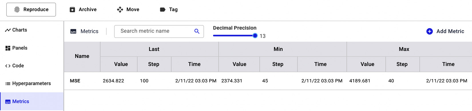
Figure 1.19 – The Metrics section in Comet

For each metric, Comet shows the last, minimum, and maximum values, as well as the step that determined those values.

Finally, under the System Metrics section, Comet shows some metrics about the system conditions, including memory usage and CPU utilization, as well as the Python version and the type of operating system, as shown in the following figure:

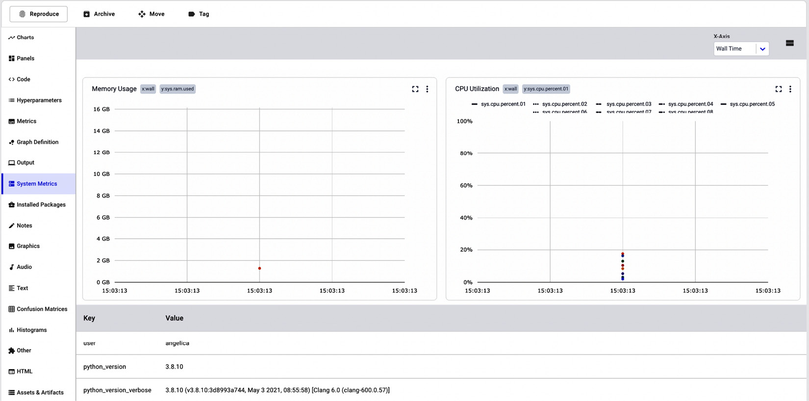
Figure 1.20 – System Metrics in Comet

The System Metrics section shows two graphs, one for memory usage (on the left in the figure) and the other for the CPU utilization (on the right in the figure). Under the graph, the System Metrics section also shows a table with other useful information regarding the machine that generated the experiment.

We just completed our first steps in the journey of getting started with Comet!

Throughout this chapter, we described the motivation and purpose of the Comet platform, as well as how to get started with it. We showed that Comet can be used in almost all the steps of a data science project.

We also illustrated the concepts of workspaces, projects, experiments, and panels, and we set up the environment to work with Comet. Finally, we implemented two practical examples to get familiar with Comet.

Now that you have learned the basic concepts and we have set up the environment, we can move on to more specific and complex features provided by Comet.

In the next chapter, we will review some concepts about EDA and how to perform it in Comet.

• Grus, J. (2019). Data Science from Scratch: First Principles with Python. O'Reilly Media.
• Prevos, P. (2019). Principles of Strategic Data Science: Creating value from data, big and small. Packt Publishing Ltd.