


 Download code from GitHub
Predicting the cost, and hence the severity, of claims in an insurance company is a real-life problem that needs to be solved in an accurate way. In this chapter, we will show you how to develop a predictive model for analyzing insurance severity claims using some of the most widely used regression algorithms.
We will start with simple linear regression (LR) and we will see how to improve the performance using some ensemble techniques, such as gradient boosted tree (GBT) regressors. Then we will look at how to boost the performance with Random Forest regressors. Finally, we will show you how to choose the best model and deploy it for a production-ready environment. Also, we will provide some background studies on machine learning workflow, hyperparameter tuning, and cross-validation.
For the implementation, we will use Spark ML API for faster computation and massive scalability. In a nutshell, we will learn the following topics throughout this end-to-end project:
- Machine learning and learning workflow
- Hyperparameter tuning and cross-validation of ML models
- LR for analyzing insurance severity claims
- Improving performance with gradient boosted regressors
- Boosting the performance with random forest regressors
- Model deployment
Machine learning (ML) is about using a set of statistical and mathematical algorithms to perform tasks such as concept learning, predictive modeling, clustering, and mining useful patterns can be performed. The ultimate goal is to improve the learning in such a way that it becomes automatic, so that no more human interactions are needed, or to reduce the level of human interaction as much as possible.
We now refer to a famous definition of ML by Tom M. Mitchell (Machine Learning, Tom Mitchell, McGraw Hill, 1997), where he explained what learning really means from a computer science perspective:
"A computer program is said to learn from experience E with respect to some class of tasks T and performance measure P, if its performance at tasks in T, as measured by P, improves with experience E."
Based on the preceding definition, we can conclude that a computer program or machine can do the following:
- Learn from data and histories
- Be improved with experience
- Interactively enhance a model that can be used to predict an outcome
A typical ML function can be formulated as a convex optimization problem for finding a minimizer of a convex function f that depends on a variable vector w (weights), which has d records. Formally, we can write this as the following optimization problem:

Here, the objective function is of the form:

Here, the vectors

are the training data points for 1≤i≤n, and are their corresponding labels that we want to predict eventually. We call the method linear if L(w;x,y) can be expressed as a function of wTx and y.
The objective function f has two components:
- A regularizer that controls the complexity of the model
- The loss that measures the error of the model on the training data
The loss function L(w;) is typically a convex function in w. The fixed regularization parameter λ≥0 defines the trade-off between the two goals of minimizing the loss on the training error and minimizing model complexity to avoid overfitting. Throughout the chapters, we will learn in details on different learning types and algorithms.
On the other hand, deep neural networks (DNN) form the core of deep learning (DL) by providing algorithms to model complex and high-level abstractions in data and can better exploit large-scale datasets to build complex models
There are some widely used deep learning architectures based on artificial neural networks: DNNs, Capsule Networks, Restricted Boltzmann Machines, deep belief networks, factorization machines and recurrent neural networks.
These architectures have been widely used in computer vision, speech recognition, natural language processing, audio recognition, social network filtering, machine translation, bioinformatics and drug design. Throughout the chapters, we will see several real-life examples using these architectures to achieve state-of-the art predictive accuracy.
A typical ML application involves several processing steps, from the input to the output, forming a scientific workflow as shown in Figure 1, ML workflow. The following steps are involved in a typical ML application:
- Load the data
- Parse the data into the input format for the algorithm
- Pre-process the data and handle the missing values
- Split the data into three sets, for training, testing, and validation (train set and validation set respectively) and one for testing the model (test dataset)
- Run the algorithm to build and train your ML model
- Make predictions with the training data and observe the results
- Test and evaluate the model with the test data or alternatively validate the model using some cross-validator technique using the third dataset called a validation dataset
- Tune the model for better performance and accuracy
- Scale up the model so that it can handle massive datasets in future
- Deploy the ML model in production:

Figure 1: ML workflow
The preceding workflow is represent a few steps to solve ML problems. Where, ML tasks can be broadly categorized into supervised, unsupervised, semi-supervised, reinforcement, and recommendation systems. The following Figure 2, Supervised learning in action, shows the schematic diagram of supervised learning. After the algorithm has found the required patterns, those patterns can be used to make predictions for unlabeled test data:

Figure 2: Supervised learning in action
Examples include classification and regression for solving supervised learning problems so that predictive models can be built for predictive analytics based on them. Throughout the upcoming chapters, we will provide several examples of supervised learning, such as LR, logistic regression, random forest, decision trees, Naive Bayes, multilayer perceptron, and so on.
A regression algorithm is meant to produce continuous output. The input is allowed to be either discrete or continuous:

Figure 3: A regression algorithm is meant to produce continuous output
A classification algorithm, on the other hand, is meant to produce discrete output from an input of a set of discrete or continuous values. This distinction is important to know because discrete-valued outputs are handled better by classification, which will be discussed in upcoming chapters:

Figure 4: A classification algorithm is meant to produce discrete output
In this chapter, we will mainly focus on the supervised regression algorithms. We will start with describing the problem statement and then we move on to the very simple LR algorithm. Often, performance of these ML models is optimized using hyperparameter tuning and cross-validation techniques. So knowing them, in brief, is mandatory so that we can easily use them in future chapters.
Tuning an algorithm is simply a process that one goes through in order to enable the algorithm to perform optimally in terms of runtime and memory usage. In Bayesian statistics, a hyperparameter is a parameter of a prior distribution. In terms of ML, the term hyperparameter refers to those parameters that cannot be directly learned from the regular training process.
Hyperparameters are usually fixed before the actual training process begins. This is done by setting different values for those hyperparameters, training different models, and deciding which ones work best by testing them. Here are some typical examples of such parameters:
- Number of leaves, bins, or depth of a tree
- Number of iterations
- Number of latent factors in a matrix factorization
- Learning rate
- Number of hidden layers in a deep neural network
- The number of clusters in k-means clustering and so on
In short, hyperparameter tuning is a technique for choosing the right combination of hyperparameters based on the performance of presented data. It is one of the fundamental requirements for obtaining meaningful and accurate results from ML algorithms in practice. The following figure shows the model tuning process, things to consider, and workflow:

Figure 5: Model tuning process
Cross-validation (also known as rotation estimation) is a model validation technique for assessing the quality of the statistical analysis and results. The target is to make the model generalized toward an independent test set. It will help if you want to estimate how a predictive model will perform accurately in practice when you deploy it as an ML application. During the cross-validation process, a model is usually trained with a dataset of a known type.
Conversely, it is tested using a dataset of an unknown type. In this regard, cross-validation helps to describe a dataset to test the model in the training phase using the validation set. There are two types of cross-validation that can be typed as follows:
In most cases, the researcher/data scientist/data engineer uses 10-fold cross-validation instead of testing on a validation set (see more in Figure 6, 10-fold cross-validation technique). This is the most widely used cross-validation technique across all use cases and problem types, as explained by the following figure.
Basically, using this technique, your complete training data is split into a number of folds. This parameter can be specified. Then the whole pipeline is run once for every fold and one ML model is trained for each fold. Finally, the different ML models obtained are joined by a voting scheme for classifiers or by averaging for regression:

Figure 6: 10-fold cross-validation technique
Moreover, to reduce the variability, multiple iterations of cross-validation are performed using different partitions; finally, the validation results are averaged over the rounds.
Predicting the cost, and hence the severity, of claims in an insurance company is a real-life problem that needs to be solved in a more accurate and automated way. We will do something similar in this example.
We will start with simple logistic regression and will learn how to improve the performance using some ensemble techniques, such as an random forest regressor. Then we will look at how to boost the performance with a gradient boosted regressor. Finally, we will show how to choose the best model and deploy it for a production-ready environment.
When someone is devastated by a serious car accident, his focus is on his life, family, child, friends, and loved ones. However, once a file is submitted for the insurance claim, the overall paper-based process to calculate the severity claim is a tedious task to be completed.
This is why insurance companies are continually seeking fresh ideas to improve their claims service for their clients in an automated way. Therefore, predictive analytics is a viable solution to predicting the cost, and hence severity, of claims on the available and historical data.
A dataset from the Allstate Insurance companywill be used, which consists of more than 300,000 examples with masked and anonymous data and consisting of more than 100 categorical and numerical attributes, thus being compliant with confidentiality constraints, more than enough for building and evaluating a variety of ML techniques.
The dataset is downloaded from the Kaggle website at https://www.kaggle.com/c/allstate-claims-severity/data. Each row in the dataset represents an insurance claim. Now, the task is to predict the value for the loss column. Variables prefaced with cat are categorical, while those prefaced with cont are continuous.
It is to be noted that the Allstate Corporation is the second largest insurance company in the United States, founded in 1931. We are trying to make the whole thing automated, to predict the cost, and hence the severity, of accident and damage claims.
Let's look at some data properties (use the EDA.scala file for this). At first, we need to read the training set to see the available properties. To begin with, let's place your training set in your project directory or somewhere else and point to it accordingly:
val train = "data/insurance_train.csv"I hope you have Java, Scala and Spark installed and configured on your machine. If not, please do so. Anyway, I'm assuming they are. So let's create an active Spark session, which is the gateway for any Spark application:
val spark = SparkSessionCreate.createSession()
import spark.implicits._
Note
Spark session alias on Scala REPL:
If you are inside Scala REPL, the Spark session alias spark is already defined, so just get going.
Here, I have a method called createSession() under the class SparkSessionCreate that goes as follows:
import org.apache.spark.sql.SparkSession

object SparkSessionCreate {
  def createSession(): SparkSession = {
    val spark = SparkSession
      .builder
      .master("local[*]") // adjust accordingly
      .config("spark.sql.warehouse.dir", "E:/Exp/") //change accordingly
      .appName("MySparkSession") //change accordingly
      .getOrCreate()
    return spark
    }
}
Since this will be used frequently throughout this book, I decided to create a dedicated method. So, let's load, parse, and create a DataFrame using the read.csv method but in Databricks .csv format (as known as com.databricks.spark.csv) since our dataset comes with .csv format.
At this point, I have to interrupt you to inform something very useful. Since we will be using Spark MLlib and ML APIs in upcoming chapters too. Therefore, it would be worth fixing some issues in prior. If you're a Windows user then let me tell you a very weired issue that you will be experiencing while working with Spark.
Well, the thing is that Spark works on Windows, Mac OS, and Linux. While using Eclipse or IntelliJ IDEA to develop your Spark applications (or through Spark local job sumit) on Windows, you might face an I/O exception error and consequently your application might not compile successfully or may be interrupted.
The reason is that Spark expects that there is a runtime environment for Hadoop on Windows. Unfortunately, the binary distribution of Spark (v2.2.0 for example) release does not contain some Windows native components (example, winutils.exe, hadoop.dll, and so on). However, these are required (not optional) to run Hadoop on Windows. Therefore, if you cannot ensure the runtime environment, an I/O exception saying the following:
24/01/2018 11:11:10
ERROR util.Shell: Failed to locate the winutils binary in the hadoop binary path
java.io.IOException: Could not locate executable null\bin\winutils.exe in the Hadoop binaries.
Now there are two ways to tackale this issue on Windows:
- From IDE such as Eclipse and IntelliJ IDEA: Download the
winutls.exefrom https://github.com/steveloughran/winutils/tree/master/hadoop-2.7.1/bin/. Then download and copy it inside thebinfolder in the Spark distribution—example,spark-2.2.0-bin-hadoop2.7/bin/. Then select the project |Run Configurations...|Environment|New| create a variable namedHADOOP_HOMEand put the path in the value field—example,c:/spark-2.2.0-bin-hadoop2.7/bin/|OK|Apply|Run. Then you're done! - With local Sparkjob submit: Add the
winutils.exefile path to the hadoop home directory using System set properties—example, in the Spark codeSystem.setProperty("hadoop.home.dir", "c:\\\spark-2.2.0-bin-hadoop2.7\\\bin\winutils.exe")
Alright, let's come to your original discussion. If you see the preceding code block then we set to read the header of the CSV file, which is directly applied to the column names of the DataFrame created, and the inferSchema property is set to true. If you don't specify the inferSchema configuration explicitly, the float values will be treated as strings. This might cause VectorAssembler to raise an exception such as java.lang.IllegalArgumentException: Data type StringType is not supported:
 val trainInput = spark.read
    .option("header", "true")
    .option("inferSchema", "true")
    .format("com.databricks.spark.csv")
    .load(train)
    .cache
Now let's print the schema of the DataFrame we just created. I have abridged the output and shown only a few columns:
Println(trainInput.printSchema())
root
 |-- id: integer (nullable = true)
 |-- cat1: string (nullable = true)
 |-- cat2: string (nullable = true)
 |-- cat3: string (nullable = true)
  ...
 |-- cat115: string (nullable = true)
 |-- cat116: string (nullable = true)
  ...
 |-- cont14: double (nullable = true)
 |-- loss: double (nullable = true)
You can see that there are 116 categorical columns for categorical features. Also, there are 14 numerical feature columns. Now let's see how many rows there are in the dataset using the count() method:
println(df.count())
>>>
 188318
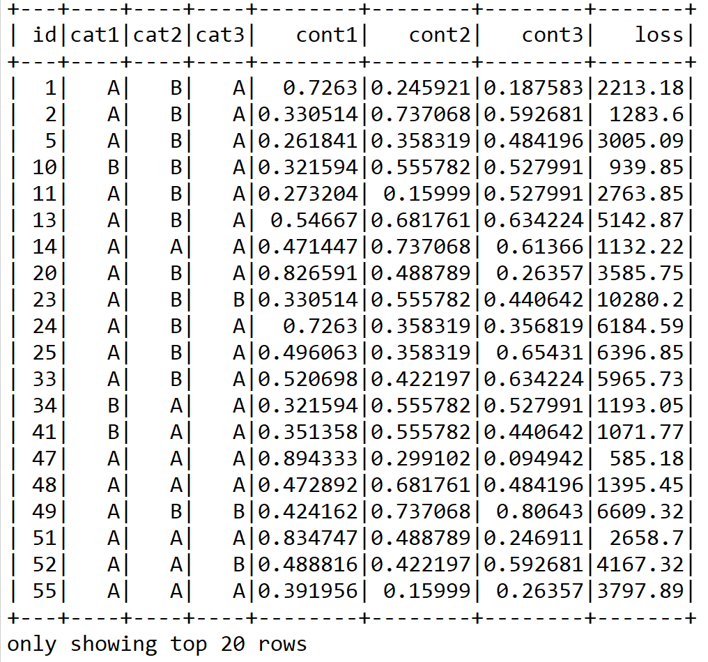
The preceding number is pretty high for training an ML model. Alright, now let's see a snapshot of the dataset using the show() method but with only some selected columns so that it makes more sense. Feel free to use df.show() to see all columns:
df.select("id", "cat1", "cat2", "cat3", "cont1", "cont2", "cont3", "loss").show()
>>> 
Nevertheless, if you look at all the rows using df.show(), you will see some categorical columns containing too many categories. To be more specific, category columns cat109 to cat116 contain too many categories, as follows:
df.select("cat109", "cat110", "cat112", "cat113", "cat116").show()
>>> 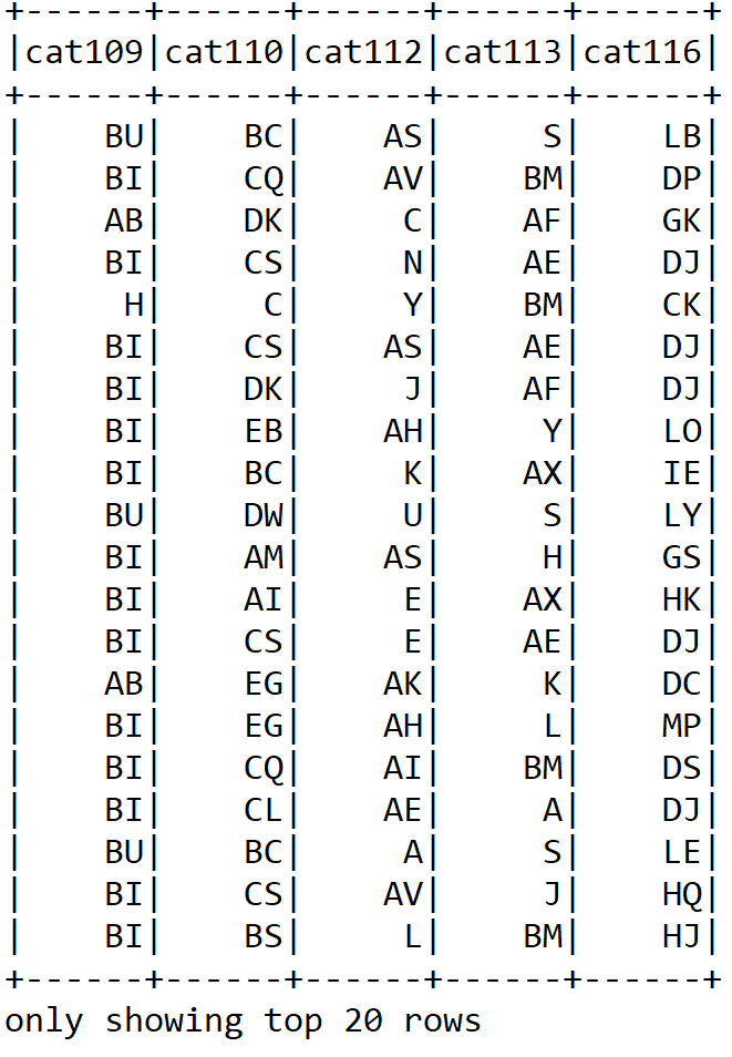
In later stages, it would be worth dropping these columns to remove the skewness in the dataset. It is to be noted that in statistics, skewnessis a measure of the asymmetry of the probability distribution of a real-valued random variable with respect to the mean.
Now that we have seen a snapshot of the dataset, it is worth seeing some other statistics such as average claim or loss, minimum, maximum loss, and many more, using Spark SQL. But before that, let's rename the last column from loss to label since the ML model will complain about it. Even after using the setLabelCol on the regression model, it still looks for a column called label. This results in a disgusting error saying org.apache.spark.sql.AnalysisException: cannot resolve 'label' given input columns:
val newDF = df.withColumnRenamed("loss", "label") Now, since we want to execute an SQL query, we need to create a temporary view so that the operation can be performed in-memory:
newDF.createOrReplaceTempView("insurance") Now let's average the damage claimed by the clients:
spark.sql("SELECT avg(insurance.label) as AVG_LOSS FROM insurance").show()
>>>
+------------------+
| AVG_LOSS |
+------------------+
|3037.3376856699924|
+------------------+
Similarly, let's see the lowest claim made so far:
spark.sql("SELECT min(insurance.label) as MIN_LOSS FROM insurance").show()
>>>
+--------+
|MIN_LOSS|
+--------+
| 0.67|
+--------+
And let's see the highest claim made so far:
spark.sql("SELECT max(insurance.label) as MAX_LOSS FROM insurance").show()
>>>
+---------+
| MAX_LOSS|
+---------+
|121012.25|
+---------+
Since Scala or Java does not come with a handy visualization library, I could not something else but now let's focus on the data preprocessing before we prepare our training set.
Now that we have looked at some data properties, the next task is to do some preprocessing, such as cleaning, before getting the training set. For this part, use the Preprocessing.scala file. For this part, the following imports are required:
import org.apache.spark.ml.feature.{ StringIndexer, StringIndexerModel}
import org.apache.spark.ml.feature.VectorAssembler
Then we load both the training and the test set as shown in the following code:
var trainSample = 1.0
var testSample = 1.0
val train = "data/insurance_train.csv"
val test = "data/insurance_test.csv"
val spark = SparkSessionCreate.createSession()
import spark.implicits._
println("Reading data from " + train + " file")

    val trainInput = spark.read
        .option("header", "true")
        .option("inferSchema", "true")
        .format("com.databricks.spark.csv")
        .load(train)
        .cache

    val testInput = spark.read
        .option("header", "true")
        .option("inferSchema", "true")
        .format("com.databricks.spark.csv")
        .load(test)
        .cache
The next task is to prepare the training and test set for our ML model to be learned. In the preceding DataFrame out of the training dataset, we renamed the loss to label. Then the content of train.csv was split into training and (cross) validation data, 75% and 25%, respectively.
The content of test.csv is used for evaluating the ML model. Both original DataFrames are also sampled, which is particularly useful for running fast executions on your local machine:
println("Preparing data for training model")
var data = trainInput.withColumnRenamed("loss", "label").sample(false, trainSample)
We also should do null checking. Here, I have used a naïve approach. The thing is that if the training DataFrame contains any null values, we completely drop those rows. This makes sense since a few rows out of 188,318 do no harm. However, feel free to adopt another approach such as null value imputation:
var DF = data.na.drop()
if (data == DF)
  println("No null values in the DataFrame")
else{
  println("Null values exist in the DataFrame")
  data = DF
}
val seed = 12345L
val splits = data.randomSplit(Array(0.75, 0.25), seed)
val (trainingData, validationData) = (splits(0), splits(1))
Then we cache both the sets for faster in-memory access:
trainingData.cache
validationData.cache
Additionally, we should perform the sampling of the test set that will be required in the evaluation step:
val testData = testInput.sample(false, testSample).cache Since the training set contains both the numerical and categorical values, we need to identify and treat them separately. First, let's identify only the categorical column:
def isCateg(c: String): Boolean = c.startsWith("cat")
def categNewCol(c: String): String = if (isCateg(c)) s"idx_${c}" else c
Then, the following method is used to remove categorical columns with too many categories, which we already discussed in the preceding section:
def removeTooManyCategs(c: String): Boolean = !(c matches "cat(109$|110$|112$|113$|116$)")Now the following method is used to select only feature columns. So essentially, we should remove the ID (since the ID is just the identification number of the clients, it does not carry any non-trivial information) and the label column:
def onlyFeatureCols(c: String): Boolean = !(c matches "id|label") Well, so far we have treated some bad columns that are either trivial or not needed at all. Now the next task is to construct the definitive set of feature columns:
val featureCols = trainingData.columns
    .filter(removeTooManyCategs)
    .filter(onlyFeatureCols)
    .map(categNewCol)
Note
StringIndexer encodes a given string column of labels to a column of label indices. If the input column is numeric in nature, we cast it to string using the StringIndexer and index the string values. When downstream pipeline components such as Estimator or Transformer make use of this string-indexed label, you must set the input column of the component to this string-indexed column name. In many cases, you can set the input column with setInputCol.
Now we need to use the StringIndexer() for categorical columns:
val stringIndexerStages = trainingData.columns.filter(isCateg)
      .map(c => new StringIndexer()
      .setInputCol(c)
      .setOutputCol(categNewCol(c))
      .fit(trainInput.select(c).union(testInput.select(c))))
Note that this is not an efficient approach. An alternative approach would be using a OneHotEncoder estimator.
Note
OneHotEncoder maps a column of label indices to a column of binary vectors, with a single one-value at most. This encoding permits algorithms that expect continuous features, such as logistic regression, to utilize categorical features.
Now let's use the VectorAssembler() to transform a given list of columns into a single vector column:
val assembler = new VectorAssembler()
    .setInputCols(featureCols)
    .setOutputCol("features")
Note
VectorAssembler is a transformer. It combines a given list of columns into a single vector column. It is useful for combining the raw features and features generated by different feature transformers into one feature vector, in order to train ML models such as logistic regression and decision trees.
That's all we need before we start training the regression models. First, we start training the LR model and evaluate the performance.
As you have already seen, the loss to be predicted contains continuous values, that is, it will be a regression task. So in using regression analysis here, the goal is to predict a continuous target variable, whereas another area called classification predicts a label from a finite set.
Logistic regression (LR) belongs to the family of regression algorithms. The goal of regression is to find relationships and dependencies between variables. It models the relationship between a continuous scalar dependent variable y (that is, label or target) and one or more (a D-dimensional vector) explanatory variable (also independent variables, input variables, features, observed data, observations, attributes, dimensions, and data points) denoted as x using a linear function:

Figure 9: A regression graph separates data points (in red dots) and the blue line is regression
LR models the relationship between a dependent variable y, which involves a linear combination of interdependent variables xi. The letters A and B represent constants that describe the y axis intercept and the slope of the line respectively:
y = A+Bx
Figure 9, Regression graph separates data points (in red dots) and the blue line is regression shows an example of simple LR with one independent variable—that is, a set of data points and a best fit line, which is the result of the regression analysis itself. It can be observed that the line does not actually pass through all of the points.
The distance between any data points (measured) and the line (predicted) is called the regression error. Smaller errors contribute to more accurate results in predicting unknown values. When the errors are reduced to their smallest levels possible, the line of best fit is created for the final regression error. Note that there are no single metrics in terms of regression errors; there are several as follows:
- Mean Squared Error (MSE): It is a measure of how close a fitted line is to data points. The smaller the MSE, the closer the fit is to the data.
- Root Mean Squared Error (RMSE): It is the square root of the MSE but probably the most easily interpreted statistic, since it has the same units as the quantity plotted on the vertical axis.
- R-squared: R-squared is a statistical measure of how close the data is to the fitted regression line. R-squared is always between 0 and 100%. The higher the R-squared, the better the model fits your data.
- Mean Absolute Error (MAE): MAE measures the average magnitude of the errors in a set of predictions without considering their direction. It's the average over the test sample of the absolute differences between prediction and actual observation where all individual differences have equal weight.
- Explained variance: In statistics, explained variation measures the proportion to which a mathematical model accounts for the variation of a given dataset.
In this sub-section, we will develop a predictive analytics model for predicting accidental loss against the severity claim by clients. We start with importing required libraries:
import org.apache.spark.ml.regression.{LinearRegression, LinearRegressionModel}
import org.apache.spark.ml.{ Pipeline, PipelineModel }
import org.apache.spark.ml.evaluation.RegressionEvaluator
import org.apache.spark.ml.tuning.ParamGridBuilder
import org.apache.spark.ml.tuning.CrossValidator
import org.apache.spark.sql._
import org.apache.spark.sql.functions._
import org.apache.spark.mllib.evaluation.RegressionMetrics
Then we create an active Spark session as the entry point to the application. In addition, importing implicits__ required for implicit conversions like converting RDDs to DataFrames.
val spark = SparkSessionCreate.createSession()
import spark.implicits._
Then we define some hyperparameters, such as the number of folds for cross-validation, the number of maximum iterations, the value of the regression parameter, the value of tolerance, and elastic network parameters, as follows:
val numFolds = 10
val MaxIter: Seq[Int] = Seq(1000)
val RegParam: Seq[Double] = Seq(0.001)
val Tol: Seq[Double] = Seq(1e-6)
val ElasticNetParam: Seq[Double] = Seq(0.001)
Well, now we create an LR estimator:
val model = new LinearRegression()
        .setFeaturesCol("features")
        .setLabelCol("label")
Now let's build a pipeline estimator by chaining the transformer and the LR estimator:
println("Building ML pipeline")
val pipeline = new Pipeline()
         .setStages((Preproessing.stringIndexerStages
         :+ Preproessing.assembler) :+ model)
Note
Spark ML pipelines have the following components:
- DataFrame: Used as the central data store where all the original data and intermediate results are stored.
- Transformer: A transformer transforms one DataFrame into another by adding additional feature columns. Transformers are stateless, meaning that they don't have any internal memory and behave exactly the same each time they are used.
- Estimator: An estimator is some sort of ML model. In contrast to a transformer, an estimator contains an internal state representation and is highly dependent on the history of the data that it has already seen.
- Pipeline: Chains the preceding components, DataFrame, Transformer, and Estimator together.
- Parameter: ML algorithms have many knobs to tweak. These are called hyperparameters, and the values learned by a ML algorithm to fit data are called parameters.
Before we start performing the cross-validation, we need to have a paramgrid. So let's start creating the paramgrid by specifying the number of maximum iterations, the value of the regression parameter, the value of tolerance, and Elastic network parameters as follows:
val paramGrid = new ParamGridBuilder()
      .addGrid(model.maxIter, MaxIter)
      .addGrid(model.regParam, RegParam)
      .addGrid(model.tol, Tol)
      .addGrid(model.elasticNetParam, ElasticNetParam)
      .build()
Now, for a better and stable performance, let's prepare the K-fold cross-validation and grid search as a part of model tuning. As you can probably guess, I am going to perform 10-fold cross-validation. Feel free to adjust the number of folds based on your settings and dataset:
println("Preparing K-fold Cross Validation and Grid Search: Model tuning")
val cv = new CrossValidator()
      .setEstimator(pipeline)
      .setEvaluator(new RegressionEvaluator)
      .setEstimatorParamMaps(paramGrid)
      .setNumFolds(numFolds)
Fantastic - we have created the cross-validation estimator. Now it's time to train the LR model:
println("Training model with Linear Regression algorithm")
val cvModel = cv.fit(Preproessing.trainingData)
Now that we have the fitted model, that means it is now capable of making predictions. So let's start evaluating the model on the train and validation set and calculating RMSE, MSE, MAE, R-squared, and many more:
println("Evaluating model on train and validation set and calculating RMSE")
val trainPredictionsAndLabels = cvModel.transform(Preproessing.trainingData)
                .select("label", "prediction")
                .map { case Row(label: Double, prediction: Double)
                => (label, prediction) }.rdd

val validPredictionsAndLabels = cvModel.transform(Preproessing.validationData)
                                .select("label", "prediction")
                                .map { case Row(label: Double, prediction: Double)
                                => (label, prediction) }.rdd

val trainRegressionMetrics = new RegressionMetrics(trainPredictionsAndLabels)
val validRegressionMetrics = new RegressionMetrics(validPredictionsAndLabels)
Great! We have managed to compute the raw prediction on the train and the test set. Let's hunt for the best model:
val bestModel = cvModel.bestModel.asInstanceOf[PipelineModel] Once we have the best fitted and cross-validated model, we can expect good prediction accuracy. Now let's observe the results on the train and the validation set:
val results = "n=====================================================================n" + s"Param trainSample: ${Preproessing.trainSample}n" +
      s"Param testSample: ${Preproessing.testSample}n" +
      s"TrainingData count: ${Preproessing.trainingData.count}n" +
      s"ValidationData count: ${Preproessing.validationData.count}n" +
      s"TestData count: ${Preproessing.testData.count}n" +      "=====================================================================n" +   s"Param maxIter = ${MaxIter.mkString(",")}n" +
      s"Param numFolds = ${numFolds}n" +      "=====================================================================n" +   s"Training data MSE = ${trainRegressionMetrics.meanSquaredError}n" +
      s"Training data RMSE = ${trainRegressionMetrics.rootMeanSquaredError}n" +
      s"Training data R-squared = ${trainRegressionMetrics.r2}n" +
      s"Training data MAE = ${trainRegressionMetrics.meanAbsoluteError}n" +
      s"Training data Explained variance = ${trainRegressionMetrics.explainedVariance}n" +      "=====================================================================n" +   s"Validation data MSE = ${validRegressionMetrics.meanSquaredError}n" +
      s"Validation data RMSE = ${validRegressionMetrics.rootMeanSquaredError}n" +
      s"Validation data R-squared = ${validRegressionMetrics.r2}n" +
      s"Validation data MAE = ${validRegressionMetrics.meanAbsoluteError}n" +
      s"Validation data Explained variance = ${validRegressionMetrics.explainedVariance}n" +
      s"CV params explained: ${cvModel.explainParams}n" +
      s"LR params explained: ${bestModel.stages.last.asInstanceOf[LinearRegressionModel].explainParams}n" +      "=====================================================================n"
Now, we print the preceding results as follows:
println(results)
>>>
Building Machine Learning pipeline
Reading data from data/insurance_train.csv file
Null values exist in the DataFrame
Training model with Linear Regression algorithm
=====================================================================
Param trainSample: 1.0
Param testSample: 1.0
TrainingData count: 141194
ValidationData count: 47124
TestData count: 125546
=====================================================================
Param maxIter = 1000
Param numFolds = 10
=====================================================================
Training data MSE = 4460667.3666198505
Training data RMSE = 2112.0292059107164
Training data R-squared = -0.1514435541595276
Training data MAE = 1356.9375609756164
Training data Explained variance = 8336528.638733305
=====================================================================
Validation data MSE = 4839128.978963534
Validation data RMSE = 2199.802031766389
Validation data R-squared = -0.24922962724089603
Validation data MAE = 1356.419484419514
Validation data Explained variance = 8724661.329105612
CV params explained: estimator: estimator for selection (current: pipeline_d5024480c670)
estimatorParamMaps: param maps for the estimator (current: [Lorg.apache.spark.ml.param.ParamMap;@2f0c9855)
evaluator: evaluator used to select hyper-parameters that maximize the validated metric (current: regEval_00c707fcaa06)
numFolds: number of folds for cross validation (>= 2) (default: 3, current: 10)
seed: random seed (default: -1191137437)
LR params explained: aggregationDepth: suggested depth for treeAggregate (>= 2) (default: 2)
elasticNetParam: the ElasticNet mixing parameter, in range [0, 1]. For alpha = 0, the penalty is an L2 penalty. For alpha = 1, it is an L1 penalty (default: 0.0, current: 0.001)
featuresCol: features column name (default: features, current: features)
fitIntercept: whether to fit an intercept term (default: true)
labelCol: label column name (default: label, current: label)
maxIter: maximum number of iterations (>= 0) (default: 100, current: 1000)
predictionCol: prediction column name (default: prediction)
regParam: regularization parameter (>= 0) (default: 0.0, current: 0.001)
solver: the solver algorithm for optimization. If this is not set or empty, default value is 'auto' (default: auto)
standardization: whether to standardize the training features before fitting the model (default: true)
tol: the convergence tolerance for iterative algorithms (>= 0) (default: 1.0E-6, current: 1.0E-6)
weightCol: weight column name. If this is not set or empty, we treat all instance weights as 1.0 (undefined)
=====================================================================
So our predictive model shows an MAE of about 1356.419484419514 for both the training and test set. However, the MAE is much lower on the Kaggle public and private leaderboard (go to: https://www.kaggle.com/c/allstate-claims-severity/leaderboard) with an MAE of 1096.92532 and 1109.70772 respectively.
Wait! We are not done yet. We still need to make a prediction on the test set:
println("Run prediction on the test set")
cvModel.transform(Preproessing.testData)
      .select("id", "prediction")
      .withColumnRenamed("prediction", "loss")
      .coalesce(1) // to get all the predictions in a single csv file
      .write.format("com.databricks.spark.csv")
      .option("header", "true")
      .save("output/result_LR.csv")
The preceding code should generate a CSV file named result_LR.csv. If we open the file, we should observe the loss against each ID, that is, claim. We will see the contents for both LR, RF, and GBT at the end of this chapter. Nevertheless, it is always a good idea to stop the Spark session by invoking the spark.stop() method.
An ensemble method is a learning algorithm that creates a model that is composed of a set of other base models. Spark ML supports two major ensemble algorithms called GBT and random forest based on decision trees. We will now see if we can improve the prediction accuracy by reducing the MAE error significantly using GBT.
In order to minimize a loss function, Gradient Boosting Trees (GBTs) iteratively train many decision trees. On each iteration, the algorithm uses the current ensemble to predict the label of each training instance.
Then the raw predictions are compared with the true labels. Thus, in the next iteration, the decision tree will help correct previous mistakes if the dataset is re-labeled to put more emphasis on training instances with poor predictions.
Since we are talking about regression, it would be more meaningful to discuss the regression strength of GBTs and its losses computation. Suppose we have the following settings:
- N data instances
- yi = label of instance i
- xi = features of instance i
Then the F(xi) function is the model's predicted label; for instance, it tries to minimize the error, that is, loss:

Now, similar to decision trees, GBTs also:
- Handle categorical features (and of course numerical features too)
- Extend to the multiclass classification setting
- Perform both the binary classification and regression (multiclass classification is not yet supported)
- Do not require feature scaling
- Capture non-linearity and feature interactions, which are greatly missing in LR, such as linear models
Note
Validation while training: Gradient boosting can overfit, especially when you have trained your model with more trees. In order to prevent this issue, it is useful to validate while carrying out the training.
Since we have already prepared our dataset, we can directly jump into implementing a GBT-based predictive model for predicting insurance severity claims. Let's start with importing the necessary packages and libraries:
import org.apache.spark.ml.regression.{GBTRegressor, GBTRegressionModel}
import org.apache.spark.ml.{Pipeline, PipelineModel}
import org.apache.spark.ml.evaluation.RegressionEvaluator
import org.apache.spark.ml.tuning.ParamGridBuilder
import org.apache.spark.ml.tuning.CrossValidator
import org.apache.spark.sql._
import org.apache.spark.sql.functions._
import org.apache.spark.mllib.evaluation.RegressionMetrics
Now let's define and initialize the hyperparameters needed to train the GBTs, such as the number of trees, number of max bins, number of folds to be used during cross-validation, number of maximum iterations to iterate the training, and finally max tree depth:
val NumTrees = Seq(5, 10, 15)
val MaxBins = Seq(5, 7, 9)
val numFolds = 10
val MaxIter: Seq[Int] = Seq(10)
val MaxDepth: Seq[Int] = Seq(10)
Then, again we instantiate a Spark session and implicits as follows:
val spark = SparkSessionCreate.createSession()
import spark.implicits._
Now that we care an estimator algorithm, that is, GBT:
val model = new GBTRegressor()
                .setFeaturesCol("features")
                .setLabelCol("label")
Now, we build the pipeline by chaining the transformations and predictor together as follows:
val pipeline = new Pipeline().setStages((Preproessing.stringIndexerStages :+ Preproessing.assembler) :+ model) Before we start performing the cross-validation, we need to have a paramgrid. So let's start creating the paramgrid by specifying the number of maximum iteration, max tree depth, and max bins as follows:
val paramGrid = new ParamGridBuilder()
      .addGrid(model.maxIter, MaxIter)
      .addGrid(model.maxDepth, MaxDepth)
      .addGrid(model.maxBins, MaxBins)
      .build()
Now, for a better and stable performance, let's prepare the K-fold cross-validation and grid search as a part of model tuning. As you can guess, I am going to perform 10-fold cross-validation. Feel free to adjust the number of folds based on you settings and dataset:
println("Preparing K-fold Cross Validation and Grid Search")
val cv = new CrossValidator()
      .setEstimator(pipeline)
      .setEvaluator(new RegressionEvaluator)
      .setEstimatorParamMaps(paramGrid)
      .setNumFolds(numFolds)
Fantastic, we have created the cross-validation estimator. Now it's time to train the GBT model:
println("Training model with GradientBoostedTrees algorithm ")
val cvModel = cv.fit(Preproessing.trainingData)
Now that we have the fitted model, that means it is now capable of making predictions. So let's start evaluating the model on the train and validation set, and calculating RMSE, MSE, MAE, R-squared, and so on:
println("Evaluating model on train and test data and calculating RMSE")
val trainPredictionsAndLabels = cvModel.transform(Preproessing.trainingData).select("label", "prediction").map { case Row(label: Double, prediction: Double) => (label, prediction) }.rdd

val validPredictionsAndLabels = cvModel.transform(Preproessing.validationData).select("label", "prediction").map { case Row(label: Double, prediction: Double) => (label, prediction) }.rdd

val trainRegressionMetrics = new RegressionMetrics(trainPredictionsAndLabels)
val validRegressionMetrics = new RegressionMetrics(validPredictionsAndLabels)
Great! We have managed to compute the raw prediction on the train and the test set. Let's hunt for the best model:
val bestModel = cvModel.bestModel.asInstanceOf[PipelineModel] As already stated, by using GBT it is possible to measure feature importance so that at a later stage we can decide which features are to be used and which ones are to be dropped from the DataFrame. Let's find the feature importance of the best model we just created previously, for all features in ascending order as follows:
val featureImportances = bestModel.stages.last.asInstanceOf[GBTRegressionModel].featureImportances.toArray
val FI_to_List_sorted = featureImportances.toList.sorted.toArray
Once we have the best fitted and cross-validated model, we can expect good prediction accuracy. Now let's observe the results on the train and the validation set:
val output = "n=====================================================================n" + s"Param trainSample: ${Preproessing.trainSample}n" +
      s"Param testSample: ${Preproessing.testSample}n" +
      s"TrainingData count: ${Preproessing.trainingData.count}n" +
      s"ValidationData count: ${Preproessing.validationData.count}n" +
      s"TestData count: ${Preproessing.testData.count}n" +      "=====================================================================n" +   s"Param maxIter = ${MaxIter.mkString(",")}n" +
      s"Param maxDepth = ${MaxDepth.mkString(",")}n" +
      s"Param numFolds = ${numFolds}n" +      "=====================================================================n" +   s"Training data MSE = ${trainRegressionMetrics.meanSquaredError}n" +
      s"Training data RMSE = ${trainRegressionMetrics.rootMeanSquaredError}n" +
      s"Training data R-squared = ${trainRegressionMetrics.r2}n" +
      s"Training data MAE = ${trainRegressionMetrics.meanAbsoluteError}n" +
      s"Training data Explained variance = ${trainRegressionMetrics.explainedVariance}n" +      "=====================================================================n" +    s"Validation data MSE = ${validRegressionMetrics.meanSquaredError}n" +
      s"Validation data RMSE = ${validRegressionMetrics.rootMeanSquaredError}n" +
      s"Validation data R-squared = ${validRegressionMetrics.r2}n" +
      s"Validation data MAE = ${validRegressionMetrics.meanAbsoluteError}n" +
      s"Validation data Explained variance = ${validRegressionMetrics.explainedVariance}n" +      "=====================================================================n" +   s"CV params explained: ${cvModel.explainParams}n" +
      s"GBT params explained: ${bestModel.stages.last.asInstanceOf[GBTRegressionModel].explainParams}n" + s"GBT features importances:n ${Preproessing.featureCols.zip(FI_to_List_sorted).map(t => s"t${t._1} = ${t._2}").mkString("n")}n" +      "=====================================================================n"
Now, we print the preceding results as follows:
println(results)
 >>>
=====================================================================
Param trainSample: 1.0
Param testSample: 1.0
TrainingData count: 141194
ValidationData count: 47124
TestData count: 125546
=====================================================================
Param maxIter = 10
Param maxDepth = 10
Param numFolds = 10
=====================================================================
Training data MSE = 2711134.460296872
Training data RMSE = 1646.5522950385973
Training data R-squared = 0.4979619968485668
Training data MAE = 1126.582534126603
Training data Explained variance = 8336528.638733303
=====================================================================
Validation data MSE = 4796065.983773314
Validation data RMSE = 2189.9922337244293
Validation data R-squared = 0.13708582379658474
Validation data MAE = 1289.9808960385383
Validation data Explained variance = 8724866.468978886
=====================================================================
CV params explained: estimator: estimator for selection (current: pipeline_9889176c6eda)
estimatorParamMaps: param maps for the estimator (current: [Lorg.apache.spark.ml.param.ParamMap;@87dc030)
evaluator: evaluator used to select hyper-parameters that maximize the validated metric (current: regEval_ceb3437b3ac7)
numFolds: number of folds for cross validation (>= 2) (default: 3, current: 10)
seed: random seed (default: -1191137437)
GBT params explained: cacheNodeIds: If false, the algorithm will pass trees to executors to match instances with nodes. If true, the algorithm will cache node IDs for each instance. Caching can speed up training of deeper trees. (default: false)
checkpointInterval: set checkpoint interval (>= 1) or disable checkpoint (-1). E.g. 10 means that the cache will get checkpointed every 10 iterations (default: 10)
featuresCol: features column name (default: features, current: features)
impurity: Criterion used for information gain calculation (case-insensitive). Supported options: variance (default: variance)
labelCol: label column name (default: label, current: label)
lossType: Loss function which GBT tries to minimize (case-insensitive). Supported options: squared, absolute (default: squared)
maxBins: Max number of bins for discretizing continuous features. Must be >=2 and >= number of categories for any categorical feature. (default: 32)
maxDepth: Maximum depth of the tree. (>= 0) E.g., depth 0 means 1 leaf node; depth 1 means 1 internal node + 2 leaf nodes. (default: 5, current: 10)
maxIter: maximum number of iterations (>= 0) (default: 20, current: 10)
maxMemoryInMB: Maximum memory in MB allocated to histogram aggregation. (default: 256)
minInfoGain: Minimum information gain for a split to be considered at a tree node. (default: 0.0)
minInstancesPerNode: Minimum number of instances each child must have after split. If a split causes the left or right child to have fewer than minInstancesPerNode, the split will be discarded as invalid. Should be >= 1. (default: 1)
predictionCol: prediction column name (default: prediction)
seed: random seed (default: -131597770)
stepSize: Step size (a.k.a. learning rate) in interval (0, 1] for shrinking the contribution of each estimator. (default: 0.1)
subsamplingRate: Fraction of the training data used for learning each decision tree, in range (0, 1]. (default: 1.0)
GBT features importance:
   idx_cat1 = 0.0
   idx_cat2 = 0.0
   idx_cat3 = 0.0
   idx_cat4 = 3.167169394850417E-5
   idx_cat5 = 4.745749854188828E-5
...
   idx_cat111 = 0.018960701085054904
   idx_cat114 = 0.020609596772820878
   idx_cat115 = 0.02281267960792931
   cont1 = 0.023943087007850663
   cont2 = 0.028078353534251005
   ...
   cont13 = 0.06921704925937068
   cont14 = 0.07609111789104464
=====================================================================
So our predictive model shows an MAE of about 1126.582534126603 and 1289.9808960385383 for the training and test sets respectively. The last result is important for understanding the feature importance (the preceding list is abridged to save space but you should receive the full list). Especially, we can see that the first three features are not important at all so we can safely drop them from the DataFrame. We will provide more insight in the next section.
Now finally, let us run the prediction over the test set and generate the predicted loss for each claim from the clients:
println("Run prediction over test dataset")
cvModel.transform(Preproessing.testData)
      .select("id", "prediction")
      .withColumnRenamed("prediction", "loss")
      .coalesce(1)
      .write.format("com.databricks.spark.csv")
      .option("header", "true")
      .save("output/result_GBT.csv")
The preceding code should generate a CSV file named result_GBT.csv. If we open the file, we should observe the loss against each ID, that is, claim. We will see the contents for both LR, RF, and GBT at the end of this chapter. Nevertheless, it is always a good idea to stop the Spark session by invoking the spark.stop() method.
In the previous sections, we did not experience the expected MAE value although we got predictions of the severity loss in each instance. In this section, we will develop a more robust predictive analytics model for the same purpose but use an random forest regressor. However, before diving into its formal implementation, a short overview of the random forest algorithm is needed.
Random Forest is an ensemble learning technique used for solving supervised learning tasks, such as classification and regression. An advantageous feature of Random Forest is that it can overcome the overfitting problem across its training dataset. A forest in Random Forest usually consists of hundreds of thousands of trees. These trees are actually trained on different parts of the same training set.
More technically, an individual tree that grows very deep tends to learn from highly unpredictable patterns. This creates overfitting problems on the training sets. Moreover, low biases make the classifier a low performer even if your dataset quality is good in terms of the features presented. On the other hand, an Random Forest helps to average multiple decision trees together with the goal of reducing the variance to ensure consistency by computing proximities between pairs of cases.
Note
GBT or Random Forest? Although both GBT and Random Forest are ensembles of trees, the training processes are different. There are several practical trade-offs that exist, which often poses the dilemma of which one to choose. However, Random Forest would be the winner in most cases. Here are some justifications:
- GBTs train one tree at a time, but Random Forest can train multiple trees in parallel. So the training time is lower for RF. However, in some special cases, training and using a smaller number of trees with GBTs is easier and quicker.
- RFs are less prone to overfitting in most cases, so it reduces the likelihood of overfitting. In other words, Random Forest reduces variance with more trees, but GBTs reduce bias with more trees.
- Finally, Random Forest can be easier to tune since performance improves monotonically with the number of trees, but GBT performs badly with an increased number of trees.
However, this slightly increases bias and makes it harder to interpret the results. But eventually, the performance of the final model increases dramatically. While using the Random Forest as a classifier, there are some parameter settings:
- If the number of trees is 1, then no bootstrapping is used at all; however, if the number of trees is > 1, then bootstrapping is needed. The supported values are
auto,all,sqrt,log2, andonethird. - The supported numerical values are (0.0-1.0) and [1-n]. However, if
featureSubsetStrategyis chosen asauto, the algorithm chooses the best feature subset strategy automatically. - If the
numTrees == 1, thefeatureSubsetStrategyis set to beall. However, if thenumTrees > 1(that is, forest), thefeatureSubsetStrategyis set to besqrtfor classification. - Moreover, if a real value
nis set in the range of (0, 1.0),n*number_of_featureswill be used. However, if an integer valuenis in the range (1, the number of features) is set, onlynfeatures are used alternatively. - The parameter
categoricalFeaturesInfois a map used for storing arbitrary or of categorical features. An entry (n -> k) indicates that featurenis categorical with I categories indexed from 0: (0, 1,...,k-1). - The impurity criterion is used for information gain calculation. The supported values are
giniandvariancefor classification and regression respectively. - The
maxDepthis the maximum depth of the tree (for example, depth 0 means one leaf node, depth 1 means one internal node plus two leaf nodes). - The
maxBinssignifies the maximum number of bins used for splitting the features, where the suggested value is 100 to get better results. - Finally, the random seed is used for bootstrapping and choosing feature subsets to avoid the random nature of the results.
As already mentioned, since Random Forest is fast and scalable enough for a large-scale dataset, Spark is a suitable technology to implement the RF, and to implement this massive scalability. However, if the proximities are calculated, storage requirements also grow exponentially.
Well, that's enough about RF. Now it's time to get our hands dirty, so let's get started. We begin with importing required libraries:
import org.apache.spark.ml.regression.{RandomForestRegressor, RandomForestRegressionModel}
import org.apache.spark.ml.{ Pipeline, PipelineModel }
import org.apache.spark.ml.evaluation.RegressionEvaluator
import org.apache.spark.ml.tuning.ParamGridBuilder
import org.apache.spark.ml.tuning.CrossValidator
import org.apache.spark.sql._
import org.apache.spark.sql.functions._
import org.apache.spark.mllib.evaluation.RegressionMetrics
Then we create an active Spark session and import implicits:
val spark = SparkSessionCreate.createSession()
import spark.implicits._
Then we define some hyperparameters, such as the number of folds for cross-validation, number of maximum iterations, the value of regression parameters, value of tolerance, and elastic network parameters, as follows:
val NumTrees = Seq(5,10,15)
val MaxBins = Seq(23,27,30)
val numFolds = 10
val MaxIter: Seq[Int] = Seq(20)
val MaxDepth: Seq[Int] = Seq(20)
Note that for an Random Forest based on a decision tree, we require maxBins to be at least as large as the number of values in each categorical feature. In our dataset, we have 110 categorical features with 23 distinct values. Considering this, we have to set MaxBins to at least 23. Nevertheless, feel free to play with the previous parameters too. Alright, now it's time to create an LR estimator:
val model = new RandomForestRegressor().setFeaturesCol("features").setLabelCol("label")Now let's build a pipeline estimator by chaining the transformer and the LR estimator:
println("Building ML pipeline")
val pipeline = new Pipeline().setStages((Preproessing.stringIndexerStages :+ Preproessing.assembler) :+ model)
Before we start performing the cross-validation, we need to have a paramgrid. So let's start creating the paramgrid by specifying the number of trees, a number for maximum tree depth, and the number of maximum bins parameters, as follows:
val paramGrid = new ParamGridBuilder()
      .addGrid(model.numTrees, NumTrees)
      .addGrid(model.maxDepth, MaxDepth)
      .addGrid(model.maxBins, MaxBins)
      .build()
Now, for better and stable performance, let's prepare the K-fold cross-validation and grid search as a part of model tuning. As you can probably guess, I am going to perform 10-fold cross-validation. Feel free to adjust the number of folds based on your settings and dataset:
println("Preparing K-fold Cross Validation and Grid Search: Model tuning")
val cv = new CrossValidator()
      .setEstimator(pipeline)
      .setEvaluator(new RegressionEvaluator)
      .setEstimatorParamMaps(paramGrid)
      .setNumFolds(numFolds)
Fantastic, we have created the cross-validation estimator. Now it's time to train the LR model:
println("Training model with Random Forest algorithm")
val cvModel = cv.fit(Preproessing.trainingData)
Now that we have the fitted model, that means it is now capable of making predictions. So let's start evaluating the model on the train and validation set, and calculating RMSE, MSE, MAE, R-squared, and many more:
println("Evaluating model on train and validation set and calculating RMSE")
val trainPredictionsAndLabels = cvModel.transform(Preproessing.trainingData).select("label", "prediction").map { case Row(label: Double, prediction: Double) => (label, prediction) }.rdd

val validPredictionsAndLabels = cvModel.transform(Preproessing.validationData).select("label", "prediction").map { case Row(label: Double, prediction: Double) => (label, prediction) }.rdd

val trainRegressionMetrics = new RegressionMetrics(trainPredictionsAndLabels)
val validRegressionMetrics = new RegressionMetrics(validPredictionsAndLabels)
Great! We have managed to compute the raw prediction on the train and the test set. Let's hunt for the best model:
val bestModel = cvModel.bestModel.asInstanceOf[PipelineModel]
As already stated, by using RF, it is possible to measure the feature importance so that at a later stage, we can decide which features should be used and which ones are to be dropped from the DataFrame. Let's find the feature importance from the best model we just created for all features in ascending order, as follows:
val featureImportances = bestModel.stages.last.asInstanceOf[RandomForestRegressionModel].featureImportances.toArray
val FI_to_List_sorted = featureImportances.toList.sorted.toArray
Once we have the best fitted and cross-validated model, we can expect a good prediction accuracy. Now let's observe the results on the train and the validation set:
val output = "n=====================================================================n" + s"Param trainSample: ${Preproessing.trainSample}n" +
      s"Param testSample: ${Preproessing.testSample}n" +
      s"TrainingData count: ${Preproessing.trainingData.count}n" +
      s"ValidationData count: ${Preproessing.validationData.count}n" +
      s"TestData count: ${Preproessing.testData.count}n" +      "=====================================================================n" +   s"Param maxIter = ${MaxIter.mkString(",")}n" +
      s"Param maxDepth = ${MaxDepth.mkString(",")}n" +
      s"Param numFolds = ${numFolds}n" +      "=====================================================================n" +   s"Training data MSE = ${trainRegressionMetrics.meanSquaredError}n" +
      s"Training data RMSE = ${trainRegressionMetrics.rootMeanSquaredError}n" +
      s"Training data R-squared = ${trainRegressionMetrics.r2}n" +
      s"Training data MAE = ${trainRegressionMetrics.meanAbsoluteError}n" +
      s"Training data Explained variance = ${trainRegressionMetrics.explainedVariance}n" +      "=====================================================================n" +   s"Validation data MSE = ${validRegressionMetrics.meanSquaredError}n" +
      s"Validation data RMSE = ${validRegressionMetrics.rootMeanSquaredError}n" +
      s"Validation data R-squared = ${validRegressionMetrics.r2}n" +
      s"Validation data MAE = ${validRegressionMetrics.meanAbsoluteError}n" +
      s"Validation data Explained variance =
${validRegressionMetrics.explainedVariance}n" +      "=====================================================================n" +   s"CV params explained: ${cvModel.explainParams}n" +
      s"RF params explained: ${bestModel.stages.last.asInstanceOf[RandomForestRegressionModel].explainParams}n" +
      s"RF features importances:n ${Preproessing.featureCols.zip(FI_to_List_sorted).map(t => s"t${t._1} = ${t._2}").mkString("n")}n" +      "=====================================================================n"
Now, we print the preceding results as follows:
println(results) >>>Param trainSample: 1.0 Param testSample: 1.0 TrainingData count: 141194 ValidationData count: 47124 TestData count: 125546 Param maxIter = 20 Param maxDepth = 20 Param numFolds = 10 Training data MSE = 1340574.3409399686 Training data RMSE = 1157.8317412042081 Training data R-squared = 0.7642745310548124 Training data MAE = 809.5917285994619 Training data Explained variance = 8337897.224852404 Validation data MSE = 4312608.024875177 Validation data RMSE = 2076.6819749001475 Validation data R-squared = 0.1369507149716651" Validation data MAE = 1273.0714382935894 Validation data Explained variance = 8737233.110450774
So our predictive model shows an MAE of about 809.5917285994619 and 1273.0714382935894 for the training and test set respectively. The last result is important for understanding the feature importance (the preceding list is abridged to save space but you should receive the full list).
I have drawn both the categorical and continuous features, and their respective importance in Python, so I will not show the code here but only the graph. Let's see the categorical features showing feature importance as well as the corresponding feature number:

Figure 11: Random Forest categorical feature importance
From the preceding graph, it is clear that categorical features cat20, cat64, cat47, and cat69 are less important. Therefore, it would make sense to drop these features and retrain the Random Forest model to observe better performance.
Now let's see how the continuous features are correlated and contribute to the loss column. From the following figure, we can see that all continuous features are positively correlated with the loss column. This also signifies that these continuous features are not that important compared to the categorical ones we have seen in the preceding figure:

Figure 12: Correlations between the continuous features and the label
What we can learn from these two analyses is that we can naively drop some unimportant columns and train the Random Forest model to observe if there is any reduction in the MAE value for both the training and validation set. Finally, let's make a prediction on the test set:
println("Run prediction on the test set")
cvModel.transform(Preproessing.testData)
      .select("id", "prediction")
      .withColumnRenamed("prediction", "loss")
      .coalesce(1) // to get all the predictions in a single csv file
      .write.format("com.databricks.spark.csv")
      .option("header", "true")
      .save("output/result_RF.csv")
Also, similar to LR, you can stop the Spark session by invoking the stop() method. Now the generated result_RF.csv file should contain the loss against each ID, that is, claim.
You have already seen that the LR model is much easier to train for a small training dataset. However, we haven't experienced better accuracy compared to GBT and Random Forest models. However, the simplicity of the LR model is a very good starting point. On the other hand, we already argued that Random Forest would be the winner over GBT for several reasons, of course. Let's see the results in a table:

Now let's see how the predictions went for each model for 20 accidents or damage claims:

Figure 13: Loss prediction by i) LR, ii) GBT, and iii) Random Forest models
Therefore, based on table 2, it is clear that we should go with the Random Forest regressor to not only predict the insurance claim loss but also its production. Now we will see a quick overview of how to take our best model, that is, an Random Forest regressor into production. The idea is, as a data scientist, you may have produced an ML model and handed it over to an engineering team in your company for deployment in a production-ready environment.
Here, I provide a naïve approach, though IT companies must have their own way to deploy the models. Nevertheless, there will be a dedicated section at the end of this topic. This scenario can easily become a reality by using model persistence—the ability to save and load models that come with Spark. Using Spark, you can either:
- Save and load a single model
- Save and load a full pipeline
A single model is pretty simple, but less effective and mainly works on Spark MLlib-based model persistence. Since we are more interested in saving the best model, that is, the Random Forest regressor model, at first we will fit an Random Forest regressor using Scala, save it, and then load the same model back using Scala:
// Estimator algorithm
val model = new RandomForestRegressor()
                    .setFeaturesCol("features")
                    .setLabelCol("label")
                    .setImpurity("gini")
                    .setMaxBins(20)
                    .setMaxDepth(20)
                    .setNumTrees(50)
fittedModel = rf.fit(trainingData)
We can now simply call the write.overwrite().save() method to save this model to local storage, HDFS, or S3, and the load method to load it right back for future use:
fittedModel.write.overwrite().save("model/RF_model")
val sameModel = CrossValidatorModel.load("model/RF_model")
Now the thing that we need to know is how to use the restored model for making predictions. Here's the answer:
sameModel.transform(Preproessing.testData)
    .select("id", "prediction")
    .withColumnRenamed("prediction", "loss")
    .coalesce(1)
    .write.format("com.databricks.spark.csv")
    .option("header", "true")
.save("output/result_RF_reuse.csv") 
Figure 14: Spark model deployment for production
So far, we have only looked at saving and loading a single ML model but not a tuned or stable one. It might even provide you with many wrong predictions. Therefore, now the second approach might be more effective.
The reality is that, in practice, ML workflows consist of many stages, from feature extraction and transformation to model fitting and tuning. Spark ML provides pipelines to help users construct these workflows. Similarly, a pipeline with the cross-validated model can be saved and restored back the same way as we did in the first approach.
We fit the cross-validated model with the training set:
val cvModel = cv.fit(Preproessing.trainingData)
Then we save the workflow/pipeline:
cvModel.write.overwrite().save("model/RF_model") Note that the preceding line of code will save the model in your preferred location with the following directory structure:

Figure 15: Saved model directory structure
//Then we restore the same model back:
val sameCV = CrossValidatorModel.load("model/RF_model")
Now when you try to restore the same model, Spark will automatically pick the best one. Finally, we reuse this model for making a prediction as follows:
sameCV.transform(Preproessing.testData)
      .select("id", "prediction")
      .withColumnRenamed("prediction", "loss")
      .coalesce(1)
      .write.format("com.databricks.spark.csv")
      .option("header", "true")
.save("output/result_RF_reuse.csv") In a production ready environment, we often need to deploy a pretrained models in scale. Especially, if we need to handle a massive amount of data. So our ML model has to face this scalability issue to perform continiously and with faster response. To overcome this issue, one of the main big data paradigms that Spark has brought for us is the introduction of in-memory computing (it supports dis based operation, though) and caching abstraction.
This makes Spark ideal for large-scale data processing and enables the computing nodes to perform multiple operations by accessing the same input data across multiple nodes in a computing cluster or cloud computing infrastructures (example, Amazon AWS, DigitalOcean, Microsoft Azure, or Google Cloud). For doing so, Spark supports four cluster managers (the last one is still experimental, though):
- Standalone: A simple cluster manager included with Spark that makes it easy to set up a cluster.
- Apache Mesos: A general cluster manager that can also run Hadoop MapReduce and service applications.
- Hadoop YARN: The resource manager in Hadoop 2.
- Kubernetes (experimental): In addition to the above, there is experimental support for Kubernetes. Kubernetes is an open-source platform for providing container-centric infrastructure. See more at https://spark.apache.org/docs/latest/cluster-overview.html.
You can upload your input dataset on Hadoop Distributed File System (HDFS) or S3 storage for efficient computing and storing big data cheaply. Then the spark-submit script in Spark’s bin directory is used to launch applications on any of those cluster modes. It can use all of the cluster managers through a uniform interface so you don’t have to configure your application specially for each one.
However, if your code depends on other projects, you will need to package them alongside your application in order to distribute the code to a Spark cluster. To do this, create an assembly jar (also called fat or uber jar) containing your code and its dependencies. Then ship the code where the data resides and execute your Spark jobs. Both the SBT and Maven have assembly plugins that should help you to prepare the jars.
When creating assembly jars, list Spark and Hadoop as dependencies as well. These need not be bundled since they are provided by the cluster manager at runtime. Once you have an assembled jar, you can call the script by passing your jar as follows:
  ./bin/spark-submit \
      --class <main-class> \
      --master <master-url> \
      --deploy-mode <deploy-mode> \
      --conf <key>=<value> \
       ... # other options
       <application-jar> \
       [application-arguments]
In the preceding command, some of the commonly used options are listed down as follows:
--class: The entry point for your application (example,org.apache.spark.examples.SparkPi).--master: The master URL for the cluster (example,spark://23.195.26.187:7077).--deploy-mode: Whether to deploy your driver on the worker nodes (cluster) or locally as an external client.--conf: Arbitrary Spark configuration property in key=value format.application-jar: Path to a bundled jar including your application and all dependencies. The URL must be globally visible inside of your cluster, for instance, anhdfs://path or afile://path that is present on all nodes.application-arguments: Arguments passed to the main method of your main class, if any.
For example, you can run the AllstateClaimsSeverityRandomForestRegressor script on a Spark standalone cluster in client deploy mode as follows:
./bin/spark-submit \
   --class com.packt.ScalaML.InsuranceSeverityClaim.AllstateClaimsSeverityRandomForestRegressor\
   --master spark://207.184.161.138:7077 \
   --executor-memory 20G \
   --total-executor-cores 100 \
   /path/to/examples.jar
For more info see Spark website at https://spark.apache.org/docs/latest/submitting-applications.html. Nevertheless, you can find useful information from online blogs or books. By the way, I discussed this topic in details in one of my recently published books: Md. Rezaul Karim, Sridhar Alla, Scala and Spark for Big Data Analytics, Packt Publishing Ltd. 2017. See more at https://www.packtpub.com/big-data-and-business-intelligence/scala-and-spark-big-data-analytics.
Anyway, we will learn more on deploying ML models in production in upcoming chapters. Therefore, that's all I have to write for this chapter.
In this chapter, we have seen how to develop a predictive model for analyzing insurance severity claims using some of the most widely used regression algorithms. We started with simple LR. Then we saw how we can improve performance using a GBT regressor. Then we experienced improved performance using ensemble techniques, such as the Random Forest regressor. Finally, we looked at performance comparative analysis between these models and chose the best model to deploy for production-ready environment.
In the next chapter, we will look at a new end-to-end project called Analyzing and Predicting Telecommunication Churn. Churn prediction is essential for businesses as it helps you detect customers who are likely to cancel a subscription, product, or service. It also minimizes customer defection. It does so by predicting which customers are more likely to cancel a subscription to a service.
