Download code from GitHub
Spark SQL is at the heart of all applications developed using Spark. In this book, we will explore Spark SQL in great detail, including its usage in various types of applications as well as its internal workings. Developers and architects will appreciate the technical concepts and hands-on sessions presented in each chapter, as they progress through the book.
In this chapter, we will introduce you to the key concepts related to Spark SQL. We will start with SparkSession, the new entry point for Spark SQL in Spark 2.0. Then, we will explore Spark SQL's interfaces RDDs, DataFrames, and Dataset APIs. Later on, we will explain the developer-level details regarding the Catalyst optimizer and Project Tungsten.
Finally, we will introduce an exciting new feature in Spark 2.0 for streaming applications, called Structured Streaming. Specific hands-on exercises (using publicly available Datasets) are presented throughout the chapter, so you can actively follow along as you read through the various sections.
More specifically, the sections in this chapter will cover the following topics along with practice hands-on sessions:
- What is Spark SQL?
- Introducing SparkSession
- Understanding Spark SQL concepts
- Understanding RDDs, DataFrames, and Datasets
- Understanding the Catalyst optimizer
- Understanding Project Tungsten
- Using Spark SQL in continuous applications
- Understanding Structured Streaming internals
Spark SQL is one of the most advanced components of Apache Spark. It has been a part of the core distribution since Spark 1.0 and supports Python, Scala, Java, and R programming APIs. As illustrated in the figure below, Spark SQL components provide the foundation for machine learning applications, streaming applications, graph applications, and many other types of application architectures.

Such applications, typically, use Spark ML pipelines, Structured Streaming, and GraphFrames, which are all based on Spark SQL interfaces (DataFrame/Dataset API). These applications, along with constructs such as SQL, DataFrames, and Datasets API, receive the benefits of the Catalyst optimizer, automatically. This optimizer is also responsible for generating executable query plans based on the lower-level RDD interfaces.
We will explore ML pipelines in more detail in Chapter 6, Using Spark SQL in Machine Learning Applications. GraphFrames will be covered in Chapter 7, Using Spark SQL in Graph Applications. While, we will introduce the key concepts regarding Structured Streaming and the Catalyst optimizer in this chapter, we will get more details about them in Chapter 5, Using Spark SQL in Streaming Applications, and Chapter 11, Tuning Spark SQL Components for Performance.
In Spark 2.0, the DataFrame API has been merged with the Dataset API, thereby unifying data processing capabilities across Spark libraries. This also enables developers to work with a single high-level and type-safe API. However, the Spark software stack does not prevent developers from directly using the low-level RDD interface in their applications. Though the low-level RDD API will continue to be available, a vast majority of developers are expected to (and are recommended to) use the high-level APIs, namely, the Dataset and DataFrame APIs.
Additionally, Spark 2.0 extends Spark SQL capabilities by including a new ANSI SQL parser with support for subqueries and the SQL:2003 standard. More specifically, the subquery support now includes correlated/uncorrelated subqueries, and IN / NOT IN and EXISTS / NOTEXISTS predicates in WHERE / HAVING clauses.
At the core of Spark SQL is the Catalyst optimizer, which leverages Scala's advanced features, such as pattern matching, to provide an extensible query optimizer. DataFrames, Datasets, and SQL queries share the same execution and optimization pipeline; hence, there is no performance of using any one or the other of these constructs (or of using any of the supported programming APIs). The high-level DataFrame-based code written by the developer is converted to Catalyst expressions and then to low-level Java bytecode as it passes through this pipeline.
SparkSession is the entry point into Spark SQL-related functionality and we describe it in more detail in the next section.
In Spark 2.0, SparkSession represents a unified point for manipulating data in Spark. It minimizes the number of different contexts a developer has to use while working with Spark. SparkSession replaces multiple context objects, such as the SparkContext, SQLContext, and HiveContext. These contexts are now encapsulated within the SparkSession object.
In Spark programs, we use the builder design pattern to instantiate a SparkSession object. However, in the REPL environment (that is, in a Spark shell session), the SparkSession is automatically created and made available to you via an instance object called Spark.
At this time, start the Spark shell on your computer to interactively execute the code snippets in this section. As the shell starts up, you will notice a bunch of messages appearing on your screen, as shown in the following figure. You should see messages displaying the availability of a SparkSession object (as Spark), Spark version as 2.2.0, Scala version as 2.11.8, and the Java version as 1.8.x.

The SparkSession object can be used to configure Spark's runtime config properties. For example, the two main resources that Spark and Yarn manage are the CPU the memory. If you want to set the number of cores and the heap size for the Spark executor, then you can do that by setting the spark.executor.cores and the spark.executor.memory properties, respectively. In this example, we set these runtime properties to 2 cores and 4 GB, respectively, as shown:
    scala> spark.conf.set("spark.executor.cores", "2")

    scala> spark.conf.set("spark.executor.memory", "4g")
The SparkSession object can be used to read data from various sources, such as CSV, JSON, JDBC, stream, and so on. In addition, it can be used to execute SQL statements, register User Defined Functions (UDFs), and work with Datasets and DataFrames. The following illustrates some of these basic operations in Spark.
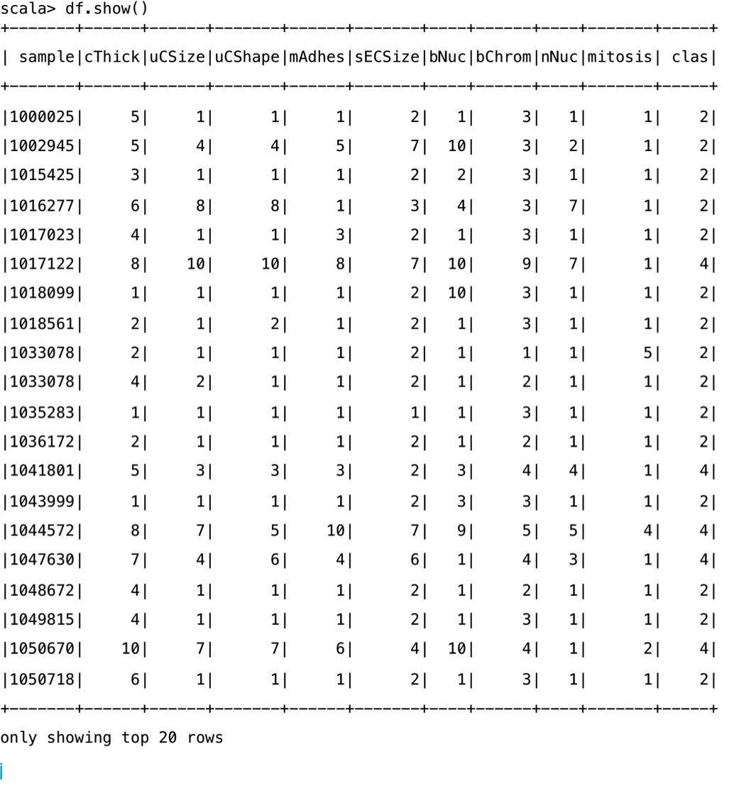
For this example, we use the breast cancer database created by Dr. William H. Wolberg, University of Wisconsin Hospitals, Madison. You can download the original Dataset from https://archive.ics.uci.edu/ml/datasets/Breast+Cancer+Wisconsin+(Original). Each row in the dataset contains the sample number, nine cytological characteristics of breast fine needle aspirates graded 1 to 10, and the class label , benign (2) or malignant (4).
First, we define a schema for the records in our file. The field descriptions are available at the Dataset's download site.
scala> import org.apache.spark.sql.types._

scala> val recordSchema = new StructType().add("sample", "long").add("cThick", "integer").add("uCSize", "integer").add("uCShape", "integer").add("mAdhes", "integer").add("sECSize", "integer").add("bNuc", "integer").add("bChrom", "integer").add("nNuc", "integer").add("mitosis", "integer").add("clas", "integer")
Next, we create a DataFrame from our input CSV file using the schema defined in the preceding step:
val df = spark.read.format("csv").option("header", false).schema(recordSchema).load("file:///Users/aurobindosarkar/Downloads/breast-cancer-wisconsin.data")The newly created DataFrame can be displayed using the show() method:
The DataFrame can be registered as a SQL temporary view using the createOrReplaceTempView() method. This allows applications to run SQL queries using the sql function of the SparkSession object and return the results as a DataFrame.
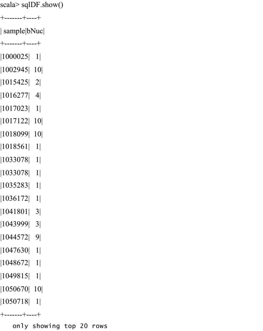
Next, we create a temporary view for the DataFrame and a simple SQL statement against it:
scala> df.createOrReplaceTempView("cancerTable")

scala> val sqlDF = spark.sql("SELECT sample, bNuc from cancerTable")
The contents of results DataFrame are displayed using the show() method:
In the next code snippet, we show you the statements for creating a Spark Dataset using a case class and the toDS() method. Then, we define a UDF to convert the clas column, currently containing 2's and 4's to 0's and 1's respectively. We register the UDF using the SparkSession object and it in a SQL statement:
scala> case class CancerClass(sample: Long, cThick: Int, uCSize: Int, uCShape: Int, mAdhes: Int, sECSize: Int, bNuc: Int, bChrom: Int, nNuc: Int, mitosis: Int, clas: Int)

scala> val cancerDS = spark.sparkContext.textFile("file:///Users/aurobindosarkar/Documents/SparkBook/data/breast-cancer-wisconsin.data").map(_.split(",")).map(attributes => CancerClass(attributes(0).trim.toLong, attributes(1).trim.toInt, attributes(2).trim.toInt, attributes(3).trim.toInt, attributes(4).trim.toInt, attributes(5).trim.toInt, attributes(6).trim.toInt, attributes(7).trim.toInt, attributes(8).trim.toInt, attributes(9).trim.toInt, attributes(10).trim.toInt)).toDS()

scala> def binarize(s: Int): Int = s match {case 2 => 0 case 4 => 1 }

scala> spark.udf.register("udfValueToCategory", (arg: Int) => binarize(arg))

scala> val sqlUDF = spark.sql("SELECT *, udfValueToCategory(clas) from cancerTable")

scala> sqlUDF.show()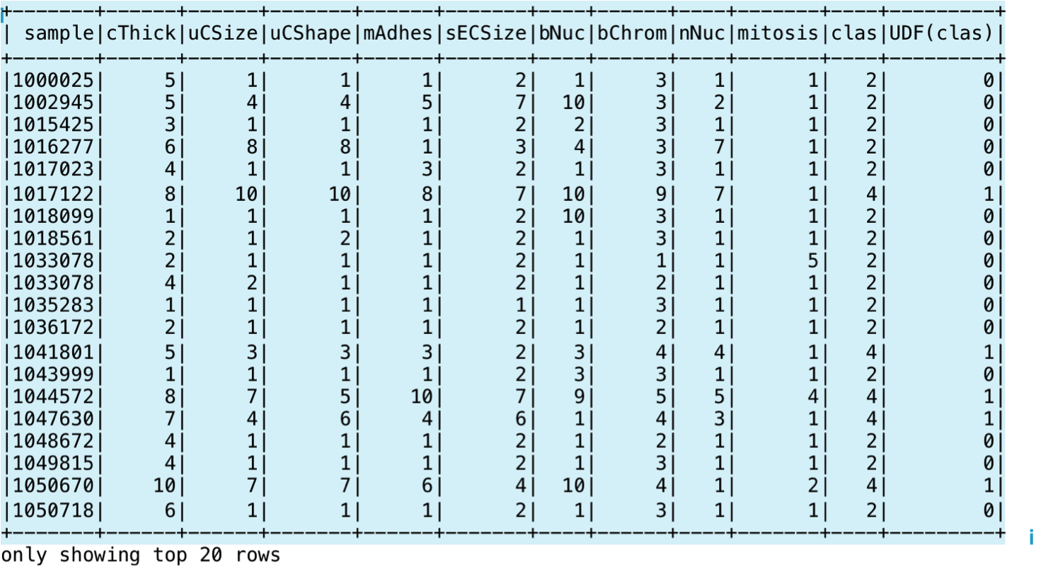
SparkSession exposes methods (via the catalog attribute) of accessing the underlying metadata, such as the available databases and tables, registered UDFs, temporary views, and so on. Additionally, we can also cache tables, drop temporary views, and clear the cache. Some of these statements and corresponding output are shown here:
scala> spark.catalog.currentDatabase

res5: String = default

scala> spark.catalog.isCached("cancerTable")

res6: Boolean = false

scala> spark.catalog.cacheTable("cancerTable")

scala> spark.catalog.isCached("cancerTable")

res8: Boolean = true

scala> spark.catalog.clearCache

scala> spark.catalog.isCached("cancerTable")

res10: Boolean = false

scala> spark.catalog.listDatabases.show()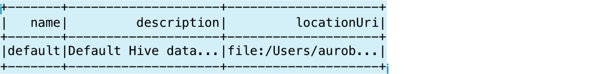
can also use the take method to display a specific number of records in the DataFrame:
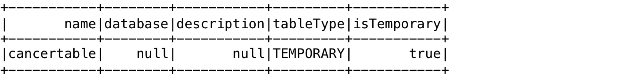
scala> spark.catalog.listDatabases.take(1)
res13: Array[org.apache.spark.sql.catalog.Database] = Array(Database[name='default', description='Default Hive database', path='file:/Users/aurobindosarkar/Downloads/spark-2.2.0-bin-hadoop2.7/spark-warehouse'])

scala> spark.catalog.listTables.show()
We can drop the temp table we created earlier with the following statement:
scala> spark.catalog.dropTempView("cancerTable")

scala> spark.catalog.listTables.show()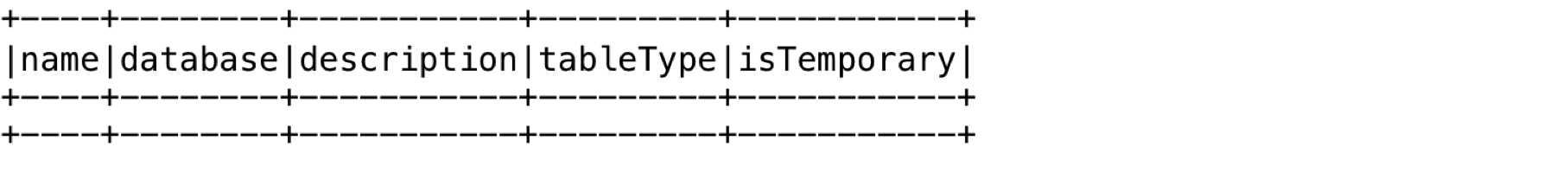
In the next few sections, we will describe RDDs, DataFrames, and Dataset constructs in more detail.
In this section, we will explore concepts related to Resilient Distributed Datasets (RDD), DataFrames, and Datasets, Catalyst Optimizer and Project Tungsten.
RDDs are Spark's primary distributed Dataset abstraction. It is a collection of data that is immutable, distributed, lazily evaluated, type inferred, and cacheable. Prior to execution, the developer code (using higher-level constructs such as SQL, DataFrames, and Dataset APIs) is converted to a DAG of RDDs (ready for execution).
You can create RDDs by parallelizing existing collection of or accessing a Dataset residing in an external storage system, such as the file system or various Hadoop-based data sources. The parallelized collections form a distributed Dataset that enable parallel operations on them.
You can create a RDD from the input file with number of partitions specified, as shown:
scala> val cancerRDD = sc.textFile("file:///Users/aurobindosarkar/Downloads/breast-cancer-wisconsin.data", 4)

scala> cancerRDD.partitions.size
res37: Int = 4
You can implicitly convert the RDD to a DataFrame by importing the spark.implicits package and using the toDF() method:
scala> import spark.implicits._scala>
val cancerDF = cancerRDD.toDF()
To create a DataFrame with a specific schema, we define a Row object for the rows contained in the DataFrame. Additionally, we split the comma-separated data, convert it to a list of fields, and then map it to the Row object. Finally, we use the createDataFrame() to create the DataFrame with a specified schema:
def row(line: List[String]): Row = { Row(line(0).toLong, line(1).toInt, line(2).toInt, line(3).toInt, line(4).toInt, line(5).toInt, line(6).toInt, line(7).toInt, line(8).toInt, line(9).toInt, line(10).toInt) }
val data = cancerRDD.map(_.split(",").to[List]).map(row)
val cancerDF = spark.createDataFrame(data, recordSchema)
Further, we can easily convert the preceding DataFrame to a Dataset using the case class defined earlier:
scala> val cancerDS = cancerDF.as[CancerClass]RDD data is logically divided into a set of partitions; additionally, all input, intermediate, and output data is also represented as partitions. The number of RDD partitions defines the level of data fragmentation. These partitions are also the basic units of parallelism. Spark execution are split into multiple stages, and as each stage operates on one partition at a time, it is very important to tune the number of partitions. Fewer partitions than active stages means your cluster could be under-utilized, while an excessive number of partitions could impact the performance due to higher disk and network I/O.
The programming interface to RDDs support two of operations: transformations and actions. The transformations create a new Dataset from an existing one, while the actions return a value or result of a computation. All transformations are evaluated lazily--the actual execution occurs only when an action is executed to compute a result. The transformations form a lineage graph instead of actually replicating data across multiple machines. This graph-based approach enables an efficient fault tolerance model. For example, if an RDD partition is lost, then it can be recomputed based on the lineage graph.
You can control data persistence (for example, caching) and specify placement preferences for RDD partitions and then use specific operators for manipulating them. By default, Spark persists RDDs in memory, but it can spill them to disk if sufficient RAM isn't available. Caching improves performance by several orders of magnitude; however, it is often memory intensive. Other persistence options storing RDDs to disk and replicating them across the nodes in your cluster. The in-memory storage of persistent RDDs can be in the of deserialized or serialized Java objects. The deserialized option is faster, while the serialized option is more memory-efficient (but slower). Unused RDDs are automatically removed from the cache but, depending on your requirements; if a specific RDD is no longer required, then you can also explicitly release it.
A DataFrame is similar to a table in a relational database, a pandas dataframe, or a data frame in R. It is a distributed collection of that is organized into columns. It the immutable, in-memory, resilient, distributed, and parallel capabilities of RDD, and applies a schema to the data. DataFrames are evaluated lazily. Additionally, they provide a domain-specific language (DSL) for distributed data manipulation.
Conceptually, the DataFrame is an for a collection of generic objects Dataset[Row], where a row is a generic untyped object. This means that syntax errors for DataFrames are caught during the compile stage; however, analysis errors are detected only during runtime.
DataFrames can be constructed from a wide array of sources, such as structured data files, Hive tables, databases, or RDDs. The source data can be read from local filesystems, HDFS, Amazon S3, and RDBMSs. In addition, other popular data formats, such as CSV, JSON, Avro, Parquet, and so on, are also supported. Additionally, you can also create and use custom data sources.
The DataFrame API supports Scala, Java, Python, and R programming APIs. The DataFrames API is declarative, and combined with procedural Spark code, it provides a much tighter integration between the relational and procedural processing in your applications. DataFrames can be manipulated using Spark's procedural API, or using relational APIs (with richer optimizations).
In the early versions of Spark, you had to write arbitrary Java, Python, or Scala functions that operated on RDDs. In this scenario, the functions were executing on opaque Java objects. Hence, the user functions were essentially black boxes executing opaque computations using opaque objects and data types. This approach was very general and such programs had complete control over the execution of every data operation. However, as the engine did not know the code you were executing or nature of the data, it was not possible to optimize these arbitrary Java objects. In addition, it was incumbent on the developers to write efficient programs were dependent on the nature of their specific workloads.
In Spark 2.0, the main benefit of using SQL, DataFrames, and Datasets is that it's easier to program using these high-level programming interfaces while reaping the benefits of improved performance, automatically. You have to write significantly fewer lines of and the programs are automatically optimized and efficient code is generated for you. This results in better performance while significantly reducing the burden on developers. Now, the developer can focus on the "what" rather than the "how" of something that needs to be accomplished.
The Dataset API was first added to Spark 1.6 to provide the benefits of both RDDs and the Spark SQL's optimizer. A Dataset can be constructed from JVM objects and then manipulated using functional transformations such as map, filter, and so on. As the Dataset is a collection of strongly-typed objects specified using a user-defined case class, both syntax errors and analysis errors can be detected at compile time.
The unified Dataset API can be used in both Scala and Java. However, Python does not support the Dataset API yet.
In the following example, we present a few basic DataFrame/Dataset operations. For this purpose, we will use two restaurant listing datasets that are typically used in duplicate records detection and record linkage applications. The two lists, one each from Zagat's and Fodor's restaurant guides, have duplicate records between them. To keep this example simple, we have manually converted the input files to a CSV format. You can download the original dataset from http://www.cs.utexas.edu/users/ml/riddle/data.html.
First, we define a case class for the records in the two files:
scala> case class RestClass(name: String, street: String, city: String, phone: String, cuisine: String)
Next, we create Datasets from the two files:
scala> val rest1DS = spark.sparkContext.textFile("file:///Users/aurobindosarkar/Documents/SparkBook/data/zagats.csv").map(_.split(",")).map(attributes => RestClass(attributes(0).trim, attributes(1).trim, attributes(2).trim, attributes(3).trim, attributes(4).trim)).toDS()

scala> val rest2DS = spark.sparkContext.textFile("file:///Users/aurobindosarkar/Documents/SparkBook/data/fodors.csv").map(_.split(",")).map(attributes => RestClass(attributes(0).trim, attributes(1).trim, attributes(2).trim, attributes(3).trim, attributes(4).trim)).toDS()
We define a UDF to clean up and transform phone numbers in the second Dataset to match the format in the first file:
scala> def formatPhoneNo(s: String): String = s match {case s if s.contains("/") => s.replaceAll("/", "-").replaceAll("- ", "-").replaceAll("--", "-") case _ => s }

scala> val udfStandardizePhoneNos = udf[String, String]( x => formatPhoneNo(x) )

scala> val rest2DSM1 = rest2DS.withColumn("stdphone", udfStandardizePhoneNos(rest2DS.col("phone")))
Next, we create temporary views from our Datasets:
scala> rest1DS.createOrReplaceTempView("rest1Table")

scala> rest2DSM1.createOrReplaceTempView("rest2Table")
We can get a count of the number of duplicates, by executing a SQL statement on tables that returns the count of the number of records with matching phone numbers:
scala> spark.sql("SELECT count(*) from rest1Table, rest2Table where rest1Table.phone = rest2Table.stdphone").show()
Next, we execute a SQL statement that a DataFrame containing the with matching phone numbers:
scala> val sqlDF = spark.sql("SELECT a.name, b.name, a.phone, b.stdphone from rest1Table a, rest2Table b where a.phone = b.stdphone")The results listing the name and the phone number columns from the two tables can be displayed to visually verify, if the results are possible duplicates:

In the next section, we will our to Spark SQL internals, more specifically, to the Catalyst optimizer and Project Tungsten.
The optimizer is at the core of Spark SQL and is implemented in Scala. It enables several key features, such as schema inference (from JSON data), that are useful in data analysis work.
The following figure shows the high-level transformation process from a developer's program containing DataFrames/Datasets to the final execution plan:

The internal representation of the program is a query plan. The query plan describes data operations such as aggregate, join, and filter, which match what is defined in your query. These operations generate a new Dataset from the input Dataset. After we have an initial version of the query plan ready, the Catalyst optimizer will apply a series of transformations to convert it to an optimized query plan. Finally, the Spark SQL code generation mechanism translates the optimized query plan into a DAG of RDDs that is ready for execution. The query plans and the optimized query plans are internally represented as trees. So, at its core, the Catalyst optimizer contains a general library for representing trees and applying rules to manipulate them. On top of this library, are several other libraries that are more specific to relational query processing.
Catalyst has two types of query plans: Logical and Physical Plans. The Logical Plan describes the computations on the Datasets without defining how to carry out the specific computations. Typically, the Logical Plan generates a list of attributes or columns as output a set of constraints on the generated rows. The Physical Plan describes the computations on Datasets with specific definitions on to execute them (it is executable).
Let's explore the transformation steps in more detail. The initial query plan is essentially an unresolved Logical Plan, that is, we don't know the source of the Datasets or the columns (contained in the Dataset) at this stage and we also don't know the types of columns. The first step in this pipeline is the analysis step. During analysis, the catalog information is used to convert the unresolved Logical Plan to a resolved Logical Plan.
In the next step, a set of logical optimization is applied to the resolved Logical Plan, resulting in an optimized Logical Plan. In the next the optimizer may generate multiple Physical Plans and compare costs to pick the best one. The first version of the Cost-based Optimizer (CBO), built on top of Spark SQL has been released in Spark 2.2. More details on cost-based optimization are presented in Chapter 11, Tuning Spark SQL Components for Performance.
All three--DataFrame, Dataset and SQL--share the same optimization pipeline as illustrated in the following figure:

In Catalyst, there are two main of optimizations: Logical and Physical:
Logical Optimizations: This includes the ability of the optimizer to filter predicates down to the data source and enable execution to skip irrelevant data. For example, in the case of Parquet files, entire blocks can be skipped and comparisons on strings can be turned into cheaper integer comparisons via dictionary encoding. In the case of RDBMSs, the predicates are pushed down to the database to reduce the amount of data traffic.
Physical Optimizations: This includes the ability to intelligently between broadcast joins and shuffle joins to reduce network traffic, performing lower-level optimizations, such as eliminating expensive object allocations and reducing virtual function calls. Hence, and performance typically improves when DataFrames are introduced in your programs.
The Rule Executor is responsible for the analysis and logical optimization steps, while a set of strategies and the Rule Executor are responsible for the physical planning step. The Rule Executor transforms a tree to another of the same type by applying a set of rules in batches. These can be applied one or more times. Also, each of these rules is implemented as a transform. A transform is basically a function, associated with every tree, and is used to implement a single rule. In Scala terms, the transformation is defined as a partial function (a function defined for a subset of its possible arguments). These are typically defined as case statements to determine whether the partial function (using pattern matching) is defined for the given input.
The Rule Executor makes the Physical Plan ready for execution by preparing scalar subqueries, ensuring that the input rows meet the requirements of the specific operation and applying the physical optimizations. For example, in the sort merge join operations, the input rows need to be sorted as per the join condition. The optimizer inserts the appropriate sort operations, as required, on the input rows before the sort merge join operation is executed.
Conceptually, the Catalyst optimizer executes two types of transformations. The first one converts an input tree type to the same tree type (that is, without changing the tree type). This type of transformation includes converting one expression to another expression, one Logical to another Logical Plan, and one Physical Plan to another Physical Plan. The second type of transformation converts one tree type to another type, for example, from a Logical Plan to a Physical Plan. A Logical Plan is converted to a Physical Plan by applying a set of strategies. These strategies use pattern matching to convert a tree to the other type. For example, we have specific patterns for matching logical project and filter operators to physical project and filter operators, respectively.
A set of rules can also be combined into a single rule to accomplish a specific transformation. For example, depending on your query, predicates such as filter can be pushed down to reduce the overall number of rows before executing a join operation. In addition, if your query has an expression with constants in your query, then constant folding optimization computes the expression once at the time of compilation instead of repeating it for every row during runtime. Furthermore, if your query requires a subset of columns, then column pruning can help reduce the columns to the essential ones. All these rules can be combined into a single rule to achieve all three transformations.
In the following example, we measure the difference in execution times on Spark 1.6 and Spark 2.2. We use the iPinYou Real-Time Bidding Dataset for Computational Advertising Research in our next example. This Dataset contains the data from three seasons of the iPinYou global RTB bidding algorithm competition. You can download this Dataset from the data at University College London at http://data.computational-advertising.org/.
First, we define the case classes for the in the bid transactions and the region files:
scala> case class PinTrans(bidid: String, timestamp: String, ipinyouid: String, useragent: String, IP: String, region: String, city: String, adexchange: String, domain: String, url:String, urlid: String, slotid: String, slotwidth: String, slotheight: String, slotvisibility: String, slotformat: String, slotprice: String, creative: String, bidprice: String)

scala> case class PinRegion(region: String, regionName: String)
Next, we create the DataFrames from one of the bids files and the region file:
scala> val pintransDF = spark.sparkContext.textFile("file:///Users/aurobindosarkar/Downloads/make-ipinyou-data-master/original-data/ipinyou.contest.dataset/training1st/bid.20130314.txt").map(_.split("\t")).map(attributes => PinTrans(attributes(0).trim, attributes(1).trim, attributes(2).trim, attributes(3).trim, attributes(4).trim, attributes(5).trim, attributes(6).trim, attributes(7).trim, attributes(8).trim, attributes(9).trim, attributes(10).trim, attributes(11).trim, attributes(12).trim, attributes(13).trim, attributes(14).trim, attributes(15).trim, attributes(16).trim, attributes(17).trim, attributes(18).trim)).toDF()

scala> val pinregionDF = spark.sparkContext.textFile("file:///Users/aurobindosarkar/Downloads/make-ipinyou-data-master/original-data/ipinyou.contest.dataset/region.en.txt").map(_.split("\t")).map(attributes => PinRegion(attributes(0).trim, attributes(1).trim)).toDF()
Next, we borrow a simple benchmark function (available in several Databricks sample notebooks) to measure the execution time:
scala> def benchmark(name: String)(f: => Unit) {
 val startTime = System.nanoTime
 f
 val endTime = System.nanoTime
 println(s"Time taken in $name: " + (endTime - startTime).toDouble / 1000000000 + " seconds")
}
We use the SparkSession object to set the whole-stage code generation parameter off (this roughly translates to the Spark 1.6 environment). We also measure the execution time for a join operation between the two DataFrames:
scala> spark.conf.set("spark.sql.codegen.wholeStage", false)
scala> benchmark("Spark 1.6") {
|pintransDF.join(pinregionDF, "region").count()
| }
Time taken in Spark 1.6: 3.742190552 seconds
Next, we set the whole-stage code generation parameter to true and measure the execution time. We note that the execution time is much lower for the same code in Spark 2.2:
scala> spark.conf.set("spark.sql.codegen.wholeStage", true)
scala> benchmark("Spark 2.2") {
|  pintransDF.join(pinregionDF, "region").count()
| }
Time taken in Spark 2.2: 1.881881579 seconds
We use the explain() function to print out the various stages in the Catalyst transformations pipeline. We will explain the following output in more detail in Chapter 11, Tuning Spark SQL Components for Performance:
scala> pintransDF.join(pinregionDF, "region").selectExpr("count(*)").explain(true) 


In the next section, we developer-relevant details of Project Tungsten.
Project Tungsten was touted as the largest to Spark's execution engine since the project's inception. The motivation for Project Tungsten was the observation that CPU and memory, rather than I/O and network, were the bottlenecks in a majority of Spark workloads.
The CPU is the bottleneck now of the improvements in hardware (for example, SSDs and striped HDD arrays for storage), optimizations done to Spark's I/O (for example, shuffle and network layer implementations, input data pruning for disk I/O reduction, and so on) and improvements in data formats (for example, columnar formats like Parquet, binary data formats, and so on). In addition, large-scale serialization and hashing tasks in Spark are CPU-bound operations.
Spark 1.x used a query evaluation strategy based on an iterator model (referred to as the Volcano model). As each operator in a query presented an interface that returned a tuple at a time to the next operator in the tree, this interface allowed query execution engines to compose arbitrary combinations of operators. Before Spark 2.0, a majority of the CPU cycles were spent in useless work, such as virtual function calls or reading/writing intermediate data to CPU cache or memory.
Project Tungsten focuses on three areas to improve the efficiency of memory and CPU to push the performance closer to the limits of the underlying hardware. These three areas are memory management and binary processing, cache-aware computation, and code generation. Additionally, the second generation Tungsten execution engine, integrated in Spark 2.0, uses a technique called whole-stage code generation. This technique enables the engine to eliminate virtual function dispatches and move intermediate data from memory to CPU registers, and exploits the modern CPU features through loop unrolling and SIMD. In addition, the Spark 2.0 engine also speeds up operations considered too complex for code generation by employing another technique, called vectorization.
Whole-stage code generation collapses the entire into a single function. Further, it eliminates virtual function calls and uses CPU registers for storing intermediate data. This in turn, significantly improves CPU efficiency and runtime performance. It achieves the performance of hand-written code, while continuing to remain a general-purpose engine.
In vectorization, the engine batches multiple rows together in a columnar format and each operator iterates over the data within a batch. However, it still requires putting intermediate data in-memory rather than keeping them in CPU registers. As a result, vectorization is only used when it is not possible to do whole-stage code generation.
Tungsten memory management improvements focus on storing Java objects in compact binary format to reduce GC overhead, denser in-memory data format to reduce spillovers (for example, the Parquet format), and for operators that understand data types (in the case of DataFrames, Datasets, and SQL) to work directly against binary format in memory rather than serialization/deserialization and so on.
Code generation exploits modern compilers and CPUs for implementing improvements. These include faster expression evaluation and DataFrame/SQL operators, and a faster serializer. Generic evaluation of expressions is very expensive on the JVM, due to virtual function calls, branches based on expression type, object creation, and memory consumption due to primitive boxing. By generating custom bytecode on the fly, these overheads are largely eliminated.
Here, we present the Physical Plan for our join operation between the bids and the region DataFrames from the preceding section with whole-stage code generation enabled. In the explain() output, when an operator is marked with a star *, then it means that the whole-stage generation is for that operation. In the following physical plan, this includes the Aggregate, Project, SortMergeJoin, Filter, and Sort operators. Exchange, however, does not implement whole-stage code generation because it is sending data across the network:
scala> pintransDF.join(pinregionDF, "region").selectExpr("count(*)").explain() 
Project Tungsten hugely benefits DataFrames and Datasets (for all programming APIs--Java, Scala, Python, and R) and Spark SQL queries. Also, for many of the data processing operators, the new engine is orders of magnitude faster.
In the next section, we shift our focus to a new Spark 2.0 feature, called Structured Streaming, that supports Spark-based streaming applications.
Streaming applications are getting increasingly complex, because such computations don't run in isolation. They need to interact with batch data, support interactive analysis, support sophisticated machine learning applications, and so on. Typically, such applications store incoming stream(s) on long-term storage, continuously monitor events, and run machine learning models on the stored data, while simultaneously enabling continuous learning on the incoming stream. They also have the capability to interactively query the stored data while providing exactly-once write guarantees, handling late arriving data, performing aggregations, and so on. These types of applications are a lot more than mere streaming applications and have, therefore, been termed as continuous applications.
Before Spark 2.0, streaming applications were built on the concept of DStreams. There were several pain points associated with using DStreams. In DStreams, the timestamp was when the event actually came into the Spark system; the time embedded in the event was not taken into consideration. In addition, though the same engine can process both the batch and streaming computations, the APIs involved, though similar between RDDs (batch) and DStream (streaming), required the developer to make code changes. The DStream streaming model placed the burden on the developer to address various failure conditions, and it was hard to reason about data consistency issues. In Spark 2.0, Structured Streaming was introduced to deal with all of these pain points.
Structured Streaming is a fast, fault-tolerant, exactly-once stateful stream processing approach. It enables streaming analytics without having to reason about the underlying mechanics of streaming. In the new model, the input can be thought of as data from an append-only table (that grows continuously). A trigger specifies the time interval for checking the input for the arrival of new data. As shown in the following figure, the query represents the queries or the operations, such as map, filter, and reduce on the input, and result represents the final table that is updated in each trigger interval, as per the specified operation. The output defines the part of the result to be written to the data sink in each time interval.
The output modes can be complete, delta, or append, where the complete output mode means writing the full result table every time, the delta output mode writes the changed rows from the previous batch, and the append output mode writes the new rows only, respectively:

In Spark 2.0, in addition to the static bounded DataFrames, we have the concept of a continuous unbounded DataFrame. Both static and continuous DataFrames use the same API, thereby unifying streaming, interactive, and batch queries. For example, you can aggregate data in a and then serve it using JDBC. The high-level streaming API is built on the Spark SQL engine and is tightly integrated with SQL queries and the DataFrame/Dataset APIs. The primary benefit is that you use the same high-level Spark DataFrame and Dataset APIs, and the Spark engine figures out the incremental and continuous execution required for operations.
Additionally, there are query management APIs that you can use to manage multiple, concurrently running, and streaming queries. For instance, you can list running queries, stop and restart queries, retrieve exceptions in case of failures, and so on. We will get more regarding Structured Streaming in Chapter 5, Using Spark SQL in Streaming Applications.
In the example code below, we use two bid files from the iPinYou Dataset as the source for our streaming data. First, we define our input records schema and create a streaming input DataFrame:
scala> import org.apache.spark.sql.types._
scala> import org.apache.spark.sql.functions._
scala> import scala.concurrent.duration._
scala> import org.apache.spark.sql.streaming.ProcessingTime
scala> import org.apache.spark.sql.streaming.OutputMode.Complete

scala> val bidSchema = new StructType().add("bidid", StringType).add("timestamp", StringType).add("ipinyouid", StringType).add("useragent", StringType).add("IP", StringType).add("region", IntegerType).add("city", IntegerType).add("adexchange", StringType).add("domain", StringType).add("url:String", StringType).add("urlid: String", StringType).add("slotid: String", StringType).add("slotwidth", StringType).add("slotheight", StringType).add("slotvisibility", StringType).add("slotformat", StringType).add("slotprice", StringType).add("creative", StringType).add("bidprice", StringType)

scala> val streamingInputDF = spark.readStream.format("csv").schema(bidSchema).option("header", false).option("inferSchema", true).option("sep", "\t").option("maxFilesPerTrigger", 1).load("file:///Users/aurobindosarkar/Downloads/make-ipinyou-data-master/original-data/ipinyou.contest.dataset/bidfiles")
Next, we define our query with a time interval of 20 seconds and the output mode as Complete:
scala> val streamingCountsDF = streamingInputDF.groupBy($"city").count()

scala> val query = streamingCountsDF.writeStream.format("console").trigger(ProcessingTime(20.seconds)).queryName("counts").outputMode(Complete).start()
In the output, you will observe that the count of bids from each region gets updated in each time interval as new data arrives. You will need to drop new bid files (or start with multiple bid files, as they will get picked up for processing one at a time based on the value of maxFilesPerTrigger) from the original Dataset into the bidfiles directory to see the updated results:


Additionally, you can also the system for active streams, as follows:
scala> spark.streams.active.foreach(println)
Streaming Query - counts [state = ACTIVE]
Finally, you can stop the execution of your streaming application using the stop() method, as shown:
//Execute the stop() function after you have finished executing the code in the next section.
scala> query.stop()
In the next section, we conceptually describe how Structured Streaming works internally.
To enable the Structured Streaming functionality, the planner polls for new data from the sources and incrementally executes the computation on it writing it to the sink. In addition, any running aggregates required by your application are maintained as in-memory states backed by a Write-Ahead Log (WAL). The in-memory state data is generated and used incremental executions. The tolerance requirements for such applications include the ability to recover and replay all data and metadata in the system. The planner writes offsets to a fault-tolerant WAL on persistent storage, such as HDFS, before execution as illustrated in the figure:.

In case the planner fails on the current incremental execution, the restarted planner reads from the WAL and re-executes the exact range of offsets required. Typically, sources such as Kafka are also fault-tolerant and generate the original transactions data, given the appropriate offsets recovered by the planner. The state data is usually maintained in a versioned, key-value map in workers and is backed by a WAL on HDFS. The planner ensures that the correct version of the state is used to re-execute the transactions subsequent to a failure. Additionally, the sinks are idempotent by design, and can handle the re-executions without commits of the output. Hence, an overall combination of offset tracking in WAL, state management, and fault-tolerant sources and sinks provide the end-to-end exactly-once guarantees.
We can list the Physical Plan for our example of Structured Streaming using the explain method, as shown:
scala> spark.streams.active(0).explain

We will explain the preceding output in more detail in Chapter 11, Tuning Spark SQL Components for Performance.
In this chapter, we introduced you to Spark SQL, SparkSession (primary entry point to Spark SQL), and Spark SQL interfaces (RDDs, DataFrames, and Dataset). We then described some of the internals of Spark SQL, including the Catalyst and Project Tungsten-based optimizations. Finally, we explored how to use Spark SQL in streaming applications and the concept of Structured Streaming. The primary goal of this chapter was to give you an overview of Spark SQL while getting you comfortable with the Spark environment through hands-on sessions (using public Datasets).
In the next chapter, we will get into the details of using Spark SQL to explore structured and semi-structured data typical to big data applications.