Starting gently—as we always do—we’ll begin working on a simple scene where we’ll be able to learn how to set up a proper material graph for a small prop. On top of that, we are also going to discover how to create materials that can be applied to large-scale models, implement clever techniques that allow us to balance graphics and performance, study material effects driven by the position of the camera or semi-procedural creation techniques—all of that while using standard Unreal Engine assets and techniques. I’m sure that studying these effects will give us the confidence we need to work within Unreal.

All in all, here is a full list of topics that we are about to cover:

• Using masks within a material
• Instancing a material
• Texturing a small prop
• Adding Fresnel and Detail Texturing nodes
• Creating semi-procedural materials
• Blending textures based on our distance from them

And here’s a little teaser of what we’ll be doing:

Figure 2.1 – A look at some of the materials we’ll create in this chapter

Just as in the previous chapter (and all of the following ones!), here is a link you can use to download the Unreal Engine project that accompanies this book:

https://packt.link/A6PL9

In there, you’ll find all of the scenes and assets used to make the content you are about to see become a reality. As always, you can also opt to work with your own creations instead—and if that’s the case, know that there’s not a lot you are going to need. As a reference, we’ve used a few assets to recreate all the effects described in the next recipes: the 3D models of a toy tank, a cloth laid out on top of a table, and a plane, as well as some custom-made textures that work alongside those meshes. Feel free to create your own unique models if you want to test yourself even further!

Our first goal in this chapter is going to be the replication of a complex material graph. Shaders in Unreal usually depict more than one real-life substance, so it’s key for us to have a way to control which areas of a model are rendered using the different effects programmed in a given material. This is where masks come in: textures that we can use to separate (or mask!) the effects that we want to apply to a specific area of the models with which we are working. We’ll do that using a small wooden toy tank, a prop that could very well be one of the assets that a 3D artist would have to adjust as part of their day-to-day responsibilities.

Getting ready

We’ve included a small scene that you can use as a starting point for this recipe—it’s called 02_01_ Start, and it includes all of the basic assets that you will need to follow along. As you’ll be able to see for yourself, there’s a small toy tank that has two UV channels located at the center of the level. UVs are the link between the 2D textures that we want to apply to a model and the 3D geometry itself, as they are a map that correlates the vertex positions in 2D and 3D space. The first of those UVs indicates how textures should be applied to 3D models, whereas the second one is used to store the lightmap data the engine calculates when using static lighting.

If you decide to use your own 3D models, please ensure that they have well-laid-out UVs, as we are going to be working with them to mask certain areas of the objects.

Tip

We are going to be working with small objects in this recipe, and that could prove tricky when we zoom close to them—the camera might cut through the geometry, something known as clipping. You can change the behavior of the camera by opening the Project Settings panel and looking inside the Engine | General Settings | Settings section, where you’ll find a setting called Near Clip Plane, which can be adjusted to sort out this issue. Using a value of 1 will alleviate this issue, but remember to restart the editor in order for the changes to be implemented.

How to do it…

The goal of this recipe is going to be quite a straightforward one: to apply different real-world materials to certain parts of the model with which we are going to be working using only a single shader. We’ll start that journey by creating a new material that we can apply to the main toy tank model that you can see at the center of the screen. This is all provided you are working with the scene I mentioned in the Getting ready section; if not, think of the next steps as the ones you’ll also need to implement to texture one of your own assets. So:

1. Create a new material, which you can name M_ToyTank, and apply it to the toy model.
2. Open the Static Mesh Editor for the toy tank model, by selecting the asset from the level and double-clicking on the Static Mesh thumbnail present in the Details panel.
3. Visualize the UVs of the material by clicking on the UV | UV Channel 0 option within the Static Mesh Editor, as seen in the next screenshot:

Figure 2.2 – Location of the UV visualizer options within the Static Mesh Editor

As seen in Figure 2.2, the UV map of the toy tank model is comprised of several islands. These are areas that contain connected vertices that correspond to different parts of the 3D mesh—the body, the tracks, the barrel, the antenna, and all of the polygons that make up the tank. We want to treat some of those areas differently, applying unique textures depending on what we would like to see on those parts, such as on the main body or the barrel. To do so, we will need to create masks that cover the selected parts we want to treat differently. The project includes one such texture designed specifically for this toy tank asset, which we’ll use in the following steps. If you want to use your own 3D models, make sure that their UVs are properly unwrapped and that you create a similar mask that covers the areas you want to separate.

Tip

You can always adjust the models provided with this project by exporting them out of Unreal and importing them into your favorite Digital Content Creation (DCC) software package. To do that, right-click on the asset within the Content Browser and select Asset Actions | Export.

4. Open our newly created material and create a Texture Sample node within it (right-click and then select Texture Sample, or hold down the T key and click anywhere inside the graph).
5. Assign the T_TankMasks texture (located within Content | Assets | Chapter 02 | 02_01) to the previous Texture Sample node (or your own masking image if working with your own assets).
6. Create two Constant3Vector nodes and select whichever color you want under their color selection wheel. Make sure they are different from one another, though!
7. Next, create a Lerp node—that strange word is short for linear interpolation, and it lets us blend between different assets according to the masks that we connect to the Alpha pin.
8. Connect the R (red) channel of the T_TankMasks asset to the Alpha pin of the new Lerp node.
9. Connect each of the Constant3Vectors to the A and B pins of the Lerp node.
10. Create another Lerp node and a third Constant3Vector.
11. Connect the B (blue) channel of the T_TankMasks texture to the Alpha pin of the new Lerp node, and the new Constant3Vector to the B pin.
12. Connect the output of the Lerp node we created in step 7 (the first of the two we should have by now) to the A slot of the new Lerp node.
13. Assign the material to the tank in the main scene. The material graph should look something like this at the moment:

Figure 2.3 – The current state of the material graph

We’ve managed to isolate certain areas of the toy tank model thanks to the use of the previous mask, which is one of our main goals for this recipe. We now need to apply this technique to the Metallic and Roughness parameters of the material, just so we can control those independently.

14. Copy all the previous nodes and paste them twice—we’ll need one copy to connect to the Roughness slot and a different one that will drive the Metallic attribute.
15. In the new copies, replace the Constant3Vector nodes with simple Constant ones. We don’t need an RGB value to specify the Metallic and Roughness properties, so that’s why we only need standard Constant nodes this time around.
16. Assign custom values to the new Constant nodes you defined in the previous step. Remember what we already know about these parameters: a value of 0 in the Roughness slot means that the material has very clear reflections, while a value of 1 means the exact opposite. Similarly, a value of 1 connected to the Metallic node means that the material is indeed metal, while 0 determines that it is not. I’ve chosen a value of 0 for the first two Constant nodes and a value of 1 for the third one. Let’s now review these new sections of the graph:

Figure 2.4 – A look at the new Metallic section of the material, which is a duplicate of the Roughness one

Finally, think about tidying things up by creating comments, which is a way to group the different sections of the material graph together. This is done by selecting all of the nodes that you want to group and pressing the C key on your keyboard. This keeps things organized, which is very important no matter whether you work with others or whether you revisit your own work. You saw this in action in the previous screenshot with the colored outlines around the nodes. Having said that, let’s take a final look at the model, calling it a day!

Figure 2.5 – The toy tank with the new material applied to it

How it works…

In essence, the textures that we’ve used as masks are images that contain a black-and-white picture stored in each of the files’ RGB channels. This is something that might not be that well known, but the files that store the images that we can see on our computers are actually made out of three or four different channels—one containing the information for the red pixels, another for the green ones, and yet one more for the blue tones, with an extra optional one called Alpha where certain file types store the transparency values. Those channels mimic the composition of modern flat panel displays, which operate by adjusting the intensity received by the three lights (red, green, and blue) used to represent a pixel.

Seeing as masks only contain black-and-white information, one technique that many artists use is to encode that data in each of the channels present in a given texture. This is what we saw in this recipe when we used the T_TankMasks texture, an image that contains different black-and-white values in each of its RGB channels. We can store up to three or four masks in each picture using this technique—one per available channel, depending on the file type. You can see an example of this in the following screenshot:

Figure 2.6 – The texture used for masking purposes and the information stored in each of the RGB channels

The Lerp node, which we’ve also seen in this recipe, manages to blend two inputs (called A and B) according to the values that we provide in its Alpha input pin. This last pin accepts any value situated in the 0 to 1 range and is used to determine how much of the two A and B input pins are shown: a value of 0 means that only the information provided to the A pin is used, while a value of 1 has the opposite effect—only the B pin is shown. A more interesting effect happens when we provide a value in between, such as 0.25, which would mean that both the information in the A and in the B pin is used—75% of A and 25% of B in particular. This is also the reason why we used the previous mask with this node: as it contained only black-and-white values in each of its RGB channels, we could use that information to selectively apply different effects to certain parts of the models.

Using masks to drive the appearance of a material is often preferable to using multiple materials on a model. This is because of the way that the rendering pipeline works behind the scenes—without getting too technical, we could say that each new material that a model has makes it more expensive to render. It’s best to be aware of this whenever we work on larger projects!

See also

We’ve seen how to use masks to drive the appearance of a material in this recipe, but what if we want to achieve the same results using colors instead? This is a technique that has seen widespread use in other 3D programs, and even though it’s not as simple or computationally cheap as the masking solution we’ve just seen in Unreal, it is a handy feature that you might want to explore in the future. The only requirement is to have a color texture where each individual shade is used to mask the area we want to operate on, as you can see in the following screenshot:

Figure 2.7 – Another texture used for masking, where each color is meant to separate different materials

The idea is to isolate a color from the mask in order to drive the appearance of a material. If this technique interests you, you can read more about it here: https://answers.unrealengine.com/questions/191185/how-to-mask-a-singlecolor.html.

Finally, there are more examples of masks being used in other assets that you might want to check. We can find some within the Sample Content node, inside the following folder: Starter Content | Props | Materials. Shaders such as M_Door or M_Lamp have been created according to the masking methodology explained in this chapter. On top of that, why not try to come up with your own masks for the 3D models that you use? That is a great way to look at UVs, 3D models, image-editing software, and Unreal. Be sure to try it out!

We started this chapter by setting up the material graph used by a small wooden toy tank prop in the previous recipe. This is something that we’ll be doing multiple times throughout the rest of the book, no matter whether we are working with big or small objects— after all, creating materials is what this book is all about! Having said that, there are occasions when we don’t need to recreate the entire material graph, especially when all we want to do is change certain parameters (such as the textures being used or the constant values that we’ve set). It is then that we can reach for the assets known as Material Instances.

This new type of asset allows us to quickly modify the appearance of the parent material by adjusting the parameters that we decide to expose. On top of that, instances remove the need for a shader to be compiled every time we make a change to it, as that responsibility falls to the parent material instead. This is great in terms of saving time when making small modifications, especially on those complex materials that take a while to finish compiling.

In this recipe, we will learn how to correctly set up a parent material so that we can use it to create Material Instances—doing things such as exposing certain values so that they can be edited later on. Let’s take a look at that.

Getting ready

We are going to continue working on the scene we adjusted in the previous recipe. This means that, as always, there won’t be a lot that you need in order to follow, as we’ll be taking a simple model with a material applied to it and tweaking it so that the new shader that we end up using is an instance of the original one. Without further ado, let’s get to it!

How to do it…

Let’s start by reviewing the asset we created in the previous recipe—it’s a pretty standard one, containing attributes that affect the base color, the roughness, and the metallic properties of the material. All those parts are very similar in terms of the nodes that we’ve used to create them, so let’s focus on the Metallic property once again:

Figure 2.8 – A look at the different nodes that affect the Metallic attribute of the material

Upon reviewing the screenshot, we can see that there are basically two things happening in the graph—we are using Constant nodes to adjust the Metallic property of the shader, and we are also employing texture masks to determine the parts where the Constant values get used within our models. The same logic applies elsewhere in the material graph for those nodes that affect the Roughness and Base Color properties, as they are almost identical copies of the previous example.

Even though the previous set of nodes is quite standard when it comes to the way we create materials in Unreal, opening every material and adjusting each setting one at a time can prove a bit cumbersome and time-consuming—especially when we also have to click Compile and Save every single time we make a change. To alleviate this, we are going to start using parameters and Material Instances, elements that will allow us to more quickly modify a given asset. Let’s see how we can do this:

1. Open the material that is currently being applied to the toy tank in the middle of the scene. It should be M_ ToyTank_ Parameterized_ Start (though feel free to use one similar to what we used in the previous recipe).
2. Select the Constant nodes that live within the Metallic material expression comment (the ones seen in Figure 2.8), right-click with your mouse, and select the Convert to Parameter option. This will create a Scalar Parameter node, a type of node used to define a numerical value that can be later modified when we create a Material Instance.

Tip

You can also create scalar parameters by right-clicking anywhere within the material graph and searching for Scalar Parameter. Remember that you can also look for them in the Palette panel!

3. With that done, it’s now time to give our new parameters a name. Judging from the way the mask is dividing the model, I’ve gone with the following criteria: Tire Metalness, Body Metalness, and Cannon Metalness. You can rename them by right-clicking on each of the nodes and selecting the Rename option.
4. Convert the Constant nodes that can be found within the Roughness and Base Color sections into Scalar Parameter nodes and give them appropriate names, just as we did before. This is how the Base Color nodes look after doing that:

Figure 2.9 – The appearance of the Base Color section within the material graph on which we are working

Important note

The effects of the Convert to Parameter option are different depending on the type of variable that we want to change: simple Constant nodes (like the ones found in the Roughness and Metallic sections of the material) will be converted into the scalar parameters we’ve already seen, while the Constant3Vectors will get transformed into Vector Parameters. We’ll still be able to modify them in the same way, the only difference being the type of data that they demand.

Once all of this is done, we should be left with a material graph that looks like what we previously had, but one where we are using parameters instead of Constants. This is a key feature that will play a major role in the next steps, as we are about to see.

5. Locate the material we’ve been operating on within the Content Browser and right-click on it. Select the Create Material Instance option and give it a name. I’ve gone with MI_ToyTank_Parameterized since “MI” is a common prefix for this type of asset.
6. Double-click on the newly created Material Instance to adjust it. Unlike their parents, instances let us expose the parameters we previously created and adjust them—either before or during runtime, and without the need to recompile any shaders.
7. Tweak the parameters that we have exposed to something different than their defaults. To do so, be sure to first check the boxes of those you want to change. As a reference, and just to see that we are on the same page, here is a reference screenshot of the settings I’ve chosen:

Figure 2.10 – A look at the editor view for Material Instances and the settings I’ve chosen

Tip

Take a look at the See also section to discover how to organize the previous parameters in a different way, beyond the standard Scalar Parameter and Vector Parameter categories that the engine has created for us.

8. With your first Material Instance created, apply it to the model and look at the results!

Figure 2.11 – The final look of the toy tank using the new Material Instance we have just created

How it works…

We set our sights on creating a Material Instance in this recipe, which we have done, but we haven’t covered the reasons why they can be beneficial to our workflow yet. Let’s take care of that now.

First and foremost, we have to understand how this type of asset falls within the material pipeline. If we think of a pyramid, a basic material will sit at the bottom layer—this is the basic building block on top of which the rest of what we are about to be talking about rests. Material Instances lie on top of that: once we have a basic parent material set up, we can create multiple instances if we only want to modify parameters that are already part of that first material. For example, if we have two toy tanks and we want to give them different colors, we could create a master material with that property exposed as a variable and two Material Instances that affect it, which we would then apply to each model. That is better in terms of performance compared to having two master materials applied to each toy.

There’s more…

Something else to note is that Material Instances can also be modified at runtime, which can’t be done using master materials. The properties that can be tweaked are the ones that we decide to expose in the parent material through the use of different types of parameters, such as the Scalar or Vector types that we have seen in this recipe. These materials that can be modified during gameplay receive the distinctive name of Material Instance Dynamic (MID), as even though they are also an instance of a master material, they are created differently (at runtime!). Let’s take a quick look at how to create one of these materials next:

1. Create an Actor Blueprint.
2. Add a Static Mesh component to it and assign the SM_ToyTank model as its default value (or the model that you want to use for this example!).
3. In the Construction Script node, add the Create Dynamic Material Instance node and hook the Static Mesh node to its Target input pin. Select the parent material that you’d like to modify in the Source Material drop-down menu and store this material as a variable. You can see this sequence in the next screenshot:

Figure 2.12 – The composition of the Construction Script node

4. Head over to the Event Graph window and use a Set Vector Parameter Value node in conjunction with a Custom Event node to drive the changing of the material parameter that you’d like to affect. You can set the event to be called from the editor if you want to see its effects in action without having to hit Play. Also, remember to type the exact parameter you’d like to change and assign a value to it! Take a look at these instructions here:

Figure 2.13 – Node sequence in the Event Graph

I’ll leave the previous set of steps as a challenge for you, as it includes certain topics that we haven’t covered yet, such as the creation of Blueprints. In spite of that, I’ve left a pre-made asset for you to explore within the Unreal Engine project included with this book. Look for the BP_Changing Color Tank Blueprint and open it up to see how it works in greater detail!

See also

Something that we didn’t do in this recipe was to group the different parameters we created. You might remember that the properties we tweaked when we worked on the Material Instances were automatically bundled into two different categories: vector parameter values and scalar parameter values. The names are only representative of the type they belong to, and not what they are affecting. That is something that we can, fortunately, modify by going back to the parent material, so let’s open its material graph to see how to do so.

Once in there, we can select each of the parameters we created and assign them to a group by simply typing the desired group name inside the Group Editable textbox within each of the parameters’ Details panels. Choosing a name different from the default None will automatically create a new group, which you can reuse across other variables by simply repeating the exact same word. This is a good way to keep things tidy, so be sure to give this technique a go!

On top of this, I also wanted to make you aware of other types of parameters available within Unreal. So far, we’ve only seen two different kinds: the Scalar and Vector categories. There are many more that cover other types of variables, such as the Texture Sample 2D parameter used to expose texture samples to the user. That one and others can help you create even more complex effects, and we’ll see some of them in future chapters.

Finally, let me leave you with the official documentation dedicated to Material Instances in case you want to take a further look at that:

• https://docs.unrealengine.com/5.0/en-US/instanced-materials-in-unreal-engine/
• https://docs.unrealengine.com/5.0/en-US/creating-and-using-material-instances-in-unreal-engine/

Reading the official docs is always a good way to learn the ins and outs of the engine, so make sure to go over said website in case you find any other topics that are of interest!

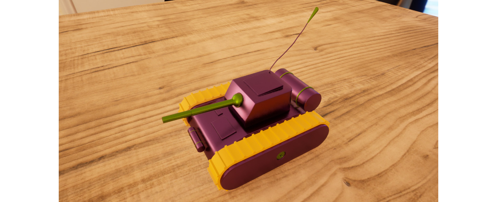
It’s time we looked at how to properly work with textures within a material, something that we’ll do now thanks to the small toy tank prop we’ve used in the last two recipes. The word properly is the key element in the previous sentence, for even though we’ve worked with images in the past, we haven’t really manipulated them inside the editor or seen how we can adjust them without leaving the editor. It’s time we did that, so let’s take care of it in this recipe!

Getting ready

You probably know the drill by now—just like in previous recipes, there’s not a lot that you’ll actually need in order to follow along. Most of the assets that we are going to be using can be acquired through the Starter Content asset pack, except for a few that we provide alongside this book’s Unreal Engine 5 project.

As you are about to see, we´ll continue using our famous toy tank model and material, so you can use either those or your own assets; we are dealing with fairly simple assets here, and the important bit is the actual logic that we are going to create within the materials.

If you want to along with me, feel free to open the level named 02_03_Start just so that we are looking at the same scene.

How to do it…

So far, all we’ve used in our toy tank material are simple colors—and even though they look good, we are going to make the jump to realistic textures this time. Let’s start:

1. Duplicate the material we created in the first recipe of this chapter, M_ToyTank. This is going to be useful, as we don’t want to reinvent the wheel so much as expand a system that already works. Having everything separated with masks and neatly organized will speed things up greatly this time. Name the new asset whatever you like—I’ve gone with M_ToyTank_Textured.
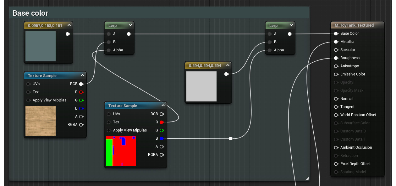
2. Open the material graph by double-clicking on the newly created asset and focus on the Base Color section of the material. Look for the Constant3Vector node that is driving the appearance of the main body of the tank (the one using a brownish shade) and delete it.
3. Create a new Texture Sample node and assign the T_Wood_Pine_D texture to it (this asset comes with the Starter Content asset pack, so we should already have access to it).
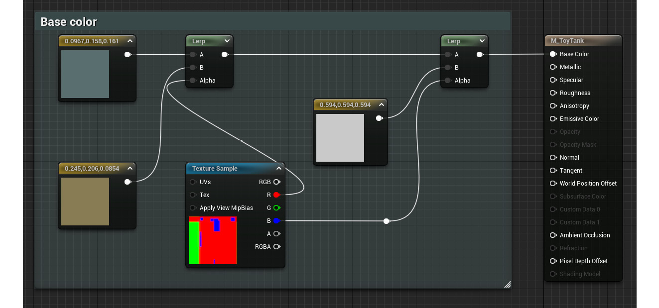
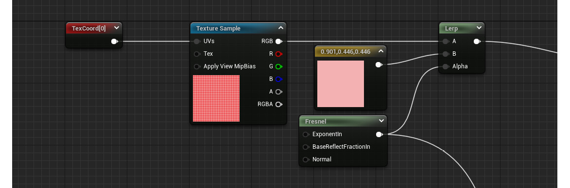
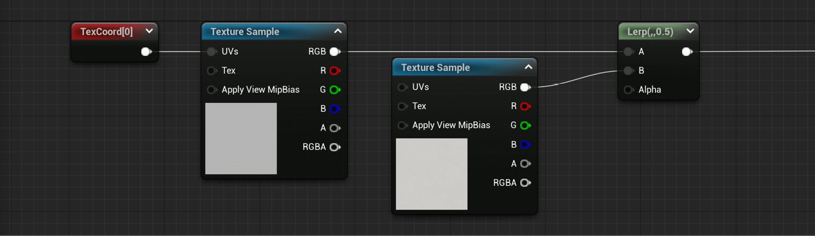
4. Connect the RGB output pin of the new Texture Sample node to the B input pin of the Lerp node, to which the recently deleted Constant3Vector node used to be connected:

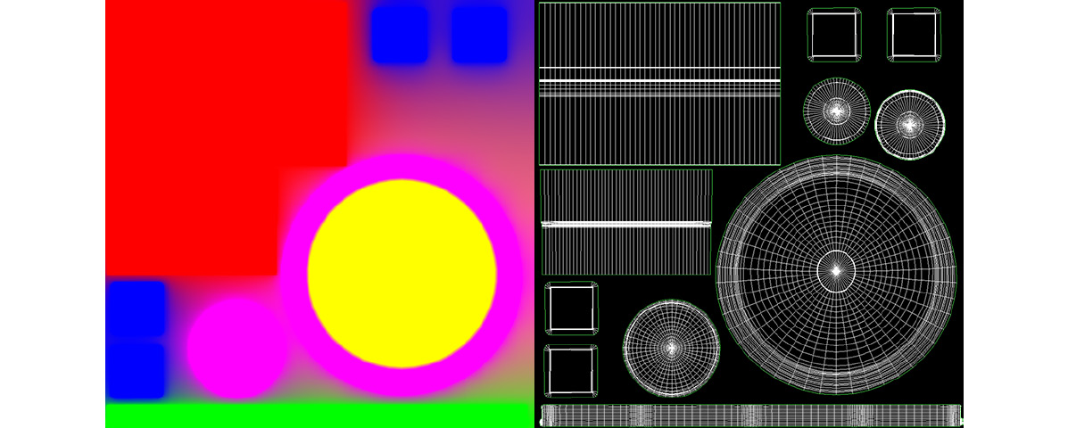
Figure 2.14 – The now-adjusted material graph

This will drive the appearance of the main body of the tank.

Tip

There’s a shortcut for the Texture Sample node: the letter T on your keyboard. Hold it and left-click anywhere within the material graph to create one.

There are a couple of extra things that we’ll be doing with this texture next—first, we can adjust the tiling so that the wood veins are a bit closer to each other once we apply the material to the model. Second, we might want to rotate it just to modify the current direction of the screenshot. Even though this is an aesthetic choice, it’s useful to get familiar with these nodes, as they are often quite useful when we need to use them.

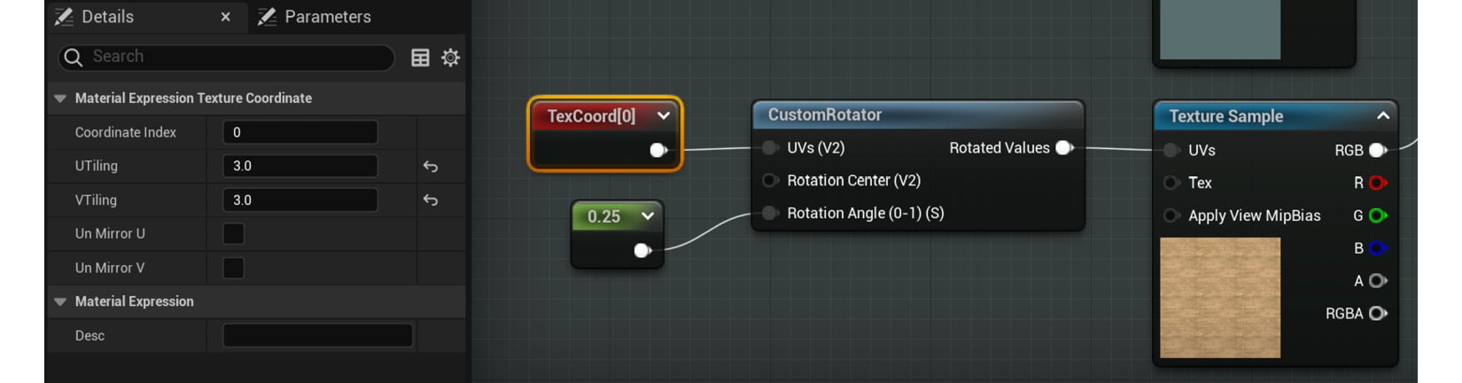
5. While holding down the U key on your keyboard, left-click in an empty space of the material graph to add a Texture Coordinate node. Assign a value of 3 to both its U Tiling and V Tiling settings, or adjust it until you are happy with the result.
6. Next, create a Custom Rotator node and place it immediately after the previous Texture Coordinate node.
7. With the previous node in place, plug the output of the Texture Coordinate node into the UVs (V2) input pin of the Custom Rotator node.
8. Connect the Rotated Values output node of the Custom Rotator node to the UVs input pin of the Texture Sample node used to display the wood texture.
9. Create a Constant node and plug it into the Rotation Angle (0-1) (S) node of the Custom Rotator node. Give it a value of 0.25 to rotate the texture 90 degrees (you can find more information regarding why a value of 0.25 equals 90 degrees in the How it works… section).

Here is what the previous sequence of nodes should look like:

Figure 2.15 – A look at the previous set of nodes

Let’s now continue to add a little extra variation to the other parts of the material. I’d like to focus on the other two masked elements next—the tires and the metallic sections—and make them a little bit more interesting visually speaking.

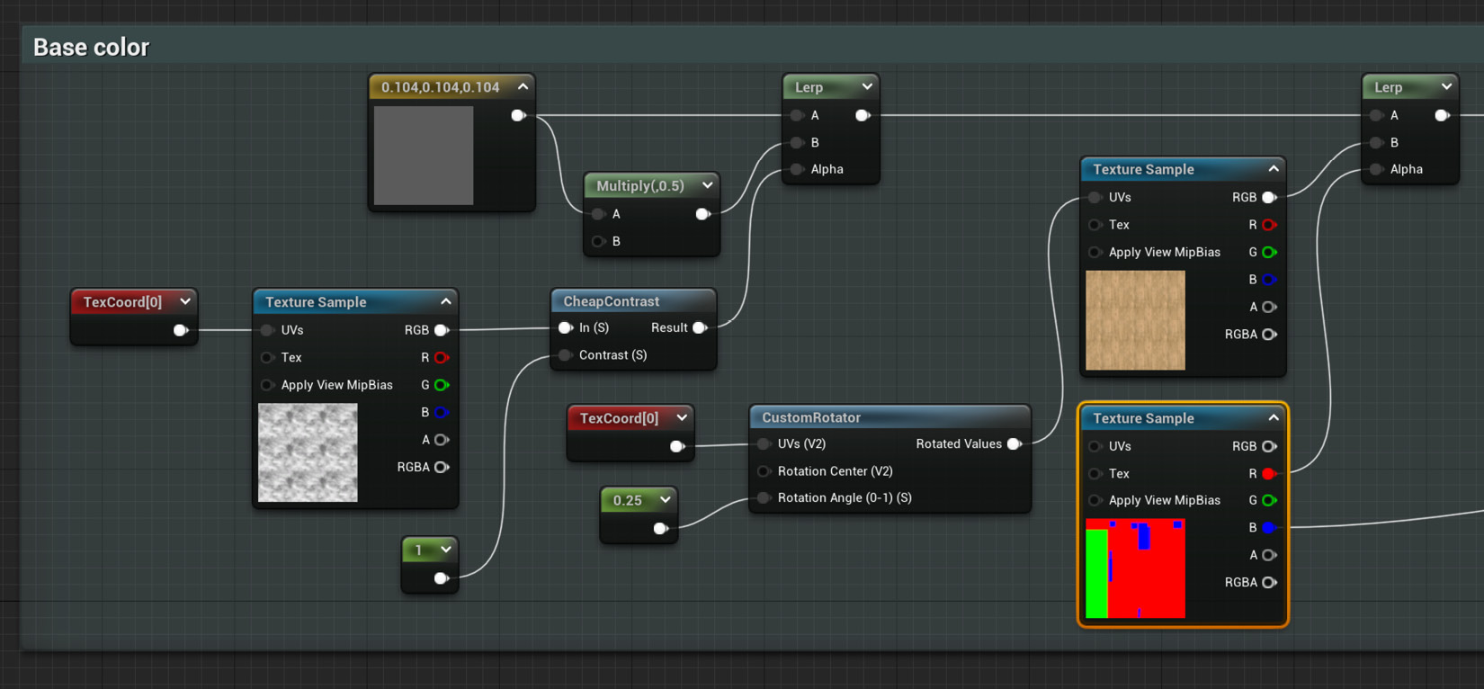
10. We can start by changing the color of the Constant3Vector node that we are using to drive the color of the toy tank’s tires to something that better represents that material (rubber). We’ve been using a blueish color so far, so something closer to black would probably be better.
11. After that, create a Multiply node and place it right after the previous Constant3Vector node. This is a very common type of node that does what its name implies: it outputs the result obtained after multiplying the inputs that reach this pin. One way to create it is by simply holding down the M key of the keyboard and left-clicking anywhere in the material graph.
12. With the previous Multiply node created, connect its A input pin to the output of the same Constant3Vector node driving the color of the rubber tires.
13. As for the B input pin, assign a value of 0.5 to it, something that you can do through the Details panel of the Multiply node without needing to create a new Constant node.
14. Interpolate between the default value of the Constant3Vector node for the rubber tires and the result of the previous multiplication by creating a Lerp node. You can do this by connecting the output of said Constant3Vector node to the A input pin of a new Lerp node and the result of the Multiply node to the B input pin. Don’t worry about the Alpha parameter for now—we’ll take care of that next.
15. Create a Texture Sample node and assign the T_Smoked_Tiled_D asset as its default value.
16. Next, create and connect a Texture Coordinate node to the previous Texture Sample node and assign a higher value than the default 1 to both its U Tiling and V Tiling parameters; I’ve gone with 3, just so that we can see the effect this will have more clearly in the future.
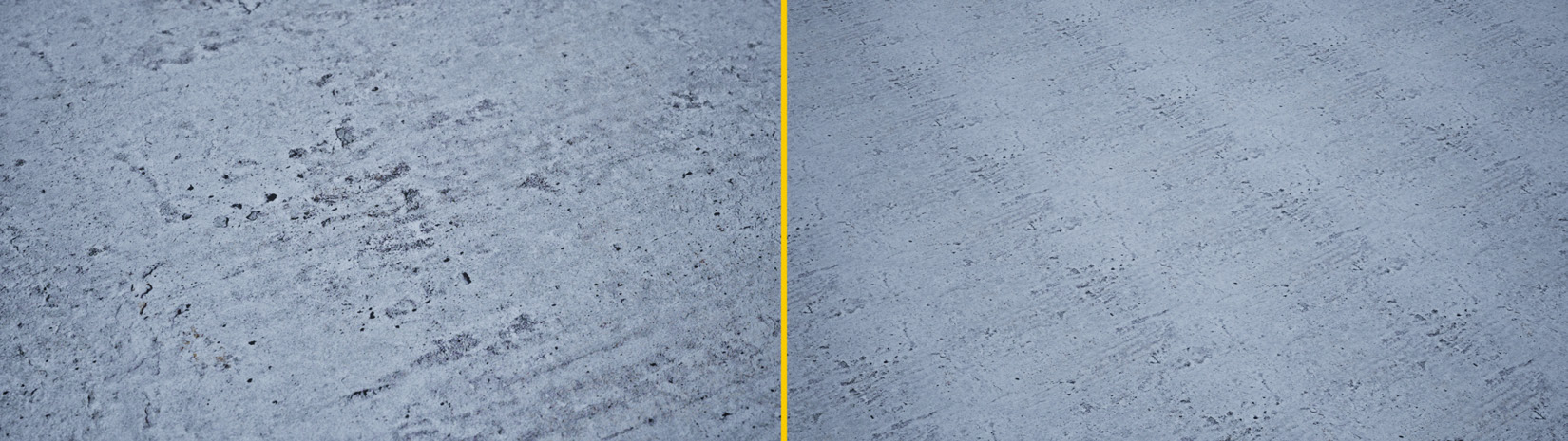
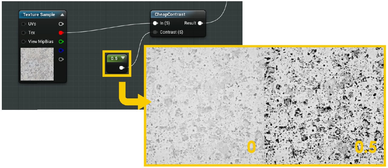
17. Proceed to drag a wire out of the output pin of the Texture Sample node for the new black-and-white smoke texture and create a Cheap Contrast node.
18. We’ll need to feed the previous Cheap Contrast node with some values, which we can do by creating a Constant node and connecting it to the Contrast (S) input pin of the previous node. This will increase the difference between the dark and white areas of the texture it is affecting, making the final effect more obvious. You can leave the default value of 1 untouched, as that will already give us the desired effect.
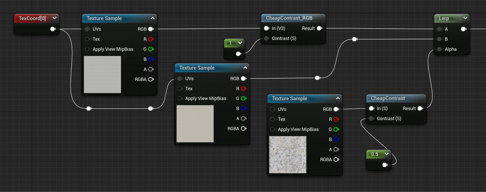
19. Connect the result of the Cheap Contrast node to the Alpha input pin of the Lerp node we created in step 14 and connect the output of that to the original Lerp node which is being driven by the T_TankMasks texture mask.

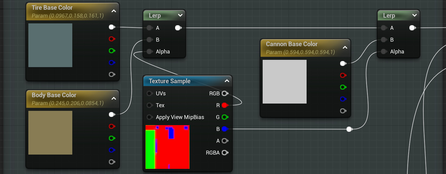
Here is a screenshot that summarizes the previous set of steps:

Figure 2.16 – The modified color for the toy tank tires

We’ve managed to introduce a little bit of color variation thanks to the use of the previous smoke texture as a mask. This is something that we’ll come back to in future recipes, as it’s a very useful technique when trying to create non-repetitive materials.

Tip

Clicking on the teapot icon in the Material Editor viewport will let you use whichever mesh you have selected on the Content Browser as the visible asset. This is useful for previewing changes without having to move back and forth between different viewports.

Finally, let’s introduce some extra changes to the metallic parts of the model.

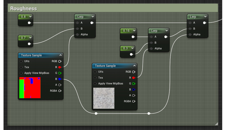
20. To do that, head over to the Roughness section of the material graph.
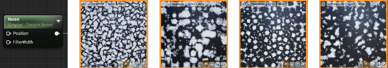
21. Create a Texture Sample parameter and assign the T_MacroVariation texture to it. This will serve as the Alpha pin for the new Lerp node we are about to create.
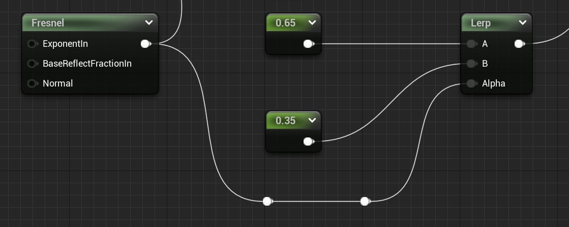
22. Add two simple Constant nodes and give them two different values. Keep in mind that these will affect the roughness of the metallic parts when choosing the values, so values lower than 0.3 will work well when making those parts reflective.
23. Place a new Lerp node and plug the previous two new Constant nodes into the A and B input pins.
24. Connect the red channel of the Texture Sample node we created in step 21 to the Alpha input pin of the previous Lerp node.

Important note

The reason why we are connecting the red channel of the previous Texture Sample node to the Alpha input pin of the Lerp node is simply that it offers a grayscale value which we can use in our favor to drive the mixture of the different roughness values.

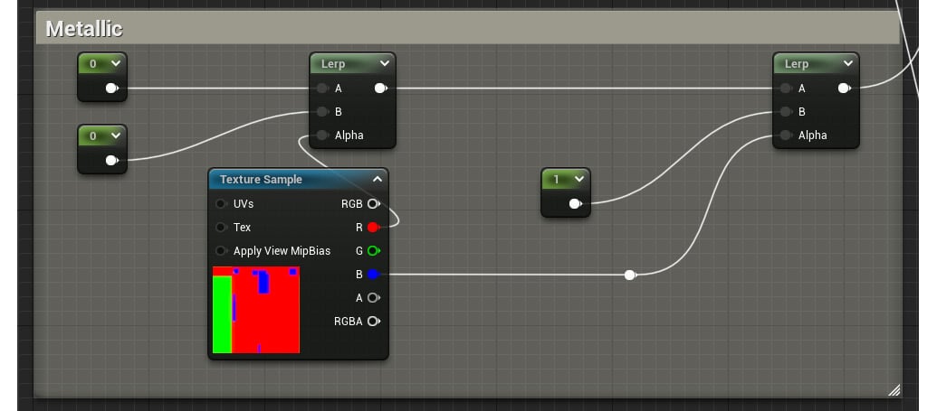
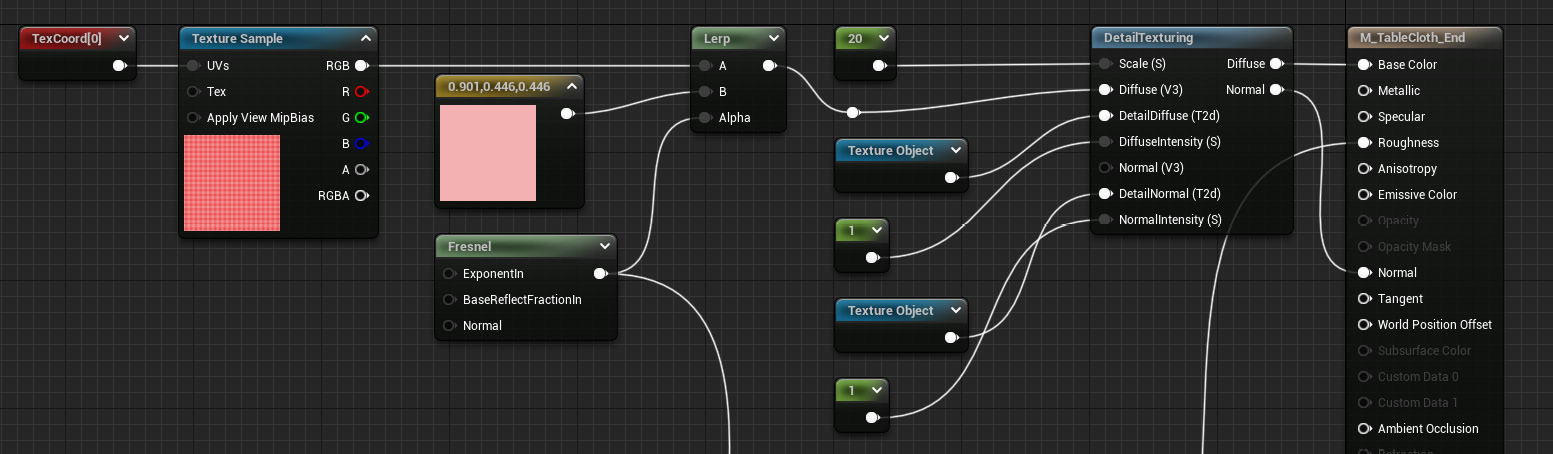
25. Finally, replace the initial Constant that was driving the roughness value of the metallic parts with the node network we created in the three previous steps. The graph should now look something like this:

Figure 2.17 – The updated roughness section of our material

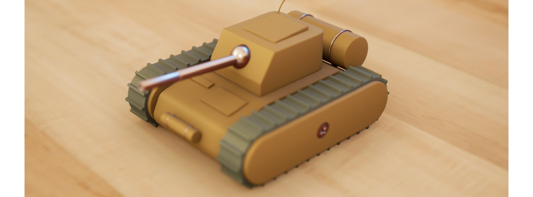
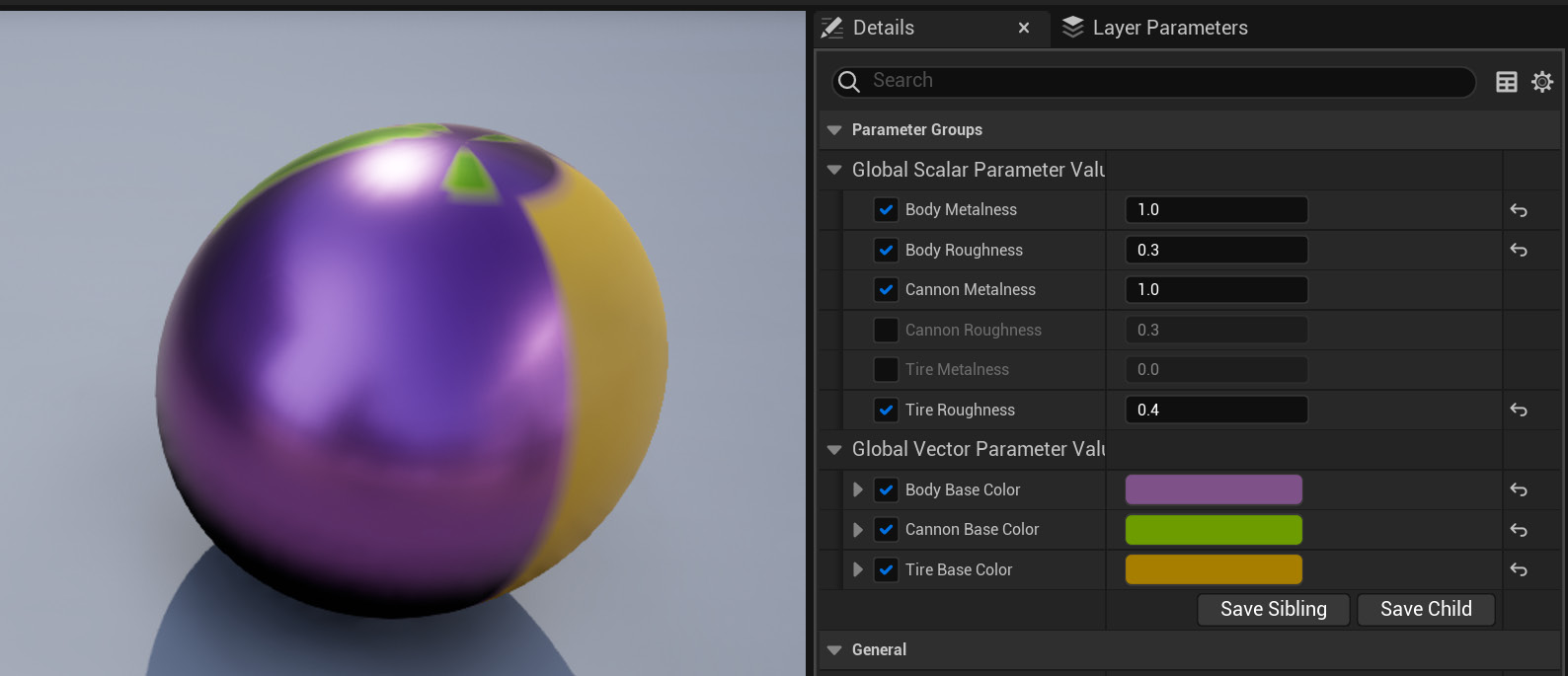
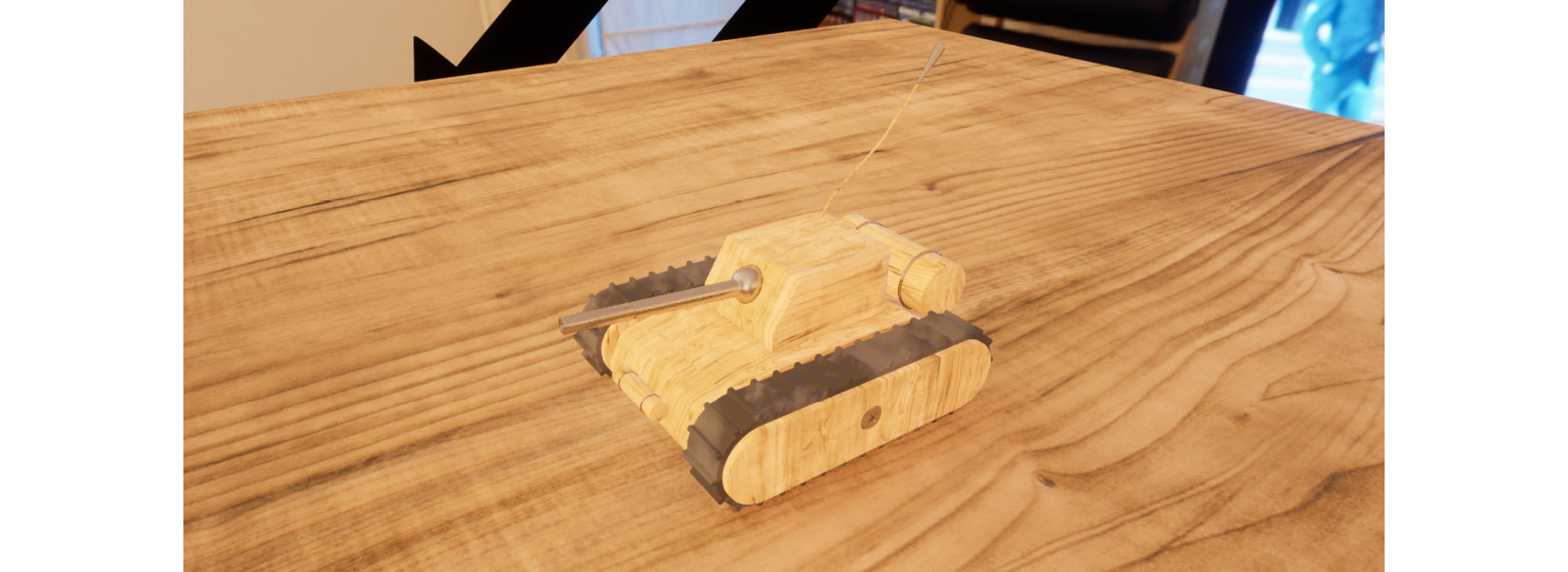
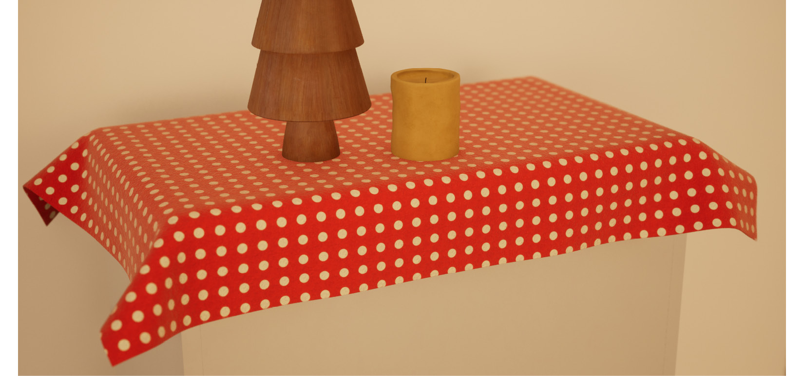
And after doing that, let’s now... oh, wait; I think we can call it a day! After all of those changes have been made, we will be left with a nice new material that is a more realistic version of the shader we had previously created. Furthermore, everything we’ve done constitutes the basics of setting up a real material in Unreal Engine 5. Combining textures with math operations, blending nodes according to different masks, and taking advantage of different assets to create specific effects are everyday tasks that many artists working with the engine have to face. And now, you know how to do that as well! Let’s check out the results before moving on:

Figure 2.18 – The final look of the textured toy tank material

How it works…

We’ve had the opportunity to look at several new nodes in this recipe, so let’s take a moment to review what they do before moving forward.

One of the first ones we used was the Texture Coordinate one, which affects the scaling of the textures that we apply to our models. The Details panel gives us access to a couple of parameters within it, U Tiling and V Tiling. Modifying those settings will affect the size of the textures that are affected by this node, with higher values making the images appear smaller. In reality, the size of the textures doesn’t really change, as their resolution stays the same: what changes is the amount of UV space that they occupy. A value of 1 for both the U Tiling and the V Tiling parameters means that any textures connected to the Texture Coordinate node occupy the entirety of the UV space, while a value of 2 means that the same texture is repeated twice over the same extent. Decoupling the U Tiling parameter from the V Tiling parameter lets us affect the repetition pattern independently on those two axes, giving us a bit more freedom when adjusting the look of our materials.

Important note

There’s a third parameter that we can tweak within the Texture Coordinate node— Coordinate Index. The value specified in this field affects the UV channel we are affecting, should we use more than one.

On that note, it’s probably important to highlight the importance of well-laid-out UVs. Seeing as how many of the nodes that we’ve used directly affect the UV space, it only makes sense that the models with which we work contain correctly unwrapped UV maps. Errors here will most likely impact the look of any textures that you try to apply, so make sure to check for mistakes in this area.

Another node that we used to modify the textures used in this recipe was the Custom Rotator node. This one adjusts the rotation of the images you are using, so it’s not very difficult to conceptualize. The trickiest setting to wrap our heads around is probably the Constant that drives the Rotation Angle (0-1) (S) parameter, which dictates the degrees by which we rotate a given texture. We need to feed a value within the 0 to 1 range, 0 being no rotation and 1 mapping to 360 degrees. A value of 0.25, the one we used in this recipe, corresponds exactly to 90 degrees following a simple rule of three.

Something that we can also affect using the Custom Rotator node are the UVs of the model, just as we did with the Texture Coordinate node before (in fact, we plugged the latter into the UVs (V2) input pin of the former). This allows us to increase or decrease the repetition of the texture before we rotate it. Finally, the Rotation Centre (V2) parameter allows us to determine the center of the rotation. This works according to the UV space, so a value of (0,0) will see the texture rotating around its bottom-left corner, a value of (0.5,0.5) will rotate the image around its center, and a value of (1,1) will do the same around the upper-right corner.

The third node we will discuss is the Multiply one. It is rather simple in terms of what it does: it multiplies two different values. The two elements need to be of a similar nature —we can only multiply two Constant3Vector nodes, two Constant2Vector nodes, two Texture Sample nodes, and so on. The exception to this rule is the simple Constant nodes, which can always be combined with any other input. The Multiply node is often used when adjusting the brightness of a given value, which is what we’ve done in this recipe.

Finally, the last new node we saw was Cheap Contrast. This is useful for adjusting the contrast of what we hook into it, with the default value of 0 not adjusting the input at all. We can use a constant value to adjust the intensity of the operation, with higher values increasing the difference between the black and the white levels. This particular node works with grayscale values—should you wish to perform the same operation in a colored image, note that there’s another CheapContrast_RGB node that does just that.

Tip

A useful technique that lets you evaluate the impact of the nodes you place within the material graph is the Start Previewing Node option. Right-click on the node that you want to preview and choose that option to start displaying the result of the node network you’ve chosen up to that point. The results will become visible in the viewport.

See also

I want to leave you with a couple of links that provide more information regarding Multiply, Cheap Contrast, and some other related nodes:

• https://docs.unrealengine.com/4.27/en-US/RenderingAndGraphics/Materials/Functions/Reference/ImageAdjustment/
• https://docs.unrealengine.com/4.27/en-US/RenderingAndGraphics/Materials/ExpressionReference/Math/

We started to use textures extensively in the previous recipe, and we also had the opportunity to talk about certain useful nodes, such as Cheap Contrast and Custom Rotator. Just as with those two, Unreal includes several more that have been created to suit the needs of 3D artists, with the goal of sometimes improving the look of our models or creating specific effects in a smart way. Whatever the case, learning about them is sure to improve the look of our scenes.

We’ll be looking at some of those useful nodes in this recipe, paying special attention to the Fresnel one, which we’ll use to achieve a velvety effect across the 3D model of a tablecloth—something that would be more difficult to achieve without it. Let’s jump straight into it!

Getting ready

The scene we’ll be using in this recipe is a bit different from the ones we’ve used before. Rather than a toy tank, I thought it would be good to change the setting and have something on which we can demonstrate the new techniques we are about to see, so we’ll use a simple cloth to highlight these effects. Please open 02_04_Start if you want to follow along with me.

If you want to use your own assets, know that we’ll be creating a velvet-like material in this recipe, so it would be great to have an object onto which you can apply that.

How to do it…

We are about to take a simple material and enhance it using some of the material nodes available in Unreal, which will help us—with very little effort on our side—to improve its final appearance.

1. First of all, let’s start by loading the 02_04_Start level and opening the material that is being applied to the tablecloth, named M_TableCloth_Start, as we are going to be working on that one. As you can see, it only has a single Constant3Vector node modifying the Base Color property of the material, and that’s where we are going to start working.
2. Next, create a Texture Sample node and assign the T_TableCloth_D texture to it.
3. Add a Texture Coordinate node and connect it to the input pin of the previous Texture Sample node. Set a value of 20 for both its U Tiling and V Tiling properties.
4. Proceed to include a Constant3Vector node and assign a soft red color to it, something similar but lighter to the color of the texture chosen for the existing Texture Sample node. I’ve gone with the following RGB values: R = 0.90, G = 0.44, and B = 0.44.
5. Moving on, create a Lerp node and place it after both the original Texture Sample node and the new Constant3Vector node.
6. Connect the previous Texture Sample node to the A input pin of the new Lerp node, and wire the output of the Constant3Vector node to the B input pin.
7. Right-click anywhere within the material graph and type Fresnel to create that node. Then, connect the output of the Fresnel node to the Alpha input pin of the previous Lerp node.

This new node tries to mimic the way light reflects out of the objects it interacts with, which varies according to the viewing angle at which we see those surfaces—with areas parallel to our viewing angle having clearer reflections.

Having said that, let’s look at the next screenshot, which shows the material graph at this point:

Figure 2.19 – A look at the current state of the material graph

8. Select the Fresnel node and head over to the Details panel. Set the Exponent parameter to something lower than the default, which will make the effect of the Fresnel function more apparent. I’ve gone with 2.5, which seems to work fine for our purposes.

Next up, we are going to start using another new different node: the Detail Texturing one. This node allows us to use two different textures to enhance the look of a material. Its usefulness resides in the ability to create highly detailed models without the need for large texture assets. Of course, there might be other cases where this is also useful beyond the example I’ve just mentioned. Let’s see how to set it up.

9. Right-click within the material graph and type Detail Texturing. You’ll see this new node appear.
10. In order to work with this node, we are going to need some extra ones as well, so create three Constant nodes and two Texture Sample nodes.
11. Proceed to connect the Constant nodes to the Scale, Diffuse Intensity, and Normal Intensity input pins. We’ll worry about the values later.
12. Set T_ground_Moss_D and T_Ground_Moss_N as the assets in the Texture Sample nodes we created (they are both part of the Starter Content asset pack).

Important note

Using the Detail Texturing node presents a little quirk, in that the previous two Texture Sample nodes that we created will need to be converted into what is known as a Texture Object node More about this node type in the How it works… section.

13. Right-click on the two Texture Sample nodes and select Convert to Texture Object.
14. Give the first Constant node—the one connected to the Scale pin—a value of 20, and assign a value of 1 to the other Constant nodes.
15. Connect the Diffuse output pin of Detail Texturing to the Base Color input pin in the main material node, and hook the Normal output of the Detail Texturing node to the Normal input pin of our material.

This is what the material graph should look like now:

Figure 2.20 – The material graph with the new nodes we’ve just added

Before we finish, let’s continue working a bit longer and reuse the Fresnel node once again to drive the Roughness parameter of the material. The idea is to use it to specify the roughness values, making the parts that are facing the camera have less clear reflections than the parts that are facing away from it.

16. Create two Constant nodes and give them different values—I’ve gone with 0.65 and 0.35 this time. The first of those values will make the areas where it gets applied appear rougher, which will happen when we look directly at the surface by virtue of using the Fresnel node. Following the same principle, the second one will make the areas that face away from us have clearer reflections.
17. Add a Lerp node and connect the previous Constant nodes to its A and B pins. The rougher value (0.65) should go into the A input pin, while the second one should be fed into the B pin.
18. Drag another pin from our original Fresnel node and hook it to the Alpha input pin of the new Lerp node.
19. Connect the output of the Lerp node to the Roughness parameter in the main material node.

The final graph should look something along these lines:

Figure 2.21 – The final addition to the material graph

Finally, all we need to do is to click on the Apply and Save buttons and assign the material to our model in the main viewport. Take a look at what we’ve created and try to play around with the material, disconnecting the Fresnel node and seeing what its inclusion achieves. It is a subtle effect, but it allows us to achieve slightly more convincing results that can trick the eye into thinking that what it is seeing is real. You can see this in the following screenshot when looking at the cloth: the top of the model appears more washed out because it is reflecting more light, while the part that faces the camera appears redder:

Figure 2.22 – The final look of the cloth material

How it works…

Let’s take a minute to understand how the Fresnel node works, as it can be tricky to grasp. This effect assigns a different value to each pixel of an object depending on the direction that the normal at that point is facing. Surface normals perpendicular to the camera (those pointing away from it) receive a value of 1, while the ones that look directly at it get a value of 0. This is the result of a dot product operation between the surface normal and the direction of the camera that results in a falloff effect we can adjust with the three input parameters present in that node:

• The first of them, ExponentIn, controls the falloff effect, with higher values pushing it toward the areas that are perpendicular to the camera.
• The second, BaseReflectFrctionIn, specifies “the fraction of specular reflection when the surface is viewed from straight on,” as stated by Unreal. This basically specifies how the areas that are facing the camera behave, so using a value of 1 here will nullify the effect of the node.
• The third, Normal, lets us provide a normal texture to adjust the apparent geometry of the model the material is affecting.

Detail Texturing is also a handy node to get familiar with, as seen in this example. But even though it’s quite easy to use, we could have achieved a similar effect by implementing a larger set of nodes that consider the distance to a given object and swap textures according to that. In fact, that is the logic that you’ll find if you double-click on the node itself, which isn’t technically a node but a Material Function. Doing that will open its material graph, letting you take a sneak peek at the logic driving this function. As we see in there, it contains a bunch of nodes that take care of creating the effect that we end up seeing playing its part in the material we created. Since these are normal nodes, you can copy and paste them into your own material. Doing that would remove the need to use the Detail Texturing node itself, but this also highlights why we use Material Functions in the first place: they are a nice way of reusing the same logic across different materials and keeping things organized at the same time.

Finally, I also wanted to touch base on the Texture Object node we encountered in this recipe. There can be a bit of confusion around this node, as it is apparently similar to the Texture Sample one—after all, we used both types to specify a texture, which we then used in our material. The difference is that Texture Object nodes are the format in which we send textures to a Material Function, which we can’t do using Texture Sample nodes. If you remember, we used Texture Object nodes alongside the Detail Texturing node, which was a Material Function itself—hence the need to use Texture Object nodes. We also sent the information of the Texture Sample node used for the color, but the Detail Texturing node sampled that as Vector3 information and not as a Texture node. You can think of Texture Object nodes as references to a given texture, while the Texture Sample node represents the values of that given texture (its RGB information as well as the Alpha input pin and each of the texture’s channels).

See also

You can find more documentation about the Fresnel and Detail Texturing nodes through Epic’s official documents:

• https://docs.unrealengine.com/4.27/en-US/RenderingAndGraphics/Materials/HowTo/Fresnel/
• https://docs.unrealengine.com/4.27/en-US/RenderingAndGraphics/Materials/HowTo/DetailTexturing/

Thus far, we’ve only worked with materials that we have applied to relatively small 3D models, where a single texture or color was enough to make them look good. However, that isn’t the only type of asset that we’ll encounter in a real-life project. Sometimes we will have to deal with bigger meshes, making the texturing process not as straightforward as we’ve seen so far. In those circumstances, we are forced to think creatively and find ways to make that asset look good, as we won’t be able to create high enough resolution textures that can cover the entirety of the object.

Thankfully, Unreal provides us with a very robust Material Editor and several ways of tackling this issue, as we are about to see next through the use of semi-procedural material creation techniques. This approach to the material-creation process relies on standard effects that aim to achieve a procedural look—that is, one that seems to follow mathematical functions in its operation rather than relying on existing textures. This is done with the intention of alleviating the problems inherent to using those assets, such as the appearance of obvious repetition patterns. This is what we’ll be doing in this recipe.

Getting ready

We are about to use several different assets to semi-procedurally texture a 3D model, but all the resources that you will need to use come bundled within the Starter Content asset pack in Unreal Engine 5. Be sure to include it if you want to follow along using the same textures and models I’ll be using, but don’t worry if you want to use your own, as everything we are about to do can be done using very simple models.

As always, feel free to open the scene named 02_05_ Start if you are working on the Unreal project provided alongside this book.

How to do it…

Let’s start this recipe by loading the 02_05_ Start level. Looking at the object at the center of the screen, you’ll see a large plane that acts as a ground floor, which has been placed there just so that we can see the problems that arise when using textures to shade a large-scale surface—as evidenced by the next screenshot:

Figure 2.23 – A close-up look at the concrete floor next to a faraway shot showing the repetition of the same pattern over the entirety of the surface

As you can see, the first image in the screenshot could actually be quite a nice one, as we have a concrete floor that looks convincing. However, the illusion starts to fall apart once the camera gets farther from the ground plane. Even though it might be difficult to notice at first, the repetition of the texture across the surface starts to show up. This is what we are going to try to fix in this recipe: creating materials that look good both up close and far from the camera, all thanks to semi-procedural material creation techniques. Let’s dive right in:

1. Open the material being applied to the plane, M_SemiProceduralConcrete_Start. You should see a lonely Texture Sample node (T_Concrete_Poured_D) being driven by a Texture Coordinate node, which is currently adjusting the tiling. This will serve as our starting point.
2. Add another Texture Sample node and set the T_Rock_Marble_Polished_D texture from the Starter Content asset pack as its value. We are going to blend between these first two images thanks to the use of a third one, which will serve as a mask.

Using multiple similar assets can be key to creating semi-procedural content. Blending between two or more textures into a random pattern helps alleviate the visible tiling across big surfaces.

3. Connect the output of the existing Texture Coordinate node to the UVs input pin of the previous Texture Sample node we created.

The next step will be to create a Lerp node, which we can use to blend between the first two images. We want to use a texture that has a certain randomness to it, and the Starter Content asset pack includes one named T_MacroVariation that could potentially work. However, we’ll need to adjust it a little bit, as it currently has a lot of gray values that wouldn’t work too well for masking purposes. Using it in its current state would have us blend between two textures simultaneously when we really want to use one or the other based on the previous texture.Let’s adjust the texture to achieve that effect.

4. Create a new Texture Sample node and assign the T_MacroVariation asset to it.
5. Include a Cheap Contrast node after the previous Texture Sample node and hook its input pin to the output of the said node.
6. Add a Constant node and connect it to the Contrast slot in the Cheap Contrast node. Give it a value of 0.5 so that we achieve the desired effect we mentioned before.

Here is a screenshot of what we should have achieved through this process:

Figure 2.24 – The previous set of nodes and their result

7. Create a Lerp node, which we’ll use in the next step to combine the first two Texture Sample nodes according to the mask we created in the previous step.
8. Connect the output nodes of the first two texture assets (T_Rock_Marble_Polished_D and T_Concrete_Poured_D) to the A and B input pins of the Lerp node and connect the Alpha input pin to the output pin of the Cheap Contrast node. The graph should look something like this:

Figure 2.25 – The look of the material graph so far

We’ve managed to add variety and randomness to our material thanks to the nodes we created in the previous steps. Despite that, there’s still room for improvement, as we can take the previous approach one step further. We will now include a third texture, which will help further randomize the shader, as well as give us the opportunity to further modify an image within Unreal.

9. Create a new couple of nodes—a Texture Coordinate node and a Texture Sample one.
10. Assign the T_Rock_Sandstone_D asset as the default value of the Texture Sample node, and give the Texture Coordinate node a value of 15 in both the U Tiling and V Tiling fields.
11. Continue by adding a Desaturation node and a Constant node right after the previous Texture Sample node. Give the Constant node a value of 0.8 and connect it to the Fraction input pin of the Desaturation node, whose job is to desaturate or remove the color from any texture we provide it, creating a black-and-white version of the same asset instead.
12. Connect the output of the Texture Sample node to the Desaturation node.

This is what we should be looking at:

Figure 2.26 – The effect of the Desaturation node

Following these steps has allowed us to create a texture that can work as concrete, but that really wasn’t intended as such. Nice! Let’s now create the final blend mask.

13. Start by adding a new Texture Sample node and assign the T_MacroVariation texture as its default value.
14. Continue by including a Texture Coordinate node and give it a value of 2 in both its U Tiling and V Tiling parameters.
15. Next, add a Custom Rotator node and connect its UVs input pin to the output of the previous Texture Coordinate one.
16. Create a Constant node and feed it to the Rotation Angle input pin of the Custom Rotator node. Give it a value of 0.167, which will rotate the texture by 60 degrees.

Important note

You might be wondering why a value of 0.167 translates to a rotation of 60 degrees. This is for the same reason we saw a couple of recipes ago—the Custom Rotator node maps the 0-to-360-degree range to another one that goes from 0 to 1. This makes 0.167 roughly 60 degrees: 60.12 degrees if we want to be precise!

17. Hook the Custom Rotator node into the UVs input pin of the Texture Sample node.
18. Create a new Lerp node and feed the previous Texture Sample node into the Alpha input pin.
19. Connect the A pin to the output of the original Lerp node and connect the B pin to the output of the Desaturation node.
20. Wire the output of the previous Lerp node to the Base Color input pin in the main material node. We’ve now finished creating random variations for this material!

One final look at the plane in the scene with the new material applied to it should give us the following result:

Figure 2.27 – The final look of the material

The final shader looks good both up close and far away from the camera. This is happening thanks to the techniques we’ve used, which help reduce the repetition across our 3D models quite dramatically. Be sure to remember this technique, as I’m sure it will be quite handy in the future!

How it works…

The technique we used in this recipe is quite straightforward—just introduce as much randomness as you can until the eye gets tricked into thinking that there’s no single texture repeating endlessly. Even though this principle can be simple to grasp, it is by no means simple—humans are very good at recognizing patterns, and as the surfaces we work on increase in size, so does the challenge.

Choosing the right textures for the job is part of the solution—be sure to blend gently between different layers, and don’t overuse the same masks all the time. Doing so could result in our brains figuring out what’s going on. This is a method that has to be used gently.

Focusing now on the new nodes that we used in this recipe, we probably need to highlight the Desaturation one. It is very similar to what you might have encountered in other image-editing programs: it takes an image and gradually takes the “color” away from it. I know these are all very technical terms—not!—but that is the basic idea. The Unreal node does the same thing: we start from an RGB image and we use the Fraction input to adjust the desaturation of the texture. The higher the value, the more desaturated the result. Simple enough!

Something else that I wanted to mention before we move on is the real procedural noise patterns available in Unreal. In this recipe, we created what can be considered semi-procedural materials through the use of several black-and-white gradient-noise textures. Those are limited in that they too repeat themselves, just like the images we hooked to the Base Color property—it was only through smart use of them that we achieved good enough results. Thankfully, we have access to the Noise node in Unreal, which gets rid of that limitation altogether. You can see some examples here:

Figure 2.28 – The Noise node and several of its available patterns

This node is exactly what we are looking for to create fully procedural materials. As you can see, it creates random patterns, which we can control through the settings in the Details panel, and the resulting maps are similar to the masks we used in this recipe.

The reason why we didn’t take advantage of this asset is that it is quite taxing with regard to performance, so it is often used to create nice-looking materials that are then baked. We’ll be looking at material-baking techniques in a later chapter, so be sure to check it out!

See also

You can find an extensive article on the Noise node at the following link:

https://www.unrealengine.com/es-ES/tech-blog/getting-the-most-out-of-noise-in-ue4

It’s also a great resource if you want to learn more about procedural content creation, so be sure to give it a go!

We are now going to learn how to blend between a couple of different textures according to how far we are from the model to which they are being applied. Even though it’s great to have a complex material that works both when the camera is close to the 3D model and when we are far from it, such complexity operating on a model that only occupies a small percentage of our screens can be a bit too much. This is especially true if we can achieve the same effect with a much lower-resolution texture.

With that goal in mind, we are going to learn how to tackle those situations in the next few pages. Let’s jump right in!

Getting ready

If we look back at the previous recipe, you might remember that the semi-procedural concrete material we created made use of several nodes and textures. This serves us well to prove the point that we want to make in the next few pages: achieving a similar look using lower-resolution images and less complex graphs. We will thus start our journey with a very similar scene to what we have already used, named 02_06_Start.

Right before we start, though, know that I’ve created a new texture for you, named T_DistantConcrete_D, which we’ll be using in this recipe. The curious thing about this asset is that it’s a baked texture from the original, more complex material we used in the Creating semi-procedural materials recipe. We’ll learn how to create these simplified assets later in the book when we deal with optimization techniques.

How to do it…

Let’s jump right into the thick of it and learn how to blend between textures based on the distance between the camera and the objects to which these images are being applied:

1. Let’s start by creating a new material and giving it a name. I’ve chosen M_DistanceBasedConcrete, as it roughly matches what we want to do with it. Apply it to the plane in the center of the level. This is the humble start of our journey!
2. Continue by adding two Texture Sample nodes, and choose the T_Concrete_Poured_D and the T_DistantConcrete_D images as their default values.
3. Next, include a Texture Coordinate node and plug it into the first of the two Texture Sample nodes. Assign a value of 20 to its two parameters, U Tiling and V Tiling.
4. Place a Lerp node in the graph and connect its A and B input pins to the previous Texture Sample nodes. This is how the graph should look up to this point:

Figure 2.29 – The material graph so far

Everything we’ve done so far was mixing two textures, one of which we already used in the previous recipe. The idea is to create something very similar to what we previously had, but more efficient. The part that we are now going to tackle is distance-based calculations, as we’ll see next.

5. Start by creating a World Position node, something that can be done by right-clicking anywhere within the material graph and typing its name. This new node allows us to access the world coordinates of the model to which the material is being applied, enabling us to create interesting effects such as tiling textures without considering the UVs of a model.

Important note

The World Position node can have several prefixes (Absolute, Camera Relative…) based on the mode we specify for it in the Details panel. We want to be working with its default value—the Absolute one.

6. Create a Camera Position node. Even though that’s the name that appears in the visual representation of that function, the name that will show up when you look for it will be Camera Position WS (WS meaning World Space).
7. Include a Distance node after the previous two, which will give us the value of the separation between the camera and the object that has this material applied to it. You can find this node under the Utility section. Connect the Absolute World Position node to its A input pin, and the Camera Position one to the B input.
8. Next, add a Divide node and a Constant node. You can find the first node by just typing that name, or alternatively by holding down the D key on your keyboard and clicking in an empty space of the material graph. Incidentally, Divide is a new node that allows us to perform that mathematical operation on the two inputs that we need to provide it with.
9. Give the Constant node a value of something such as 256. This will drive the distance from the camera at which the swapping of the textures will happen. Higher numbers mean that it will be further from the camera, but this is something that has to be interactively tested to narrow down the precise sweet spot at which you want the transition to happen.
10. Add a Power node after the previous Divide node and connect the result of the latter to the Base input pin of the former. Just as with the Divide node, this function performs the homonymous mathematical operation according to the values that we provide it with.
11. Create another Constant node, which we’ll use to feed the Exp pin of the Power node. The higher the number, the softer the transition between the two textures. Sensible numbers can be anything between 1 to 10 – I’ve chosen 4 this time.
12. Include a Clamp node into the mix at the end, right after the final Power node, and connect both. Leave the values at their default, with 0 as the minimum and 1 as the maximum.
13. Connect the output pin of the previous Clamp node to the Lerp node that we used to blend between the two textures acting as the Base Color node, the one we created in step 4.

The graph we’ve created should now look something like this:

Figure 2.30 – The logic behind the distance-blending technique used in this material

We should now have a material that can effectively blend between two different assets according to the distance at which the model is from the camera. Of course, this approach could be expanded upon and made so that we are not just blending between two textures, but between as many as we want. However, one of the benefits of using this technique is to reduce the rendering cost of materials that were previously too expensive to render—so, leaving things relatively simple will help work in our favor this time.

Let me leave you with a screenshot that highlights the results both when the camera is up close and when it is far away from our level’s main ground plane:

Figure 2.31 – Comparison shots between the close-up and distant versions of the material

As you can see, the differences aren’t that big, but we are using fewer textures in the new material compared to the previous one. That’s a win right there!

Tip

Try to play around with the textures used for the base color and the distance values used in the Constant node created in steps 8 and 9 to see how the effect changes. Using bright colors will help highlight what we are doing, so give that a go in case you have trouble visualizing the effect!

How it works…

We can say that we’ve worked with a few new nodes in this recipe—Absolute World Position, Distance, Camera Position, Divide, Power, Clamp… We did go over all of them a few pages ago, but it’s now time to delve a little bit deeper into how they operate.

The first one we saw, the Absolute World Position node, gives us the location of the vertices we are looking at in world space. Pairing it with the Camera Position and Distance nodes we used immediately after allowed us to know the distance between our eyes and the object onto which we applied the material—the former giving us the value for the camera location and the latter being used to compare the positional values we have.

We divided the result of the Distance node by a Constant using the Divide node, a mathematical function similar to the Multiply node that we’ve already seen. We did this in order to adjust the result we got out of the Distance node—to have a value that was easier to work with.

We then used the Power node to drive the mathematical operation, which allowed us to create a softer transition between the two textures that we were trying to blend. In essence, the Power node simply executes said operation with the data that we provide it. Finally, the Clamp node took the value we fed to it and made sure that it was contained within the 0 to 1 range that we specified for it—so, any higher values than the unit would have been reduced to one, while lower values than zero would have been increased to zero.

All the previous operations are mathematical in nature, and even though there are not that many nodes involved, it would be nice if there were a way for us to visualize the values of those operations. That would be helpful with regard to knowing the values that we should use—you can imagine that I didn’t just get the values that we used in this recipe out of thin air, but rather after careful consideration.

There are some extra nodes that can be helpful in that regard, all grouped within the Debug category. Elements such as DebugScalarValues, DebugFloat2Values, and others will help you visualize the values being computed in different parts of the graph. To use them, simply connect them to the part of the graph that you want to analyze and wire their output to the Base Color input pin node of the material. Here is an example of using the DebugScalarValues node at the end of the distance blend section of the material we’ve worked on in this recipe:

Figure 2.32 – The effects of using debug nodes to visualize parts of the graph

See also

You can find extra information about some of the nodes we’ve used, such as Absolute World Position, in Epic Games’ official documentation:

https://docs.unrealengine.com/en-US/Engine/Rendering/Materials/ExpressionReference/Coordinates

There are some extra nodes in there that might catch your eye, so make sure to check them out!