


Adding subplots
Occasionally, it is useful to place multiple related plots within the same figure side by side but not on the same axes. Subplots allow us to produce a grid of individual plots within a single figure. In this recipe, we will see how to create two plots side by side on a single figure using subplots.
Getting ready
You will need the data to be plotted on each subplot. As an example, we will plot the first five iterates of Newton’s method applied to the  function with an initial value of
  on the first subplot, and for the second, we will plot the error of the iterate. We first define a generator function to get the iterates:
def generate_newton_iters(x0, number):
  iterates = [x0]
  errors = [abs(x0 - 1.)]
  for _ in range(number):
       x0 = x0 - (x0*x0 - 1.)/(2*x0)
       iterates.append(x0)
       errors.append(abs(x0 - 1.))
    return iterates, errors
This routine generates two lists. The first list contains iterates of Newton’s method applied to the function, and the second contains the error in the approximation:
iterates, errors = generate_newton_iters(2.0, 5)
How to do it...
The following steps show how to create a figure that contains multiple subplots:
- We use the
subplotsroutine to create a new figure and references to all of theAxesobjects in each subplot, arranged in a grid with one row and two columns. We also set thetight_layoutkeyword argument toTrueto fix the layout of the resulting plots. This isn’t strictly necessary, but it is in this case as it produces a better result than the default:fig, (ax1, ax2) = plt.subplots(1, 2,
tight_layout=True)
#1 row, 2 columns
- Once
FigureandAxesobjects are created, we can populate the figure by calling the relevant plotting method on eachAxesobject. For the first plot (displayed on the left), we use theplotmethod on theax1object, which has the same signature as the standardplt.plotroutine. We can then call theset_title,set_xlabel, andset_ylabelmethods onax1to set the title and thexandylabels. We also use TeX formatting for the axes labels by providing theusetexkeyword argument; you can ignore this if you don’t have TeX installed on your system:ax1.plot(iterates, "kx")
ax1.set_title("Iterates")ax1.set_xlabel("$i$", usetex=True)ax1.set_ylabel("$x_i$", usetex=True) - Now, we can plot the error values on the second plot (displayed on the right) using the
ax2object. We use an alternative plotting method that uses a logarithmic scale on the axis, called
 semilogy. The signature for this method is the same as the standardplotmethod. Again, we set the axes labels and the title. Again, the use ofusetexcan be left out if you don’t have TeX installed:ax2.semilogy(errors, "kx") # plot y on logarithmic scale
ax2.set_title("Error")ax2.set_xlabel("$i$", usetex=True)ax2.set_ylabel("Error")
The result of this sequence of commands is shown here:
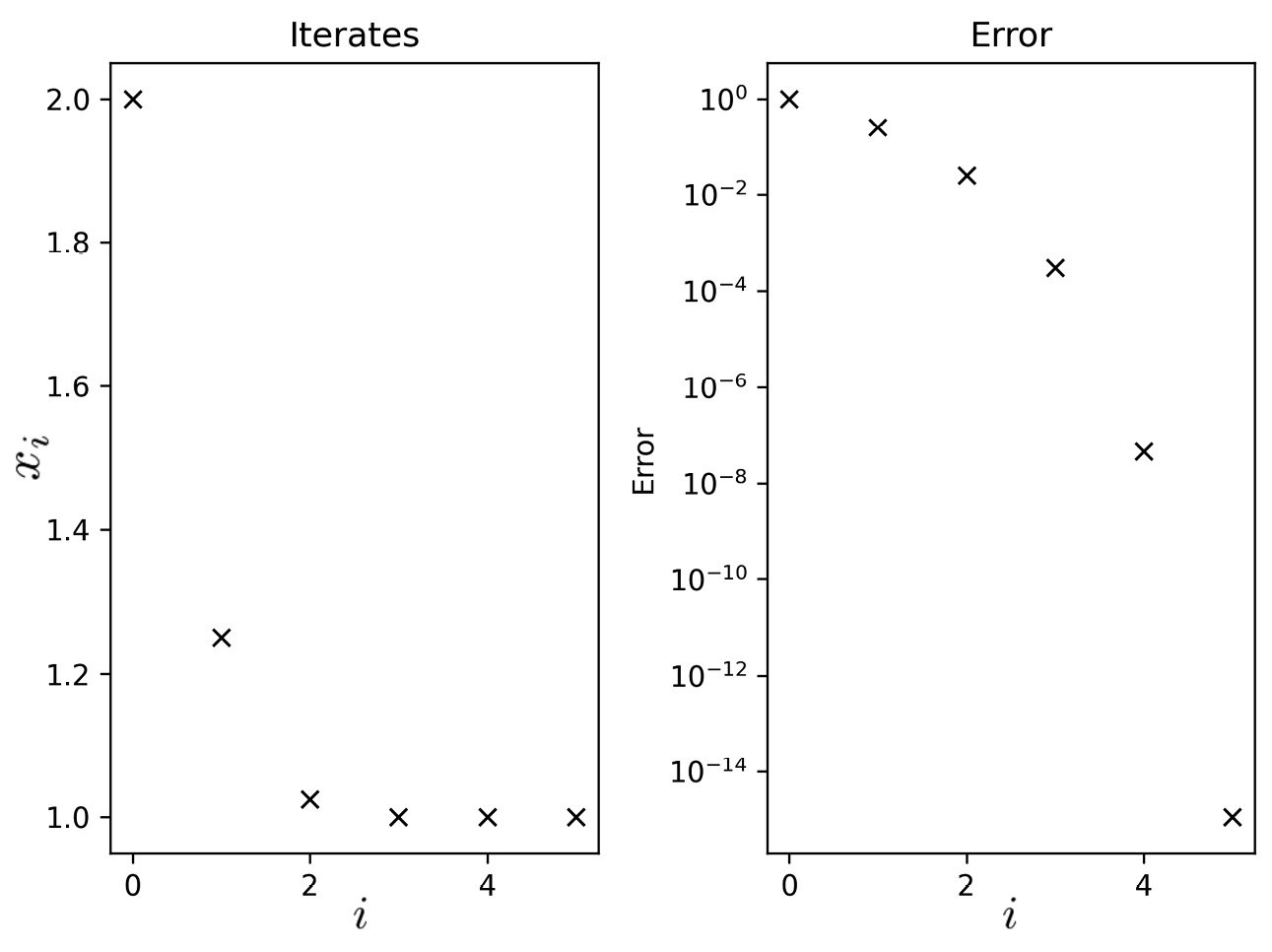
Figure 2.3 - Multiple subplots on the same Matplotlib figure
The left-hand side plots the first five iterates of Newton’s method, and the right-hand side is the approximation error plotted on a logarithmic scale.
How it works...
A Figure object in Matplotlib is simply a container for plot elements, such as Axes, of a certain size. A Figure object will usually only hold a single Axes object, which occupies the entire figure area, but it can contain any number of Axes objects in the same area. The subplots routine does several things. It first creates a new figure and then creates a grid with the specified shape in the figure area. Then, a new Axes object is added to each position of the grid. The new Figure object and one or more Axes objects are then returned to the user. If a single subplot is requested (one row and one column, with no arguments) then a plain Axes object is returned. If a single row or column is requested (with more than one column or row, respectively), then a list of Axes objects is returned. If more than one row and column are requested, a list of lists, with rows represented by inner lists filled with Axes objects, will be returned. We can then use the plotting methods on each of the Axes objects to populate the figure with the desired plots.
In this recipe, we used the standard plot method for the left-hand side plot, as we have seen in previous recipes. However, for the right-hand side plot, we used a plot where the  axis had been changed to a logarithmic scale. This means that each unit on the axis represents a change of a power of 10 rather than a change of one unit so that
 0 represents  ,
, 1 represents 10, 2 represents 100, and so on. The axes labels are automatically changed to reflect this change in scale. This type of scaling is useful when the values change by an order of magnitude, such as the error in an approximation, as we use more and more iterations. We can also plot with a logarithmic scale for  only by using the
 semilogx method, or both axes on a logarithmic scale by using the loglog method.
There’s more...
There are several ways to create subplots in Matplotlib. If you have already created a Figure object, then subplots can be added using the add_subplot method of the Figure object. Alternatively, you can use the subplot routine from matplotlib.pyplot to add subplots to the current figure. If one does not yet exist, it will be created when this routine is called. The subplot routine is a convenience wrapper of the add_subplot method on the Figure object.
In the preceding example, we created two plots with differently scaled  axes. This demonstrates one of the many possible uses of subplots. Another common use is for plotting data in a matrix where columns have a common
 x label and rows have a common y label, which is especially common in multivariate statistics when investigating the correlation between various sets of data. The plt.subplots routine for creating subplots accepts the sharex and sharey keyword parameters, which allows the axes to be shared among all subplots or among a row or column. This setting affects the scale and ticks of the axes.
See also
Matplotlib supports more advanced layouts by providing the gridspec_kw keyword arguments to the subplots routine. See the documentation for matplotlib.gridspec for more information.


