The good news about spreadsheet accessibility is that a few minor changes to how you work can have a significant impact on both users that require assistive technology and those that don’t. Keeping accessibility top of mind makes spreadsheets easier for everyone. Even better, the techniques are surprisingly simple. As you’ll see, techniques such as naming your worksheets, avoiding merged cells, limiting the use of watermarks, headers, and footers, using color conscientiously, and converting lists to Tables are huge boons to able and disabled users alike.
Assign worksheet names
Every new Excel workbook starts out with at least one worksheet, and the first sheet has a default name of Sheet1. Three ways that you can add more worksheets are as follows:
- Click New Sheet, which appears as a + to the right of the worksheet tabs in modern versions of Excel, or as a miniature worksheet tab in older versions of Excel
- Choose Home | Insert drop-down menu | Insert Sheet
- Press Shift + F11
The second sheet in a workbook has a default name of Sheet2, the third Sheet3, and so on. Many times, users focus on the content within the sheets and don’t take the time to label the worksheets themselves. As you’ll see in the Check Accessibility feature section, Microsoft flags default sheet names as an accessibility issue, plus the default names make it harder for everyone to locate specific data in a workbook. Here’s how to rename a worksheet tab:
- Use any of these three techniques:
- Double-click on the worksheet tab
- Right-click on a worksheet tab, and then choose Rename
- In Excel for Windows, press F6 to select the current worksheet tab, press Shift + F10 to display the context menu, and then type
R to choose Rename
- Type up to 31 characters and then press Enter.
Nuance
The following characters cannot be used within a worksheet tab name:
\, /, *, [, ], and ?
Excel will ignore these characters if you try to type them, just as it ignores any characters beyond the first 31 that you try to type. Most other punctuation is allowed.
Worksheet names should be as specific as possible to make it easier for users to find the data they’re looking for. You can navigate between worksheets in several ways:
- In Excel for Windows, press F6 to select the current worksheet tab and then use the left or right arrow keys to navigate to a new sheet, and then press Enter.
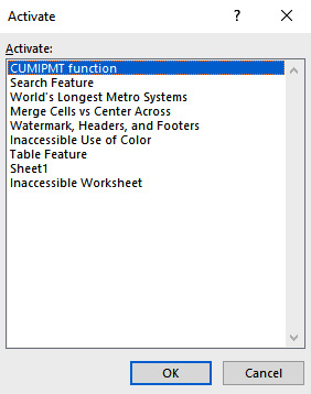
- Right-click on the navigation arrows at the bottom left-hand corner of the Excel window to display the Activate dialog box shown in Figure 1.10. Type the first letter of a sheet name to move purposefully through the list.
Figure 1.10 – Activate dialog box
Nuance
The Activate dialog box only shows visible worksheets in a workbook. Choose Home | Format | Hide & Unhide | Unhide Sheet to unhide any hidden worksheets, or right-click on any worksheet tab and choose Unhide Sheet. If Unhide Sheet is disabled, then most likely there are no hidden worksheets in the workbook. It is possible to use the Visual Basic Editor to set a worksheet to xlSheetVeryHidden, which means the worksheet cannot be unhidden through Excel’s user interface.
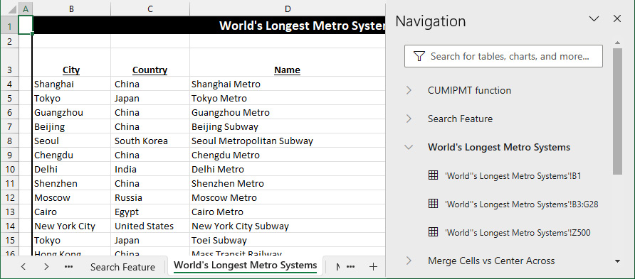
- Choose Review | Navigation in Microsoft 365 to display the Navigation pane shown in Figure 1.11:
Figure 1.11 – Navigation pane in Microsoft 365
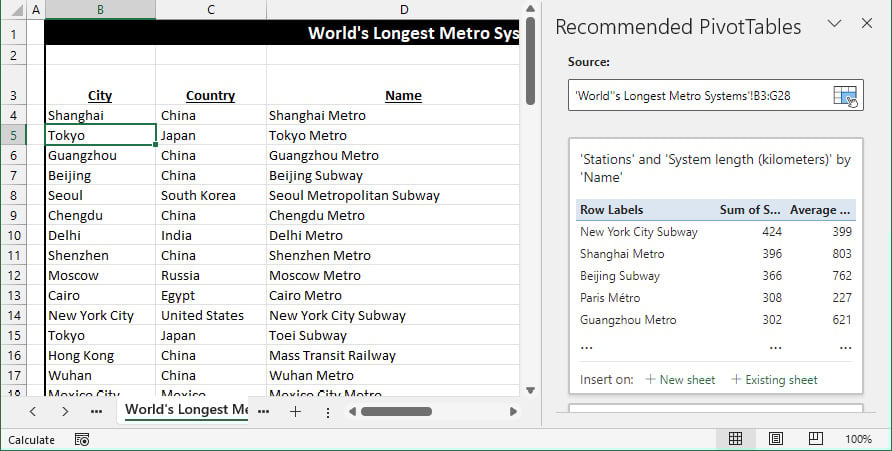
Notice that three ranges are listed on the World’s Longest Metro Systems worksheet:
- B1: The first non-blank cell on the worksheet
- B3:G28: A cluster of text, values, and/or formulas
- Z500: A random cell that I typed a tip into
The Navigation pane lists every contiguous block of non-blank cells, as well as individual non-blank cells, so you can easily determine where data appears in each worksheet.
Nuance
The Navigation task pane is only functional when you have an internet connection. As of this writing, the Navigation task pane is still in beta testing, so it may or may not be available to you as you read this, but in the worst-case scenario, it will be available in the coming months.
In Excel for Windows, press Ctrl + PgUp to move one worksheet to the left at a time or Ctrl + PgDn to move one worksheet to the right at a time, or in Excel for macOS, press Fn + ⌃ + ↓ to move one worksheet to the right at a time or Fn + ⌃ + ↑ to move one worksheet to the left.
Quirk
You cannot assign the name History to an Excel worksheet. The Track Changes feature in Excel creates a History worksheet, and so that name is a reserved word that you cannot use in Excel. You can use the word History with a space at the beginning or end, but be mindful in doing so, as users may not realize that the tab name has an extra space and could end up frustrated when trying to write formulas by typing the sheet name directly.
Let’s now explore a divisive feature that I find Excel users either absolutely love or absolutely hate.
Merge Cells feature
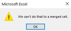
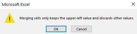
If there’s ever a reality TV series where we get to vote features out of Excel, Merge Cells is first on my list. I realize that these are fighting words for some users who rely heavily on merged cells, but from an accessibility standpoint, merged cells should be avoided whenever possible. First, merged cells can wreak havoc with assistive technology such as screen readers. Second, merged cells also wreak havoc with ordinary tasks you may try to conduct in Excel. Few things in life set my teeth on edge quite like the prompt shown in Figure 1.12. This prompt can appear even when you’re making a change that is seemingly unrelated to merged cells because the action will affect rows or columns that intersect with the merged cells:
Figure 1.12 – Merged cells error prompt
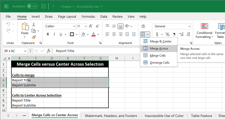
In the vein of not that you would but you could, here’s an example of how to merge cells:
- Select cells
B4:G5 on the Merge Cells vs. Center Across worksheet of this chapter’s example workbook and then choose Home | Merge & Center.
- The prompt shown in Figure 1.13 appears because we’re trying to merge more than one row of data at a time. If you click OK, Excel will merge and center cells
B4:G5 but will discard the data from row 5. You can click Undo or press Ctrl + Z (⌘ + Z) if you click through the prompt accidentally, or click Cancel to stop the merge process.
Figure 1.13 – Merged cells error prompt
- Click the Merge & Center drop-down menu and then choose Merge Across to merge cells
B4:G4 and B5:G5 separately and keep the data from each row, as shown in Figure 1.14:
Figure 1.14 – Merge Across
- Optional: Choose Home | Center to center data within the merged cells, or press
 + E in Excel for macOS.
To unmerge cells, simply select a range that includes one or more sets of merged cells and then choose Home | Merge & Center or choose Home | the Merge & Center drop-down menu | Unmerge Cells. As you’ll see in the Using the Table feature section later in this chapter, converting a range of cells to a Table automatically unmerges any cells within the list as well.
Merged cells are often used to center headings across reports, which you can easily conduct in a different manner to make the spreadsheet more accessible to users of every stripe.
Using Center Across Selection instead of merged cells
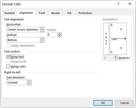
A hidden but highly effective alternative to merging cells is named Center Across Selection. This helpful feature is buried in the Format Cells dialog box. Let’s say that you want to center the headings in cells B8:B9 of Figure 1.14 across columns B:G:
- Select cells
B8:G9.
- Click the Alignment Settings button on the Home tab of the Ribbon, press Ctrl + 1 (⌘ + 1), or choose Home | Format | Format Cells.
- Activate the Alignment tab if needed.
- Choose Center Across Selection from the Horizontal list as shown in Figure 1.15, and then click OK:
Figure 1.15 – Center Across Selection
The text is now centered across columns B:G. If you change your mind about centering the text, simply select cells B8:G9 and choose Home | Align Left. Center Across Selection eliminates all of the frustrations that can arise when you merge cells but provides the same effect.
Let’s now look at aspects of Excel that can make certain information inaccessible for viewing, or even editing.
Minimizing the use of watermarks, headers, and footers
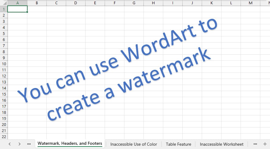
Information placed within watermarks, headers, or footers can present a particular challenge for users using assistive technology because the information doesn’t appear within the worksheet itself. However, it’s easy for any user to overlook information stored in these locations because such information is only displayed in certain contexts in Excel. Further, because there isn’t a Watermark command in Excel, it can be tricky for others to know how to remove or edit an existing watermark. A watermark is an identifier, such as a company logo, or a message, such as the words DRAFT or CONFIDENTIAL, that can be overlaid over a worksheet. One approach involves the WordArt feature:
- Choose Insert | WordArt, or Insert | Text | WordArt.
- Click on the worksheet to create a floating object and change the text as needed, as shown in Figure 1.16:
Figure 1.16 – WordArt
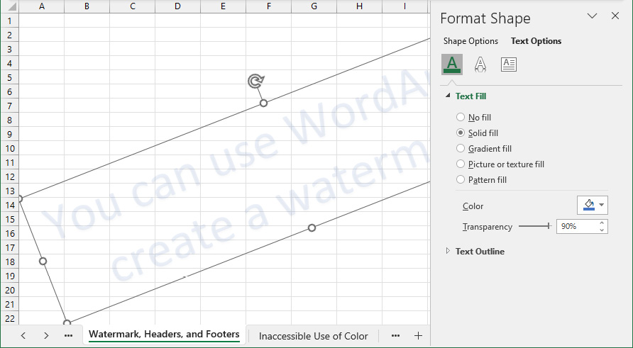
- Optional: Use the button above the text that looks like an arrow pointing in a circle, as shown in Figure 1.17, to rotate the watermark:
Figure 1.17 – Format Shape task pane and rotation arrow
- Optional: Change the transparency of the text by right-clicking on the image and choosing Format Shape | Text Options | Text Fill and then adjust the Transparency setting, as shown in Figure 1.17.
Nuance
Objects that float above the worksheet, such as WordArt and textboxes, can be tricky to format, as you have to pay attention to what is selected. If you see handles around the edge of the object, as shown in Figure 1.17, your formatting changes will affect the object as a whole. If you don’t see the handles, then most likely your formatting changes will affect some or all of the text within the object.
This sort of watermark will float above the worksheet, which means it can obscure text beneath it or confuse screen-reading technology. To remove the watermark, you can click once on the image and then press the Delete key on your keyboard.
A second approach involves placing the watermark in the header of a worksheet. The Header feature enables you to specify text that you wish to display at the top of a printed page or images that you wish to display within the body of the worksheet. The Footer feature enables you to specify text that appears at the bottom of a printed page. The challenge with headers and footers is that the user may be unaware of information stored in these sections unless they choose File | Print or View | Page Layout. Page Layout mode enables you to add a header or footer by clicking on the left, center, or right header and footer fields. A Header & Footer tab then appears in the Ribbon that contains commands that make it easy to craft headers and footers. Choose View | Normal when you’re ready to exit Page Layout mode.
Nuance
Page Layout mode is not compatible with the View | Freeze Panes feature. An alert message will appear if you try to enter Page Layout mode on a worksheet with frozen panes. If you click OK, you will enter Page Layout mode but your worksheet panes will no longer be frozen.
Alternatively, you can use these steps to add a watermark to a header without disrupting frozen worksheet panes, as well as add text to a header or footer:
- Choose Page Layout | Print Titles.
- Click the Header/Footer tab in the Page Setup dialog box.
- Click Custom Header or Custom Footer.
Nuance
Images that you place in the Header section will appear near the top of your printout, while images that you place in the Footer section will appear near the bottom of the page. You cannot place an image in the center of the printed page in this fashion unless the image is large enough to span the entire printed page.
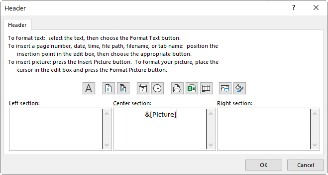
- Select a section and then click the Insert Picture button, which is the second button from the right, as shown in Figure 1.18:
Figure 1.18 – Header dialog box
- Make a choice from the Insert Pictures dialog box, which asks whether you want to choose a file from your local drive or an online resource.
- Once you select an image, a &[Picture] placeholder will appear in the section you chose, as shown in Figure 1.18.
- Optional: Click Format Picture, which is the last button on the right, to change the size of the picture. You may also wish to click on the Picture tab and change Color to Washout in the Image control section.
- Click OK as needed to close any open dialog boxes.
- Choose File | Print to display a print preview, because if you choose View | Page Layout to enter Page Layout mode, any frozen worksheet panes will become undone. You can return to the Page Setup dialog box and change the settings if needed, such as shrinking the dimensions to prevent an image from overrunning the printed page.
To remove headers or footers, choose Page Layout | Print Titles, activate the Header/Footer tab, and then choose (none) from the top of the corresponding drop-down list.
Nuance
Page Layout | Background offers a third approach for creating a watermark. The difference is that the image will repeat throughout Excel’s entire grid, and there is no way to edit the image. If you add an image in this fashion, the Background command toggles to Delete Background.
Any worksheet that has vital information in a watermark, header, or footer, such as CONFIDENTIAL or INTERNAL USE ONLY, should be considered inaccessible because assistive technology cannot access those areas of Excel. Any such information should also be repeated in cell A1, where it can be accessed by assistive technology but also be readily visible to all users of the worksheet.
Let’s now see how color can have an impact on the accessibility of your spreadsheets.
Working carefully with color
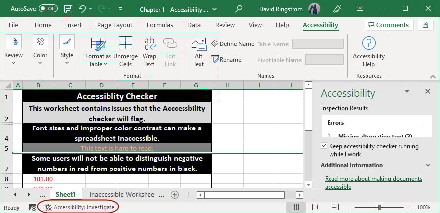
Accessibility standards call for colors to have sufficient contrast between background fill and fonts used within cells. One sure-fire way to ensure proper contrast is to use a black background with white text or light shades of gray. Black text on a white background is accessible as well. Conversely, let’s say blue text on a red background can be difficult for anyone to read, much less anyone with vision impairments or color-blindness.
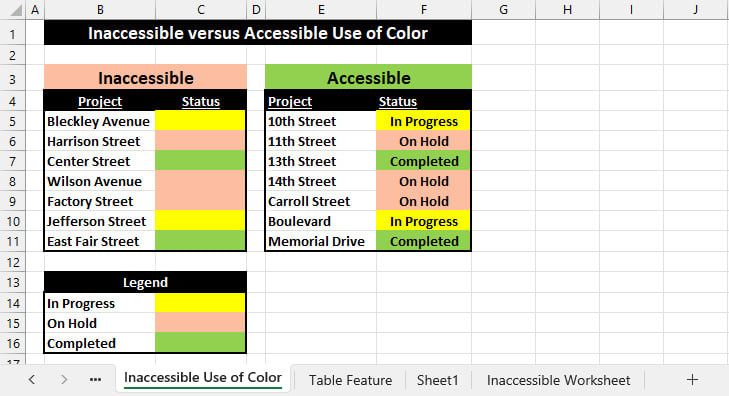
Further, standards call for any indicators in a spreadsheet that are represented by color-only to also have supportive text, as shown in Figure 1.19. As much as 8% of the world’s male population and 0.5% of the female population is color-blind. That means if you work with say nine other people, there’s a good chance at least one person may be color-blind.
Figure 1.19 – An inaccessible list versus an accessible list
The list on the left only uses color to find the status of each project, such that anyone, no matter the level of vision they have, may find themselves struggling to make sense of the data, at least at first. Conversely, the list on the right pairs the color and text together, so that all users can decide the status of each project at once. I discuss how to automate color coding based upon cell contents in Chapter 4, Conditional Formatting, along with an approach where you can combine color coding with cell icons to provide an additional means for identifying types of data.
Let’s now see how the Table feature can improve accessibility within a worksheet.
Using the Table feature
I talk extensively about the Table feature in Chapter 7, Automating Tasks with Tables, so I won’t go into much detail here, but the Table feature is one of the best ways to improve the accessibility of a worksheet. First, you cannot use merged cells within a Table; any commands or options related to merged cells are disabled when your cursor is within a Table.
Nuance
When you convert a range of cells into a Table, any merged cells within the list will be automatically unmerged because merging cells is not compatible with the Table feature.
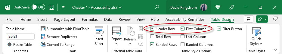
Enabling the Header Row and First Column options, as shown in Figure 1.20, can particularly improve accessibility for all:
Figure 1.20 – Table options
The Header Row allows you to place meaningful titles in the top row of a list. The titles move up into the worksheet frame when you scroll down past the first row of a Table. Filter arrows appear automatically in the Header Row to enable users to easily collapse the list down to just records of their choice. First Column makes the text in the first column bold but can also be used to help users of assistive technology know that they’re starting out in the first column rather than landing unexpectedly in the middle of a Table. Finally, assigning a meaningful name to the Table by way of Table Design | Table Name helps all users understand at once what type of data is contained within the Table. It is best to also supply a description of the data above the Header Row. As I discuss later in the book, Table Names supply an effortless way for all users of the spreadsheet to be able to jump directly to a list of data by selecting the Table Name from the Name box.
Leaving the default Table Names in place, such as Table1, Table2, Table3, and so on, quickly makes it difficult to know what data is where and cuts off the ability to move purposefully to a list of data anywhere in the workbook.
Let’s now see how you can easily find potential accessibility challenges in any workbook.
 Argentina
 Australia
 Austria
 Belgium
 Brazil
 Bulgaria
 Canada
 Chile
Chile
 Colombia
 Cyprus
 Czechia
 Denmark
 Ecuador
 Egypt
Egypt
 Estonia
 Finland
 France
 Germany
 Great Britain
 Greece
 Hungary
 India
India
 Indonesia
 Ireland
 Italy
Italy
 Japan
Japan
 Latvia
 Lithuania
 Luxembourg
 Malaysia
 Malta
Malta
 Mexico
 Netherlands
 New Zealand
 Norway
 Philippines
 Poland
 Portugal
 Romania
 Russia
 Singapore
 Slovakia
 Slovenia
 South Africa
 South Korea
 Spain
Spain
 Sweden
 Switzerland
 Taiwan
 Thailand
 Turkey
 Ukraine
 United States