In any production computer system, data constantly flows in and out and is eventually stored on storage hardware. It must be properly received, stored with the location recorded so that it can be retrieved later, retrieved as requested by the user, and sent out in the appropriate format. These tasks are handled by software commonly referred to as a relational database management system (RDBMS). SQL is the language utilized by users of an RDBMS to access and interact with a relational database.
There are many different types of RDBMS. They can be loosely categorized into two groups, commercial and open source. These RDBMSs differ slightly in the way they operate on data and even some minor parts in SQL syntax. There is an American National Standards Institute (ANSI) standard for SQL, which is largely followed by all RDBMSs. But each RDBMS may also have its own interpretations and extensions of the standard.
In this book, you will use one of the most popular open-source RDBMSs, PostgreSQL. You have installed a copy of PostgreSQL in the activities described in the preface. During that activity, you installed and enabled a PostgreSQL server application on your local machine. Your local machine's hard disk is the storage device on which data is stored. Once installation is complete, the PostgreSQL server software will be running in the backend of your computer and monitoring and handling requests from the user. Users communicate with the server software via a client tool. There are many popular client tools that you can choose from. PostgreSQL comes with two tools, a graphic user interface called pgAdmin (sometimes called pgAdmin4), and a command-line tool called psql. You used psql in the Preface. For the rest of this book, you will use pgAdmin for SQL operations.
Note
In Exercise 2.01, Running Your First SELECT Query, you will learn how to run a simple SQL query via pgAdmin in a sample database that is provided in this book, which is called the ZoomZoom database. But before the exercise, here is an explanation of how tables are organized in PostgreSQL and what tables the ZoomZoom database has.
In PostgreSQL, tables are collected in common collections in databases called schemas. One or several schemas form a database. For example, a products table can be placed in the analytics schema. Tables are usually referred to when writing queries in the format [schema].[table]. For example, a products table in the analytics schema would generally be referred to as analytics.products.
However, there is also a special schema called the public schema. This is a default schema. If you do not explicitly mention a schema when operating on a table, the database will assume the table exists in the public schema. For example, when you specify the products table without a schema name, the database will assume you are referring to the public.products table.
Here is the list of the tables in the sqlda database, as well as a brief description for each table:
closest_dealerships: Contains the distance between each customer and dealershipcountries: An empty table with columns describing countriescustomer_sales: Contains raw data in a semi-structured format of some sales recordscustomer_survey: Contains feedback with ratings from the customerscustomers: Contains detailed information for all customersdealerships: Contains detailed information for all dealershipsemails: Contains the details of emails sent to each customerproducts: Contains the products sold by ZoomZoompublic_transportation_by_zip: Contains the availability measure of public transportation in different zip codes in the United Statessales: Contains the sales records of ZoomZoom on a per customer per product basissalespeople: Contains the details of salespeople in all the dealerships top_cities_data: Contains some aggregation data for customer counts in different citiesNote
Though you may run the examples provided in this book using another RDBMS, such as MySQL, it is not guaranteed this will work as described. To make sure your results match the text, it is highly recommended that you use PostgreSQL.
Exercise 2.01: Running Your First SELECT Query
In this exercise, you will use pgAdmin to connect to a sample database called ZoomZoom on your PostgreSQL server and run a basic SQL query.
Note
You should have set up the PostgreSQL working environment while studying the preface. If you set up your PostgreSQL on a Windows or Mac, the installation wizard would have installed pgAdmin on your machine. If you set up your PostgreSQL on a Linux machine, you will need to go to the official PostgreSQL website to download and install pgAdmin, which is a separate package. Once set up, the user interface of pgAdmin is consistent across different platforms. This book will use screenshots from pgAdmin version 14 installed on a Windows machine. Your pgAdmin interface should be very similar regardless of your operating system.
Perform the following steps to complete the exercise:
- Go to
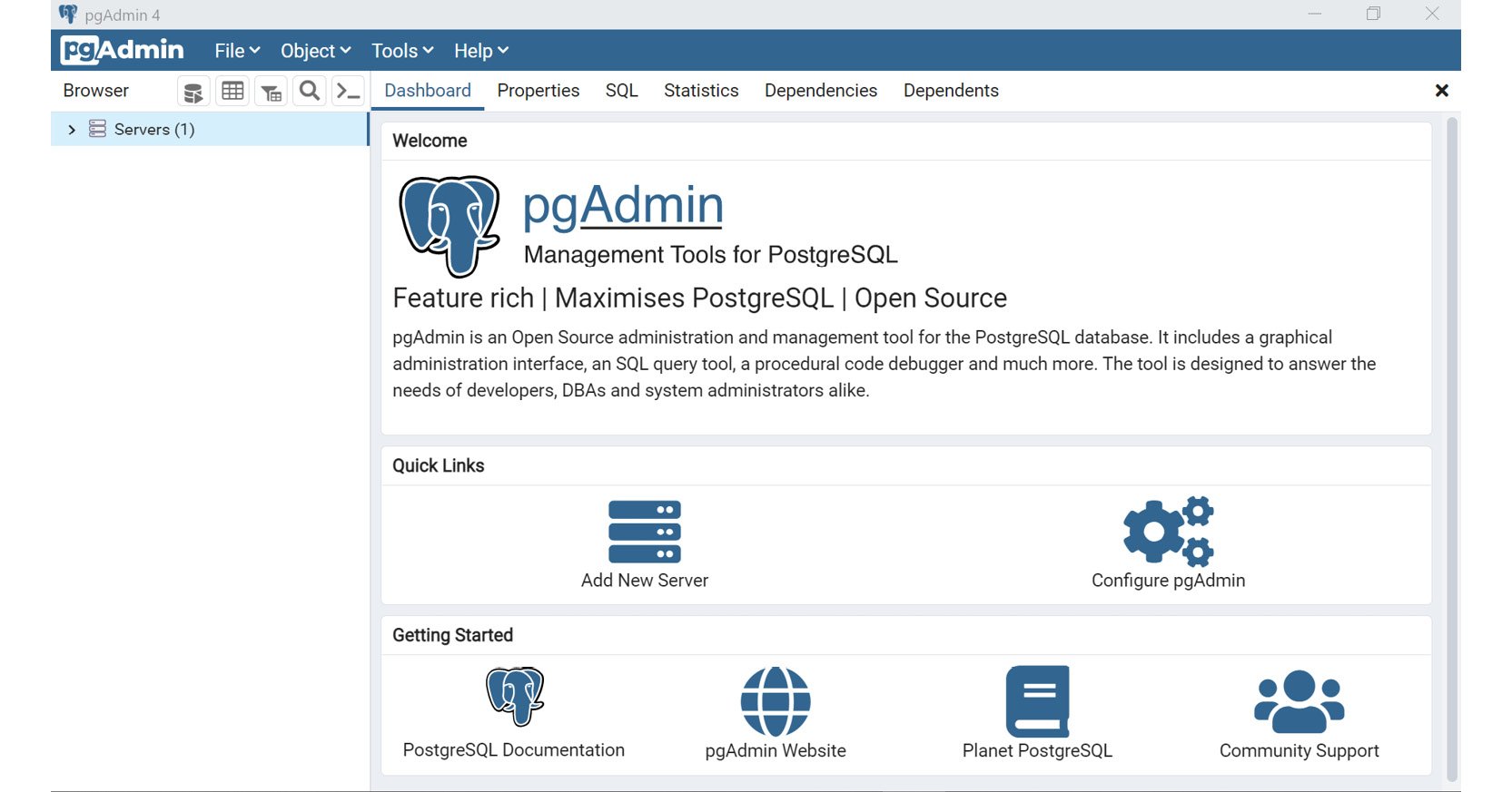
Start > PostgreSQL 14 > pgAdmin 4. The pgAdmin interface should pop up. Enter your user password when requested to do so. You will be directed to the pgAdmin Welcome page. If you are a first-time user, you will be prompted to set a password. Make sure to note down the password.
Figure 2.3: pgAdmin initial interface
- Click on the
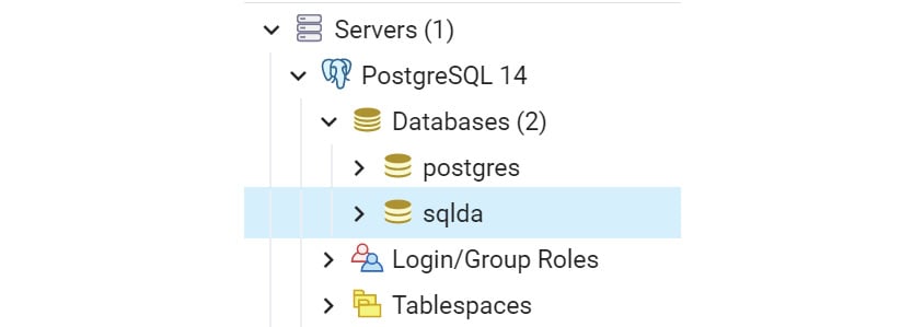
Servers in the left panel to expand its contents. You should see an entry called PostgreSQL 14. This is the PostgreSQL RDBMS installed on your machine. Click to open its content. Enter your user password when requested to do so.
Figure 2.4: Databases in PostgreSQL 14 server
You should see a Databases entry under PostgreSQL 14, which contains two databases, PostgreSQL default database postgres and a sample database called sqlda. A database is a collection of multiple tables. The sqlda database is the database that you imported in this book's preface after installing PostgreSQL.
This database has been created with a sample dataset for a fictional company called ZoomZoom, which specializes in car and electronic scooter retail. ZoomZoom sells via both the internet and its fleet of dealerships. Each dealership has a salesperson. Customers will purchase a product and optionally participate in a survey. Periodically, ZoomZoom will also send out promotional emails with meaningful subjects to customers. The dates that the email is sent, opened, and clicked, as well as the email subject and the recipient customer are recorded.
- Click the
sqlda database to open its contents. Open Schemas > public > Tables. This shows you all the tables in the public schema.
- Right-click on the
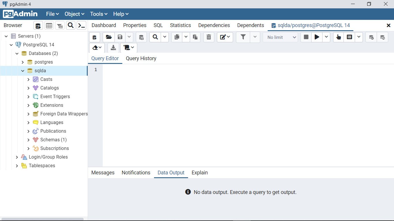
sqlda database and choose the Query Tool option to open the SQL query editor. You will see the query editor on the right side of the pgAdmin interface.
Figure 2.5: PostgreSQL SQL editor
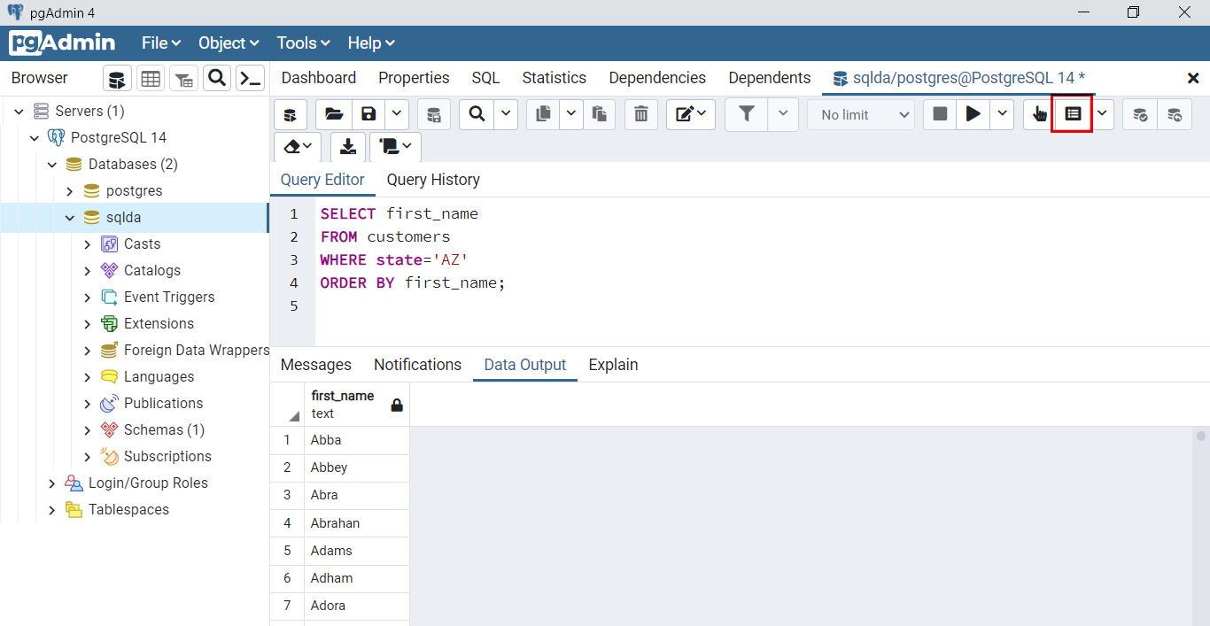
- Paste or type out the following query in the terminal. Click on the
Execute button (marked with a red circle in the following screenshot) to execute the SQL:SELECT first_name
FROM customers
WHERE state='AZ'
ORDER BY first_name;
The result of this SQL appears below the query editor:
Figure 2.6: Sample SQL and result
Note
In this screenshot, as well as many screenshots later in this book, only the first few rows are shown due to the number of rows returned exceeding the number of rows that can be displayed in this book. In addition, there is a semicolon at the end of this statement. This semicolon is not a part of the SQL statement, but it tells the PostgreSQL server that this is the end of the current statement. It is also widely used to separate several SQL statements that are grouped together and should be executed one after another.
The SQL query you just executed in this exercise is a SELECT statement. You will learn further details about this statement in the next section.
SELECT Statement
In a relational database, CRUD operations are run by running SQL statements. A SQL statement is a command that utilizes certain SQL keywords and follows certain standards to specify what result you expect from the relational database. In Exercise 2.01, Running your first SELECT query, you saw an example SQL SELECT statement. SELECT is probably the most common SQL statement; it retrieves data from a database. This operation is almost exclusively done using the SELECT keyword.
The most basic SELECT query follows this pattern:
SELECT…FROM <table_name>;
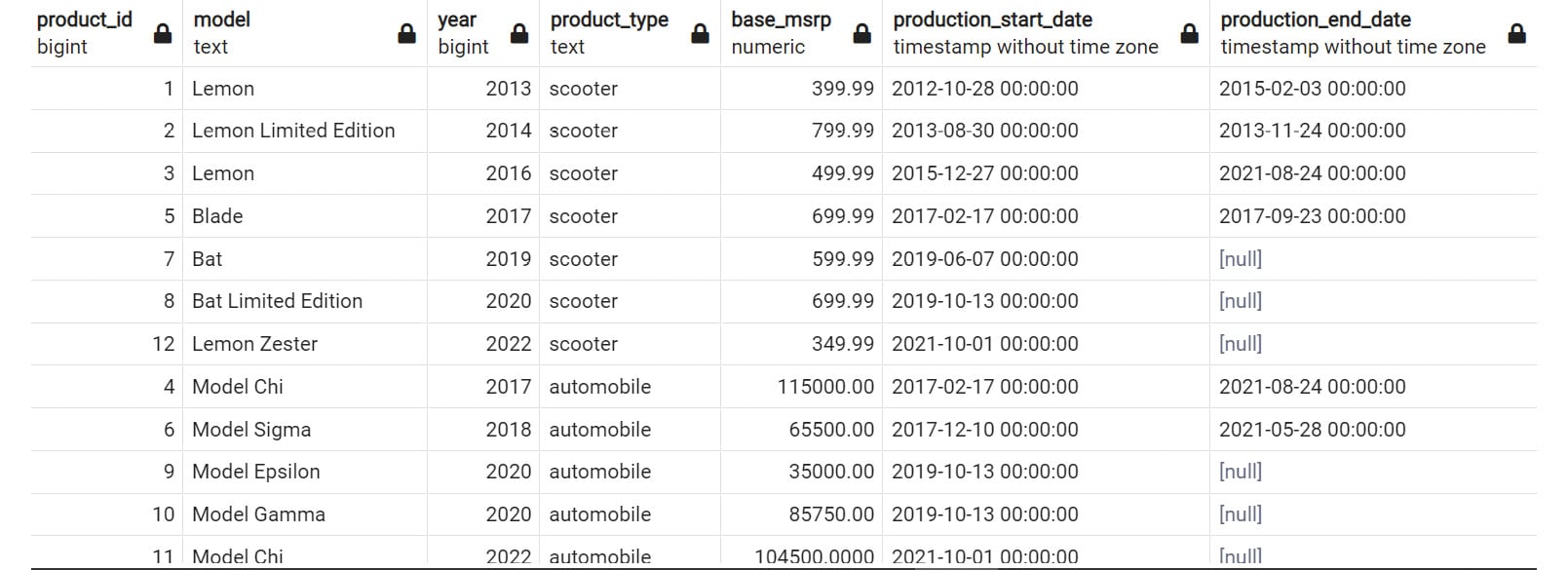
This query is a way to pull data from a single table. In its simplest form, if you want to pull all the data from the products table in the sample database, simply use this query:
SELECT * FROM products;
This query will pull all the data from a database. The output will be:
Figure 2.7: Simple SELECT statement
It is important to understand the syntax of the SELECT query in a bit more detail.
Note
In the statements used in this section, SQL keywords such as SELECT and FROM are in uppercase, while the names of tables and columns are in lowercase. SQL statements (and keywords) are case insensitive. However, when you write your own SQL, it is generally recommended to follow certain conventions on the usage of case and indentation. It will help you understand the structure and purpose of the statement.
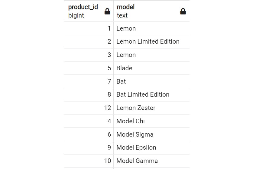
Within the SELECT clause, the * symbol is shorthand for returning all the columns from a database. The semicolon operator (;) is used to tell the computer it has reached the end of the query, much as a period is used for a normal sentence. To return only specific columns from a query, you can simply replace the asterisk (*) with the names of the columns to be returned in the order you want them to be returned. For example, if you wanted to return the product_id column followed by the model column of the products table, you would write the following query:
SELECT product_id, model FROM products;
The output will be as follows:
Figure 2.8: SELECT statement with column names
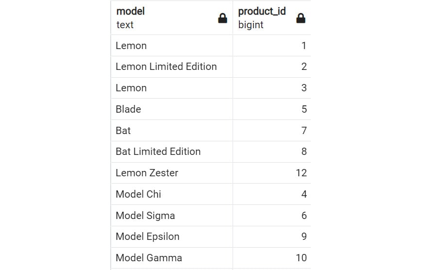
To return the model column first and the product_id column second, you would write this:
SELECT model, product_id FROM products;
The output will be the following:
Figure 2.9: SELECT statement with column names versus Figure 2.8
It is important to note that although the columns are output in the order you defined in the SELECT query, the rows will be returned in no specific order. You will learn how to output the result in a certain order in the ORDER BY section later in this chapter.
A SELECT query can be broken down into five parts:
- Operation: The first part of a query describes what is going to be displayed. In this case, the word
SELECT is followed by the names of columns combined with functions.
- Data: The next part of the query is the data, which is the
FROM keyword, followed by one or more tables connected with reserved keywords indicating which data should be scanned for filtering, selection, and calculation.
- Condition: This is a part of the query that filters the data to show only rows that meet conditions usually indicated with
WHERE.
- Grouping: This is a special clause that takes the rows of a data source and assembles them together using a key created by a
GROUP BY clause, and then calculates an output for all rows with the same value in the GROUP BY key. You will learn more about this step in Chapter 4, Aggregate Functions for Data Analysis.
- Postprocessing: This is a part of the query that takes the results of the data and formats them by sorting and limiting the data, often using keywords such as
ORDER BY and LIMIT.
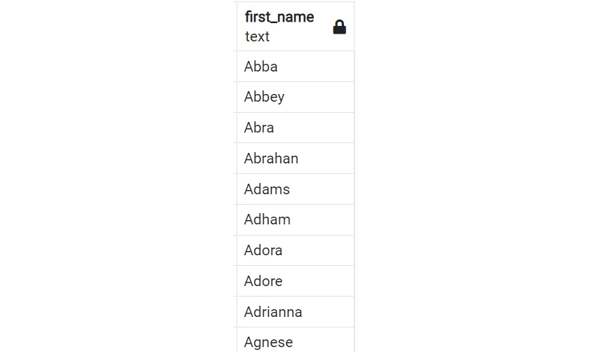
Take, for instance, the statement that you ran in Exercise 2.01, Running your first SELECT query. Suppose that, from the customers table, you wanted to retrieve the first name of all customers in the state of Arizona. You also want these names listed alphabetically. You could write the following SELECT query to retrieve this information:
SELECT first_name
FROM customers
WHERE state='AZ'
ORDER BY first_name;
The first few rows of the result look like this:
Figure 2.10: Sample SELECT statement
The operation of the query you executed in the preceding exercise follows a sequence:
- Start with the data in the
customers table.
- Filter the
customers table to where the state column equals AZ.
- Capture the
first_name column from the filtered table.
- Check the
first_name column, which is ordered alphabetically.
This demonstrates how a query can be broken down into a series of steps for the database to process. This breakdown is based on the keywords and patterns found in a SELECT query. There are many keywords that you can use while writing a SELECT query. To learn the keywords, you will start with the WHERE clause in the next section.
The WHERE Clause
The WHERE clause is a piece of conditional logic that limits the amount of data returned. You can use the WHERE clause to specify conditions based on which the SELECT statement will retrieve specific rows. In a SELECT statement, you will usually find this clause placed after the FROM clause.
The condition in the WHERE clause is generally a Boolean statement that can either be true or false for every row. In the case of numeric columns, these Boolean statements can use equals (=), greater than (>), or less than (<) operators to compare the columns against a value.
For example, say you want to see the model names of the products with the model year of 2014 from the sample dataset. You would write the following query:
SELECT model
FROM products
WHERE year=2014;
The output of this SQL is:
Figure 2.11: Simple WHERE clause
You were able to filter out the products matching a certain criterion using the WHERE clause. If you want a list of products before 2014, you could simply modify the WHERE clause to say year<2014. But what if you want to filter out rows using multiple criteria at once? Alternatively, you might also want to filter out rows that match either of two or more conditions. You can do this by adding an AND or OR clause in the queries.
The AND/OR Clause
The previous query, which outputs Figure 2.11, had only one condition. However, you might be interested in multiple conditions being met at once. For this, you need to put multiple statements together using AND or OR clauses. The AND clause helps us retrieve only the rows that match two or more conditions. The OR clause, on the other hand, retrieves rows that match one (or many) of the conditions in a set of two or more conditions.
For example, you want to return models that were not only built in 2014, but also have a Manufacturer's Suggested Retail Price (MSRP) of less than $1,000. You can write the following query:
SELECT model, year, base_msrp
FROM products
WHERE year=2014
AND base_msrp<=1000;
The result will look like this:
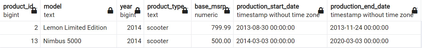
Figure 2.12: WHERE clause with AND operator
Here, you can see that the year of the product is 2014 and base_msrp is lower than $1,000. This is exactly what you are looking for.
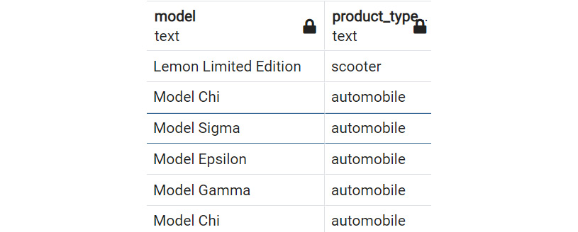
Suppose you want to return any models that were released in the year 2014 or had a product type of automobile. You would write the following query:
SELECT Model, product_type
FROM products
WHERE year=2014
OR product_type='automobile';
The result is as follows:
Figure 2.13: WHERE clause with OR operator
You already know that there is one product, Lemon Limited Edition, with a year of 2014. The rest of the products in the example have been listed with automobile as the product_type. You are seeing the combined dataset of year=2014 together with product_type='automobile'. That is exactly what the OR operator does.
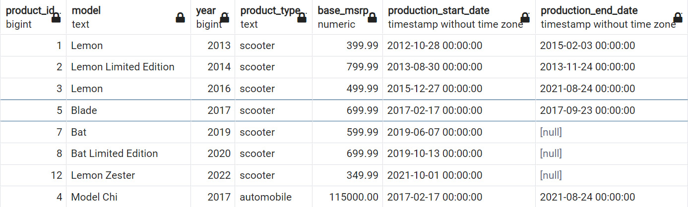
When using more than one AND or OR condition, you may need to use parentheses to separate and position pieces of logic together. This will ensure that your query works as expected and is as readable as possible. For example, if you wanted to get all products with models between the years 2016 and 2018, as well as any products that are scooters, you could write the following:
SELECT *
FROM products
WHERE year> 2016
AND year<2018
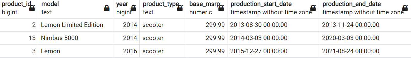
OR product_type='scooter';
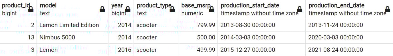
The result contains all the scooters as well as an automobile that has a year between 2016 and 2018.
Figure 2.14: WHERE clause with multiple AND/OR operators
However, to clarify the WHERE clause, it would be preferable to write the following:
SELECT *
FROM products
WHERE (year>2016 AND year<2018)
OR product_type='scooter';
You will receive the same result as above. The logic of this SQL is easier to understand. You will find that the AND and OR clauses are used quite a lot in SQL queries. However, in some scenarios, they can be tedious, especially when there are more efficient alternatives for such scenarios.
The IN/NOT IN Clause
Now that you can write queries that match multiple conditions, you also might want to refine your criteria by retrieving rows that contain (or do not contain) one or more specific values in one or more of their columns. This is where the IN and NOT IN clauses come in handy.
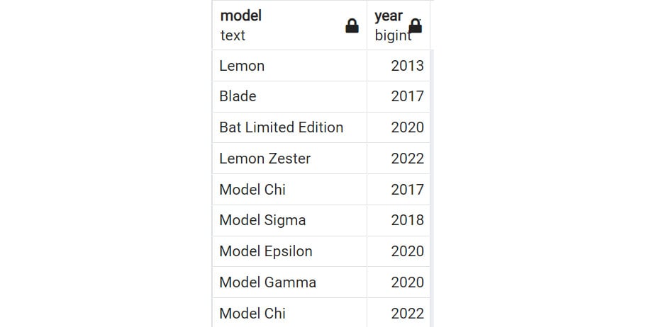
For example, you are interested in returning all models from the years 2014, 2016, or 2019. You could write a query such as this:
SELECT model, year
FROM products
WHERE year = 2014
OR year = 2016
OR year = 2019;
The result will look like the following image, showing three models from these three years:
Figure 2.15: WHERE clause with multiple OR operator
However, this is tedious to write. Using IN, you can instead write the following:
SELECT model, year
FROM products
WHERE year IN (2014, 2016, 2019);
This is much cleaner and makes it easier to understand what is going on. It will also return the same result as above.
Conversely, you can also use the NOT IN clause to return all the values that are not in a list of values. For instance, if you wanted all the products that were not produced in the years 2014, 2016, and 2019, you could write the following:
SELECT model, year
FROM products
WHERE year NOT IN (2014, 2016, 2019);
Now you see the products that are in years other than the three mentioned in the SQL statement.
Figure 2.16: WHERE clause with the NOT IN operator
In the next section, you will learn how to use the ORDER BY clause in your queries.
ORDER BY Clause
SQL queries will order rows as the database finds them if they are not given specific instructions to do otherwise. For many use cases, this is acceptable. However, you will often want to see rows in a specific order.
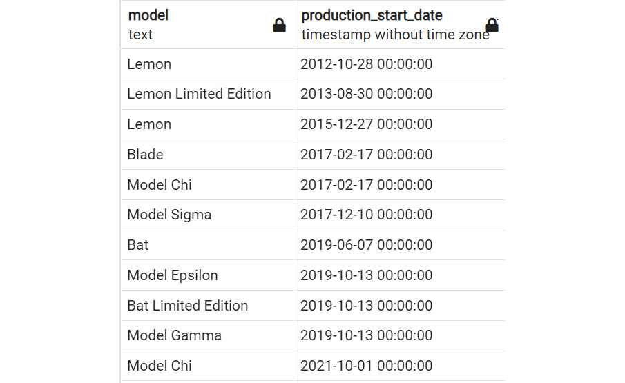
For instance, you want to see all the products listed by the date when they were first produced, from earliest to latest. The method for doing this in SQL would be using the ORDER BY clause as follows:
SELECT model, production_start_date
FROM products
ORDER BY production_start_date;
As shown in the screenshot below, the products are ordered by the production_start_date field.
Figure 2.17: SELECT statement with ORDER BY
If an order sequence is not explicitly mentioned, the rows will be returned in ascending order. Ascending order simply means the rows will be ordered from the smallest value to the highest value of the chosen column or columns. In the case of things such as text, this means arranging in alphabetical order. You can make the ascending order explicit by using the ASC keyword. For the last query, this could be achieved by writing the following:
SELECT model
FROM products
ORDER BY production_start_date ASC;
This SQL will return the same result in the same order as the SQL above.
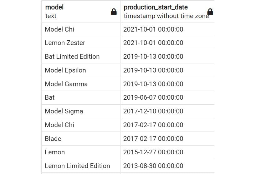
If you want to extract data in descending order, you can use the DESC keyword. If you wanted to fetch manufactured models ordered from newest to oldest, you would write the following query:
SELECT model, production_start_date
FROM products
ORDER BY production_start_date DESC;
The result will be sorted by descending order of production_start_date, latest first.
Figure 2.18: SELECT statement with ORDER BY DESC
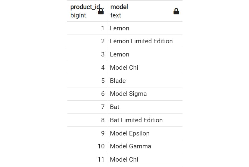
Also, instead of writing the name of the column you want to order by, you can refer to the position number of that column in the query's SELECT clause. For instance, you wanted to return all the models in the products table ordered by product ID. You could write the following:
SELECT product_id, model
FROM products
ORDER BY product_id;
The result will be like the following:
Figure 2.19: SELECT statement with numbered ORDER BY
However, because product_id is the first column in the SELECT statement, you could instead write the following:
SELECT product_id, model
FROM products
ORDER BY 1;
This SQL will return the same result as Figure 2.19.
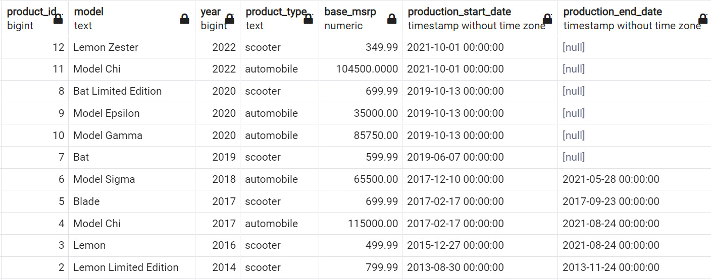
Finally, you can order by multiple columns by adding additional columns after ORDER BY, separated with commas. For instance, you want to order all the rows in the table first by the year of the model from newest to oldest, and then by the MSRP from least to greatest. You would then write the following query:
SELECT *
FROM products
ORDER BY year DESC, base_msrp ASC;
The following is the output of the preceding code:
Figure 2.20: Ordering multiple columns using ORDER BY
In the next section, you will learn about the LIMIT keyword in SQL.
The LIMIT Clause
Most tables in SQL databases tend to be quite large and, therefore, returning every single row is unnecessary. Sometimes, you may want only the first few rows. For this scenario, the LIMIT keyword comes in handy. Imagine that you wanted to only get the model of the first five products that were produced by the company. You could get this by using the following query:
SELECT model
FROM products
ORDER BY production_start_date
LIMIT 5;
The following is the output of the preceding query:
Figure 2.21: Query with LIMIT
When you are not familiar with a table or query, it is a common concern that running a SELECT statement will accidentally return many rows, which can take up a lot of time and machine bandwidth. As a common precaution, you should use the LIMIT keyword to only retrieve a small number of rows when you run the query for the first time.
IS NULL/IS NOT NULL Clause
Often, some entries in a column may be missing. This could be for a variety of reasons. Perhaps the data was not collected or not available at the time that the data was collected. Perhaps the absence of a value is representative of a certain state in the row and provides valuable information.
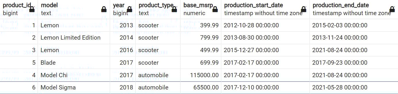
Whatever the reason, you are often interested in finding rows where the data is not filled in for a certain value. In SQL, blank values are often represented by the NULL value. For instance, in the products table, the production_end_date column having a NULL value indicates that the product is still being made. In this case, to list all products that are still being made, you can use the following query:
SELECT *
FROM products
WHERE production_end_date IS NULL;
The following is the output of the query:
Figure 2.22: Products with NULL production_end_date
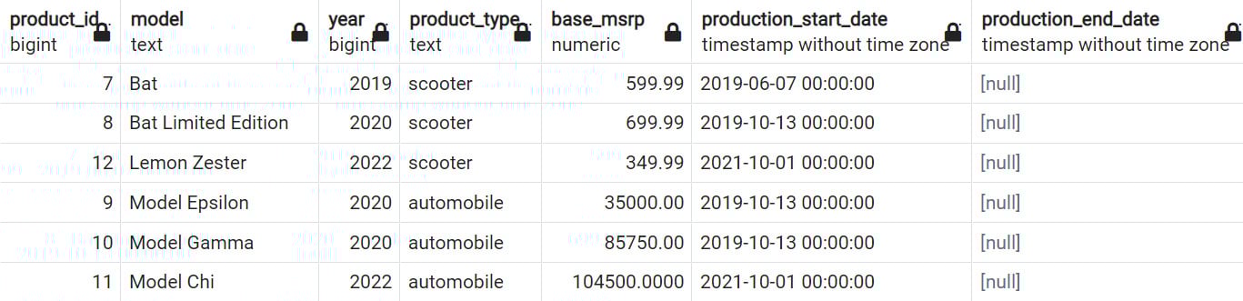
If you are only interested in products that are not being produced anymore, you can use the IS NOT NULL clause, as shown in the following query:
SELECT *
FROM products
WHERE production_end_date IS NOT NULL;
The following is the output of the code:
Figure 2.23: Products with non-NULL production_end_date
Now, you will learn how to use these new keywords in the following exercise.
Exercise 2.02: Querying the salespeople Table Using Basic Keywords in a SELECT Query
In this exercise, you will create various queries using basic keywords in a SELECT query. For instance, after a few days at your new job, you finally get access to the company database. Your boss has asked you to help a sales manager who does not know SQL particularly well. The sales manager would like a couple of different lists of salespeople.
First, you need to generate a list of the first 10 salespersons hired by dealership 17, that is, the salespersons with oldest hire_date, ordered by hiring date, with the oldest first. Second, you need to get all salespeople that were hired in 2021 and 2022 but have not been terminated, that is, the hire_date must be later than 2021-01-01, and terminiation_date is NULL, ordered by hire date, with the latest first. Finally, the manager wants to find a salesperson that was hired in 2021 but only remembers that their first name starts with "Nic." He has asked you to help find this person. You will use your SQL skill to help the manager to achieve these goals.
Note
For all future exercises in this book, you will be using pgAdmin 4.
Perform the following steps to complete the exercise:
- Open pgAdmin, connect to the
sqlda database, and open SQL query editor.
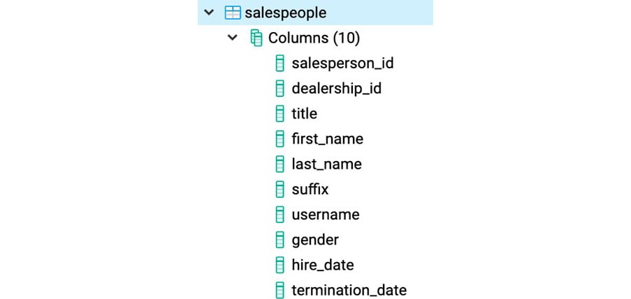
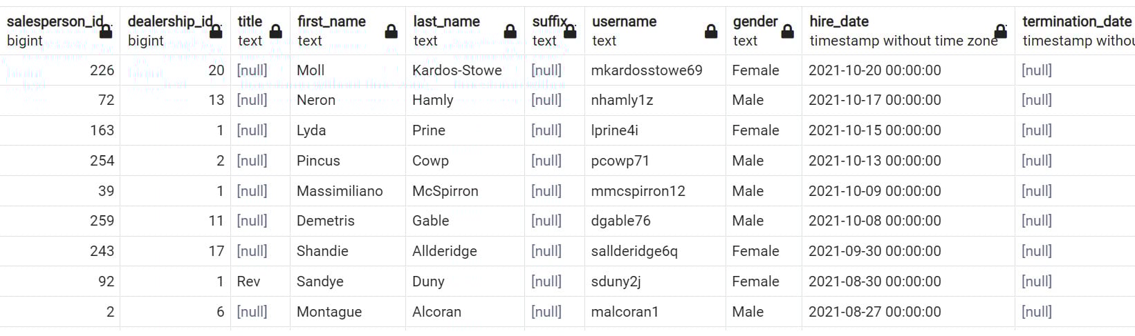
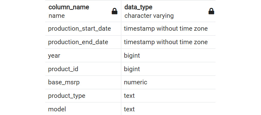
- Examine the schema for the
salespeople table from the schema drop-down list. Get familiar with the names of the columns in the following figure:
Figure 2.24: Schema of the salespeople table
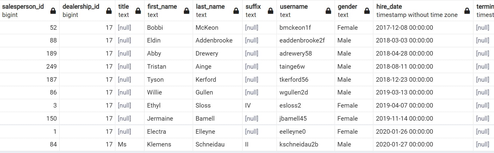
- Execute the following query to get the usernames of
salespeople from dealership_id 17, sorted by their hire_date values, and then set LIMIT to 10:SELECT *
FROM salespeople
WHERE dealership_id = 17
ORDER BY hire_date
LIMIT 10;
The following is the output of the preceding code:
Figure 2.25: Usernames of 10 earliest salespeople in dealership 17 sorted by hire date
Now you have the list of the first 10 salespersons hired by dealership 17, that is, the salespersons with the oldest hire_date, ordered by hiring date, with the oldest first.
- Now, to find all the salespeople that were hired in 2021 and 2022 but have not been terminated, that is, the
hire_date must be later than 2021-01-01, and termination_date is null, ordered by hire date, with the latest first:SELECT *
FROM salespeople
WHERE hire_date >= '2021-01-01'
AND termination_date IS NULL
ORDER BY hire_date DESC;
54 rows are returned from this SQL. The following are the first few rows of the output:
Figure 2.26: Active salespeople hired in 2021/2022 sorted by hire date latest first
- Now, find a salesperson that was hired in
2021 and whose first name starts with Nic.SELECT *
FROM salespeople
WHERE first_name LIKE 'Nic%'
AND hire_date >= '2021-01-01'
AND hire_date <= '2021-12-31';
Figure 2.27: Salespeople hired in 2021 and whose first name starts with Nic
Note
To access the source code for this specific section, please refer to https://packt.link/y2qsW.
In this exercise, you used various basic keywords in a SELECT query to help the sales manager get a list of salespeople that they needed.
Activity 2.01: Querying the customers Table Using Basic Keywords in a SELECT Query
The marketing department has decided that they want to run a series of marketing campaigns to help promote a sale. To do this, they need the email communication records for ZoomZoom customers in the state of Florida, and details of all customers in New York City. They also need the customer phone numbers with specific orders. The following are the steps to complete the activity:
- Open pgAdmin, connect to the
sqlda database, and open SQL query editor.
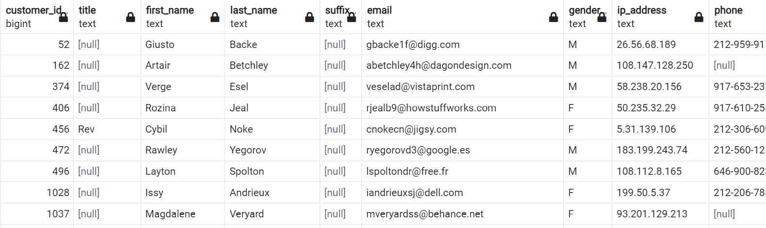
- Examine the schema for the
customers table from the schema drop-down list. Get yourself familiar with the columns in this table.
- Write a query that retrieves all emails for ZoomZoom customers in the state of Florida in alphabetical order.
- Write a query that pulls all first names, last names, and emails for ZoomZoom customers in New York City in the state of New York. They should be ordered alphabetically, with the last name followed by the first name.
- Write a query that returns all customers with a phone number ordered by the date the customer was added to the database.
The output in Figure 2.30 will help the marketing manager to carry out campaigns and promote sales.
Note
To access the source code for this specific section, please refer to https://packt.link/8bQ6n.
In this activity, you used various basic keywords in a SELECT query and helped the marketing manager to get the data they needed for the marketing campaign.
Note
The solution for this activity can be found via this link.
 Argentina
 Australia
 Austria
 Belgium
 Brazil
 Bulgaria
 Canada
 Chile
Chile
 Colombia
 Cyprus
 Czechia
 Denmark
 Ecuador
 Egypt
Egypt
 Estonia
 Finland
 France
 Germany
 Great Britain
 Greece
 Hungary
 India
India
 Indonesia
 Ireland
 Italy
Italy
 Japan
Japan
 Latvia
 Lithuania
 Luxembourg
 Malaysia
 Malta
Malta
 Mexico
 Netherlands
 New Zealand
 Norway
 Philippines
 Poland
 Portugal
 Romania
 Russia
 Singapore
 Slovakia
 Slovenia
 South Africa
 South Korea
 Spain
Spain
 Sweden
 Switzerland
 Taiwan
 Thailand
 Turkey
 Ukraine
 United States