Data. Big data. Real-time data. Data streams. Many buzzwords to describe many things, and yet they have many common properties. Mind-blowing applications can be developed from the successful application of (theoretically) simple logic – take data and produce knowledge. However, a simple-sounding task can turn out to be difficult when the amount of data needed to produce knowledge is huge (and still growing). Given the vast volumes of data produced by humanity every day, which tools should we choose to turn our simple logic into scalable solutions? That is, solutions that protect our investment in creating the data extraction logic, even in the presence of new requirements arising or changing on a daily basis, and new data processing technologies being created? This book focuses on why Apache Beam might be a good solution to these challenges, and it will guide you through the Beam learning process.

In this chapter, we will cover the following topics:

• Why Apache Beam?
• Writing your first pipeline
• Running a pipeline against streaming data
• Exploring the key properties of Unbounded data
• Measuring the event time progress inside data streams
• Assigning data to windows
• Unifying batch and streaming data processing

In this chapter, we will introduce some elementary pipelines written using Beam's Java Software Development Kit (SDK).

We will use the code located in the GitHub repository for this book: https://github.com/PacktPublishing/Building-Big-Data-Pipelines-with-Apache-Beam.

We will also need the following tools to be installed:

• Java Development Kit (JDK) 11 (possibly OpenJDK 11), with JAVA_HOME set appropriately
• Git
• Bash

  Important note

  Although it is possible to run many tools in this book using the Windows shell, we will focus on using Bash scripting only. We hope Windows users will be able to run Bash using virtualization or Windows Subsystem for Linux (or any similar technology).

First of all, we need to clone the repository:

1. To do this, we create a suitable directory, and then we run the following command:

   $ git clone https://github.com/PacktPublishing/Building-Big-Data-Pipelines-with-Apache-Beam.git

2. This will result in a directory, Building-Big-Data-Pipelines-with-Apache-Beam, being created in the working directory. We then run the following command in this newly created directory:

   $ ./mvnw clean install 

Throughout this book, the $ character will denote a Bash shell. Therefore, $ ./mvnw clean install would mean to run the ./mvnw command in the top-level directory of the git clone (that is, Building-Big-Data-Pipelines-with-Apache-Beam). By using chapter1$ ../mvnw clean install, we mean to run the specified command in the subdirectory called chapter1.

There are two basic questions we might ask when considering a new technology to learn and apply in practice:

• What problem am I struggling with that the new technology can help me solve?
• What would the costs associated with the technology be?

Every sound technology has a well-defined selling point – that is, something that justifies its existence in the presence of competing technologies. In the case of Beam, this selling point could be reduced to a single word: portability. Beam is portable on several layers:

• Beam's pipelines are portable between multiple runners (that is, a technology that executes the distributed computation described by a pipeline's author).
• Beam's data processing model is portable between various programming languages.
• Beam's data processing logic is portable between bounded and unbounded data.

Each of these points deserves a few words of explanation. By runner portability, we mean the possibility to run existing pipelines written in one of the supported programming languages (for instance, Java, Python, Go, Scala, or even SQL) against a data processing engine that can be chosen at runtime. A typical example of a runner would be Apache Flink, Apache Spark, or Google Cloud Dataflow. However, Beam is by no means limited to these; new runners are created as new technologies arise, and it's very likely that many more will be developed.

When we say Beam's data processing model is portable between various programming languages, we mean it has the ability to provide support for multiple SDKs, regardless of the language or technology used by the runner. This way, we can code Beam pipelines in the Go language, and then run these against the Apache Flink Runner, written in Java.

Last but not least, the core of Apache Beam's model is designed so that it is portable between bounded and unbounded data. Bounded data is what was historically called batch processing, while unbounded data refers to real-time processing (that is, an application crunching live data as it arrives in the system and producing a low-latency output).

Putting these pieces together, we can describe Beam as a tool that lets you deal with your big data architecture with the following vision:

Choose your preferred language, write your data processing pipeline, run this pipeline using a runner of your choice, and do all of this for both batch and real-time data at the same time.

Because everything comes at a price, you should expect to pay for flexibility like this – this price would be a somewhat bigger overhead in terms of CPU and/or memory usage. The Beam community works hard to make this overhead as small as possible, but the chances are that it will never be zero.

If all of this sounds compelling to you, then we are ready to start a journey exploring Apache Beam!

Let's jump right into writing our first pipeline. The first part of this book will focus on Beam's Java SDK. We assume that you are familiar with programming in Java and building a project using Apache Maven (or any similar tool). The following code can be found in the com.packtpub.beam.chapter1.FirstPipeline class in the chapter1 module in the GitHub repository. We would like you to go through all of the code, but we will highlight the most important parts here:

1. We need some (demo) input for our pipeline. We will read this input from the resource called lorem.txt. The code is standard Java, as follows:

   ClassLoader loader = FirstPipeline.class.getClassLoader();
   String file = loader.getResource("lorem.txt").getFile();
   List<String> lines = Files.readAllLines(
       Paths.get(file), StandardCharsets.UTF_8);

2. Next, we need to create a Pipeline object, which is a container for a Directed Acyclic Graph (DAG) that represents the data transformations needed to produce output from input data:

   Pipeline pipeline = Pipeline.create();

   Important note

   There are multiple ways to create a pipeline, and this is the simplest. We will see different approaches to pipelines in Chapter 2, Implementing, Testing, and Deploying Basic Pipelines.

3. After we create a pipeline, we can start filling it with data. In Beam, data is represented by a PCollection object. Each PCollection object (that is, parallel collection) can be imagined as a line (an edge) connecting two vertices (PTransforms, or parallel transforms) in the pipeline's DAG.
4. Therefore, the following code creates the first node in the pipeline. The node is a transform that takes raw input from the list and creates a new PCollection:

   PCollection<String> input = pipeline.apply(Create.of(lines));

   Our DAG will then look like the following diagram:

   

   Figure 1.1 – A pipeline containing a single PTransform

5. Each PTransform can have one main output and possibly multiple side output PCollections. Each PCollection has to be consumed by another PTransform or it might be excluded from the execution. As we can see, our main output (PCollection of PTransform, called Create) is not presently consumed by any PTransform. We connect PTransform to a PCollection by applying this PTransform on the PCollection. We do that by using the following code:

   PCollection<String> words = input.apply(Tokenize.of());

   This creates a new PTransform (Tokenize) and connects it to our input PCollection, as shown in the following figure:

   

   Figure 1.2 – A pipeline with two PTransforms

   We'll skip the details of how the Tokenize PTransform is implemented for now (we will return to that in Chapter 5, Using SQL for Pipeline Implementation, which describes how to structure code in general). Currently, all we have to remember is that the Tokenize PTransform takes input lines of text and splits each line into words, which produces a new PCollection that contains all of the words from all the lines of the input PCollection.

6. We finish the pipeline by adding two more PTransforms. One will produce the well-known word count example, so popular in every big data textbook. And the last one will simply print the output PCollection to standard output:

   PCollection<KV<String, Long>> result =
       words.apply(Count.perElement());
   result.apply(PrintElements.of());

   Details of both the Count PTransform (which is Beam's built-in PTransform) and PrintElements (which is a user-defined PTransform) will be discussed later. For now, if we focus on the pipeline construction process, we can see that our pipeline looks as follows:

   

   Figure 1.3 – The final word count pipeline

7. After we define this pipeline, we should run it. This is done with the following line:

   pipeline.run().waitUntilFinish();

   This causes the pipeline to be passed to a runner (configured in the pipeline; if omitted, it defaults to a runner available on Classpath). The standard default runner is the DirectRunner, which executes the pipeline in the local Java Virtual Machine (JVM) only. This runner is mostly only suitable for testing, as we will see in the next chapter.

8. We can run this pipeline by executing the following command in the code examples for the chapter1 module, which will yield the expected output on standard output:

   chapter1$ ../mvnw exec:java \
       -Dexec.mainClass=com.packtpub.beam.chapter1.FirstPipeline

   Important note

   The ordering of output is not defined and is likely to vary over multiple runs. This is to be expected and is due to the fact that the pipeline underneath is executed in multiple threads.

9. A very useful feature is that the application of PTransform to PCollection can be chained, so the preceding code can be simplified to the following:

   ClassLoader loader = ...
   FirstPipeline.class.getClassLoader();
   String file =
      loader.getResource("lorem.txt").getFile();
   List<String> lines = Files.readAllLines(
       Paths.get(file), StandardCharsets.UTF_8);
   Pipeline pipeline = Pipeline.create();
   pipeline.apply(Create.of(lines))
       .apply(Tokenize.of())
       .apply(Count.perElement())
       .apply(PrintElements.of());
   pipeline.run().waitUntilFinish();

   When used with care, this style greatly improves the readability of the code.

Now that we have written our first pipeline, let's see how to port it from a bounded data source to a streaming source!

Let's discuss how we can change this code to enable it to run against a streaming data source. We first have to define what we mean by a data stream. A data stream is a continuous flow of data without any prior information about the cardinality of the dataset. The dataset can be either finite or infinite, but we do not know which in advance. Because of this property, the streaming data is often called unbounded data, because, as opposed to bounded data, no prior bounds regarding the cardinality of the dataset can be made.

The absence of bounds is one property that makes the processing of data streams trickier (the other is that bounded data sets can be viewed as static, while unbounded data is, by definition, changing over time). We'll investigate these properties later in this chapter, and we'll see how we can leverage them to define a Beam unified model for data processing.

For now, let's imagine our pipeline is given a source, which gives one line of text at a time but does not give any signal of how many more elements there are going to be. How do we need to change our data processing logic to extract information from such a source?

1. We'll update our pipeline to use a streaming source. To do this, we need to change the way we created our input PCollection of lines coming from a List via Create PTransform to a streaming input. Beam has a utility for this called TestStream, which works as follows.

   Create a TestStream (a utility that emulates an unbounded data source). The TestStream needs a Coder (details of which will be skipped for now and will be discussed in Chapter 2, Implementing, Testing, and Deploying Basic Pipelines):

   TestStream.Builder<String> streamBuilder =
       TestStream.create(StringUtf8Coder.of());

2. Next, we fill the TestStream with data. Note that we need a timestamp for each record so that the TestStream can emulate a real stream, which should have timestamps assigned for every input element:

   Instant now = Instant.now();
   // add all lines with timestamps to the TestStream
   List<TimestampedValue<String>> timestamped =
       IntStream.range(0, lines.size())
           .mapToObj(i -> TimestampedValue.of(
              lines.get(i), now.plus(i)))
           .collect(Collectors.toList());
   for (TimestampedValue<String> value : timestamped) {
     streamBuilder = streamBuilder.addElements(value);
   }

3. Then, we will apply this to the pipeline:

   // create the unbounded PCollection from TestStream
   PCollection<String> input =
       pipeline.apply(streamBuilder.advanceWatermarkToInfinity());

   We encourage you to investigate the complete source code of the com.packtpub.beam.chapter1.MissingWindowPipeline class to make sure everything is properly understood in the preceding example.

4. Next, we run the class with the following command:

   chapter1$ ../mvnw exec:java \
       -Dexec.mainClass=\
           com.packtpub.beam.chapter1.MissingWindowPipeline

   This will result in the following exception:

   java.lang.IllegalStateException: GroupByKey cannot be applied to non-bounded PCollection in the GlobalWindow without a trigger. Use a Window.into or Window.triggering transform prior to GroupByKey.

   This is because we need a way to identify the (at least partial) completeness of the data. That is to say, the data needs (explicit or implicit) markers that define a condition that (when met) triggers a completion of a computation and outputs data from a PTransform. The computation can then continue from the values already computed or be reset to the initial state.

   There are multiple ways to define such a condition. One of them is to define time-constrained intervals called windows. A time-constrained window might be defined as data arriving within a specific time interval – for example, between 1 P.M. and 2 P.M.

5. As the exception suggests, we need to define a window to be applied to the input data stream in order to complete the definition of the pipeline. The definition of a Window is somewhat complex, and we will dive into all its parameters later in this book. But for now, we'll define the following Window:

   PCollection<String> windowed =
       words.apply(
           Window.<String>into(new GlobalWindows())
               .discardingFiredPanes()
               .triggering(AfterWatermark.pastEndOfWindow()));

   This code applies Window.into PTransform by using GlobalWindows, which is a specific Window that contains whole data (which means that it can be viewed as a Window containing the whole history and future of the universe).

   The complete code can be viewed in the com.packtpub.beam.chapter1.FirstStreamingPipeline class.

6. As usual, we can run this code using the following command:

   chapter1$ ../mvnw exec:java \
       -Dexec.mainClass=\
           com.packtpub.beam.chapter1.FirstStreamingPipeline

   This results in the same outcome as in the first example and with the same caveat – the order of output is not defined and will vary over multiple runs of the same code against the same data. The values will be absolutely deterministic, though.

Once we have successfully run our first streaming pipeline, let's dive into what exactly this streaming data is, and what to expect when we try to process it!

In the previous section, we successfully ran our sample pipeline against simulated unbounded data. We have seen that only a slight modification had to be made for the pipeline to produce output in the streaming case. Let's now dive a little deeper into understanding why this modification was necessary and how to code our pipelines to be portable from the beginning.

First of all, we need to define a notion of time. In our everyday life, time is a common thing we don't think that much about. We know what time it is at the moment, and we react to events that happen (more or less) instantly. We can plan for the future, but we cannot change the past.

When it comes to data processing, things change significantly. Let's imagine a smart home application that reads data from various sensors and acts based on the values it receives. Such an application is depicted in the following diagram:

Figure 1.4 – A simple sensor data processing application

The application reads a stream of incoming sensor data, reads the state associated with each device and/or the other settings related to the data being processed, (possibly) updates the state, and (possibly) outputs some resulting events or commands (for example, turn on a light if some condition is met).

Now, let's imagine we want to make modifications to the application logic. We add some new smart features, and we would like to know how the logic would behave if it had been fed with some historical events that we stored for a purpose like this. We cannot simply exchange the logic and push historical data through it because that would result in incorrect modifications of the state – the state might have been changed from the time we recorded our historical data. We see that we cannot mix two times – the time at which we process our data and the time at which the data originated. We usually call these two times the processing time and the event time. The first one is the time we see on our clock when an event arrives, while the other is the time at which the event occurred. A beautiful demonstration of these two times is depicted in the following table:

Figure 1.5 – Star Wars episodes' processing and event times

For those who are not familiar with the Star Wars saga, the processing time here represents the order in which the movies were released, while the event time represents the order of the episodes in the chronology of the story. By defining the event time and the processing time, we are able to explain another weird aspect of the streaming world – each data stream is inevitably unordered in terms of its event time. What do we mean by this? And why should this be inevitable?

The out-of-orderness of a data stream is shown in the following diagram:

Figure 1.6 – Unordered data stream

The circles represent data points (events), the x-axis is processing time, and the y-axis is event time. The upper-left half of the square should be empty under normal circumstances because that area represents events coming from the future – events with a higher event time than the current processing time. The rest of the data points represent events that arrive with a lower or higher delay from the time they occurred (event time). The vast majority of the delay is caused by technical reasons, such as queueing in the network stack, buffering, machine clocks being out of sync, or even outages of some parts of a distributed system. But there are also physical reasons why this happens – a vastly delayed data point is what you see if you look at the sky at night. The light coming from the stars we see with our naked eye is delayed by as much as a thousand years. Because even our physical reality works like this, the out-of-orderness is to be expected and has to be considered 'normal' in any stream processing.

So, we defined what the event and processing times are. We have a clock for measuring processing time. But what about event time? How do we measure that? Let's find out!

As we have shown, data streams are naturally unordered in terms of event time. Nevertheless, we need a way of measuring the completeness of our computation. Here is where another essential principle appears – watermarks.

A watermark is a (heuristic) algorithm that gives us an estimation of how far we have got in the event time domain. A perfect watermark gives the highest possible time (T) that guarantees no further data arrives with an event time < T. Let's demonstrate this with the following diagram:

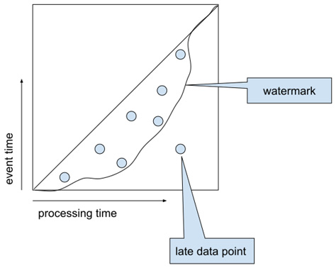
Figure 1.7 – Watermark and late data

We can see from Figure 1.7 that the watermark is a boundary that moves along with the data points, ideally leaving all of the data on its left side. All data points lying on the right side (with a processing time on the x-axis) are called late data. Such data typically requires special handling that will be described in Chapter 2, Implementing, Testing, and Deploying Basic Pipelines.

There are many ways to implement watermarks. They are typically generated at the source and propagated through the pipeline. We will discuss the details of the implementation of some watermarks in later chapters dedicated to I/O connectors. Typically, users do not have to generate watermarks themselves, although it is very useful to have a very good understanding of the concept.

States and triggers

Each computation on a data stream that takes into account more than a single isolated event needs a state. The state holds (accumulates) values derived from the so-far processed stream elements. Let's imagine we want to calculate the current number of elements in a stream. We would do that as follows:

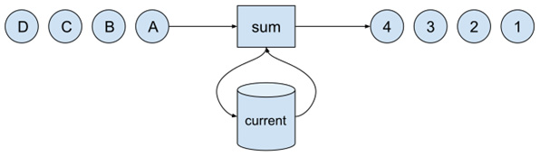
Figure 1.8 – Counting elements in a stream

The computational logic is straightforward – take the incoming element, read the current number of elements from the state, increment that number by one, store the new count into the state, and emit the current value to the output stream.

As simple as this sounds, the overall picture becomes quite complex when we consider that what we are building is an application that is supposed to run for a very long time (theoretically, forever). Such a long-running application will necessarily face disruptions caused by failing hardware, software, or necessary upgrades of the application itself. Therefore, each (sane) stream processing application has to be fault-tolerant by design.

Ensuring fault-tolerance puts specific requirements on the state and on the stream itself. Specifically, we must ensure the following:

• We must keep the state in secure, fault-tolerant storage.
• We must retain the ability to restore both the state and the stream to a defined position.

Both of these requirements dictate that every fault-tolerant stream processing engine must provide state management and state access APIs, and it must incorporate the state into its core concepts. The same holds true for Beam, and we'll dive deeper into the state concept in the following chapters.

Our element-count example raises another question: when should we output the resulting count? In the preceding example, we output the current count for each input element. This might not be adequate for every application. Other options would be to output the current value in the following ways:

• In fixed periods of processing time (for instance, every 5 seconds)
• When the watermark reaches a certain time (for instance, the output count when our watermark signals that we have processed all data up to 5 P.M.)
• When a specific condition is met in the data

Such emitting conditions are called triggers. Each of these possibilities represents one option: a processing time trigger, an event time trigger, and a data-driven trigger. Beam provides full support for processing and event time triggers and supports one data-driven trigger, which is a trigger that outputs after a specific number of elements (for example, after every 10 elements).

If you remember, we have already seen a declaration of a trigger:

PCollection<String> windowed =
    words.apply(
        Window.<String>into(new GlobalWindows())
            .discardingFiredPanes()
            .triggering(
                AfterWatermark.pastEndOfWindow()));

This is one of many event time triggers, which specifies that we want to output a result when our watermark reaches a time, and it is defined as an end-of-window. We'll dive deeper into this in later chapters when we discuss the concept of windows.

Timers

Both event time and processing time triggers require an additional stream processing concept. This concept is a timer. A timer is a tool that lets an application specify a moment in either the processing time or event time domain, and when that moment is reached, an application-defined callback hook is called. For the same reason as with states, timers also need to be fault-tolerant (that is, they have to be kept in fault-tolerant storage). Beam is purposely designed so that there is actually no way to access a watermark directly, and the only way of observing a watermark is by using event time timers. We will investigate timers in more detail in Chapter 3, Implementing Pipelines Using Stateful Processing.

We now know that a streaming data processing engine needs to manage the application's state for us, but what is the life cycle of such a state? Let's find out!

We have already touched on (but have not yet defined) the concept of a window. A window is a specific, bounded range of data within a data stream. Beam has several types of pre-defined window functions:

• Tumbling windows
• Sliding windows
• Session windows

Tumbling windows are for assigning data elements into a single window of a pre-defined length, as follows:

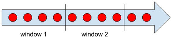
Figure 1.9 – Tumbling windows

Tumbling windows can each have exactly the same fixed length (for example, 1 hour or 1 day in what are called fixed windows), or different lengths (for example, 1 month in what are called calendar windows). The common property of tumbling windows is that the event time of each element can be assigned to exactly one window, and that these windows cover a continuous, (possibly) infinite time range, without any gaps.

Sliding windows are windows that assign data elements into multiple windows, shifted by a time period called a slide, as shown in the following figure:

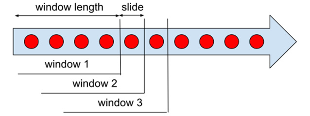
Figure 1.10 – Sliding windows

Sliding windows have the same fixed window length (for example, 1 hour) and the same fixed slide (for example, 10 minutes). A sliding window of 1 hour with a slide of 10 minutes assigns each event time into six distinct windows, each shifted by 10 minutes.

The last type of window is called a session window. This type of window is special in several ways. Unlike both previous types, session windows are key unaligned. What does that mean? Neither tumbling nor sliding windows depend on the data itself – each data element is assigned to a window (or several windows) based solely on the element's timestamp. The boundary of all the windows in the stream is exactly aligned for all the data. This is not the case for session windows. Session windows split the stream into independent sub-streams based on a user-provided key for each element in the stream. We can imagine the key as a color representing each stream element. Session windows group only elements having the same color, therefore, windows in the stream are no longer aligned on the same boundary. We can illustrate this as follows:

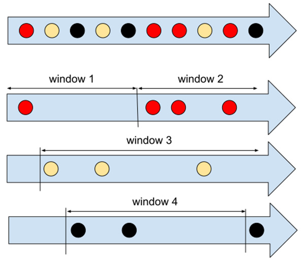
Figure 1.11 – Session windows

We can see from Figure 1.11 that different keys (types) of elements are grouped in different windows. There, one other parameter that has to be specified: a session gap duration. This duration is a timeout (in the event time) that has to elapse between the timestamps of two successive elements with the same key in order to prevent assigning them in the same window. That is to say, as long as elements for a key arrive with a frequency higher than the gap duration, all are placed in the same window. Once there is a delay of at least the gap duration, the window is closed, and another window will be created when a new element arrives. This type of window is frequently used when analyzing user sessions in web clickstreams (which is where the name session window came from).

There is one more special window type called a global window. This very special type of window assigns all data elements into a single window, regardless of their timestamp. Therefore, the window spans a complete time interval from –infinity to +infinity. This window is used as a default window before any other window is applied. We'll look into this later in this chapter.

Defining the life cycle of a state in terms of windows

Windows are actually a way of scoping a state in computation. Each state is valid within the context of a window, and each window has its own independent state.

Figure 1.12 illustrates state scoping:

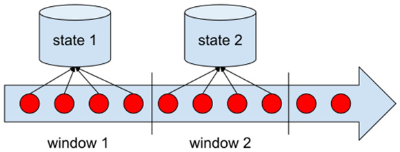
Figure 1.12 – Scoping state within windows

The scoping of states by windows brings up another crucial concept of stream processing: late data elements. One such element is shown in Figure 1.7.

We can state the problem as follows: when can we clear and discard the state that belongs to a particular window? Obviously, it is impractical to keep all states of all windows open forever, because each window carries a non-zero memory footprint, and keeping the window around for an unbounded time would cause the memory to be depleted over time. On the other hand, deleting the state right after the watermark passes the timestamp that marks the end of the window would mean we need a perfect watermark (a watermark that never produces late data). Any possible late data would mean we would produce incorrect outputs – the state would be cleared before all the data elements belonging to the respective window could be processed and therefore would have to be dropped or would produce a completely wrong outcome.

One option would be to define semantics that would require the watermark to advance only when the probability of late data is sufficiently low. We would drop all data that arrived after the watermark and pretend that we didn't see it. If the watermark produces a sufficiently low number of this late data, the error introduced by dropping the late data would be negligible. The crucial problem with this approach is that it necessarily introduces very high latency due to the out-of-orderness of stream processing. We would therefore face a latency versus correctness trade-off, when our goal ideally should be to have both high correctness and low latency.

To resolve this dilemma, stream processing engines introduce an additional concept called allowed lateness. This defines a timeout (in the event time) after which the state in a window can be cleared and all remaining data can be cleared. This option gives us the possibility to achieve the following:

• Enable the watermark heuristic to advance sufficiently quickly to not incur unnecessary latency.
• Enable an independent measure of how many states are to be kept around, even after their maximal timestamp has already passed.

We illustrate this concept in Figure 1.13, which shows a simple watermark heuristic that just shifts the processing time by a constant duration (which will define minimal latency) and a late data boundary, which shifts the watermark by an additional allowed lateness duration. This might introduce data that will be actually dropped but can now be tuned independently:

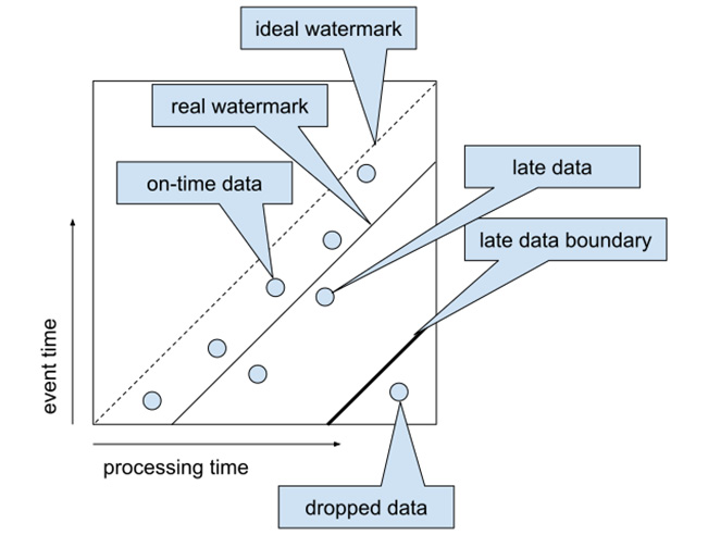
Figure 1.13 – Allowed lateness

Important note

Practical watermark implementations do not typically use a fixed shift between the watermark and processing time, but rather use statistics inferred from consumed data to produce a watermark that is non-linear in terms of the processing time.

The definition of on-time and late data brings up one last technical term that appears in the context of triggers (see the States, triggers, and timers section as a reminder). When a trigger condition is met and the trigger causes output data to be emitted downstream, three possible conditions can occur:

• The watermark has not yet reached the end timestamp of a window.
• The watermark has crossed the window end timestamp, and this is the first activation of a trigger since then.
• The watermark has passed the window end timestamp, and this is not the first activation of a trigger.

According to these three conditions, we can mark the resulting downstream data element as one of the following:

• Early: The data is emitted prior to terminating the respective window's end timestamp – this means that we output speculative partial results.
• On-time: This marks data that was calculated once the window's end timestamp was reached.
• Late: This contains any output with late data incorporated.

Beam calls data emitted as a result of trigger firings a pane and puts the information about lateness or earliness of such firing into the PaneInfo object.

Pane accumulation

When a trigger fires and causes data to be output from the current window(s) to downstream processing, there are several options that can be used with both the state associated with the window and with the resulting value itself.

After a trigger fires and data is output downstream, we have essentially two options:

• Reset the state to an empty (initial) state (discard).
• Keep the state intact (accumulate).

This concept might be a little confusing, so we'll demonstrate it with an example. Let's assume that we want to count the number of elements in a stream every minute in the processing time. In general, window functions are based on event time, so to get something that would resemble a processing time window, we can use the following:

// Window into single window and specify trigger
PCollection<String> windowed =
    words.apply(
        Window.<String>into(new GlobalWindows())
          .triggering(
           Repeatedly.forever(
              AfterProcessingTime.pastFirstElementInPane()
               .plusDelayOf(Duration.standardSeconds(1))))
          .discardingFiredPanes());

Please investigate the complete source code in the com.packtpub.beam.chapter1.ProcessingTimeWindow class.

We can run this pipeline using the following:

chapter1$ ../mvnw exec:java \
 -Dexec.mainClass=com.packtpub.beam.chapter1.ProcessingTimeWindow

Please feel free to experiment with changing discardingFiredPanes to accumulatingFiredPanes to see how the output differs. In the accumulation mode, the output contains the sum of the elements from the beginning, while in the discarding mode, it contains only increments from the last trigger firing.

Now that we have discussed all the key properties of data streams, let's see how we can use this knowledge to close the gap between batch processing and real-time stream processing!

One of the core features that Beam offers is the portability of data processing pipelines between batch and streaming processing. This began around 2004, with the famous white paper, MapReduce: Simplified Data Processing on Large Clusters. The idea behind MapReduce is quite simple: divide a complex computation into several parts, each of which consists of two functions – Map and Reduce – and apply these functions on a large scale using clusters of commodity hardware. The simplicity of the two building blocks gives rise to quite simple requirements in terms of fault tolerance, which is essential for any large distributed system.

Details of this system can be easily found online and are out of the scope of this book. We reference it here to demonstrate how and why data processing systems evolved from this moment on. The greatest benefit – massive parallel processing of data on clusters of computers that fail – is what enabled the cost-effectiveness of these large computations and finally led to the development of deep learning applications and other computationally intensive approaches.

The approach has two major drawbacks:

• Complex algorithms typically require a very difficult decomposition into Map and Reduce functions, the chaining of multiple stages, and so on.
• The latency of data processing is very high due to the fact that all data has to be reprocessed from scratch and no continuous updates are possible.

At first, both of these drawbacks were addressed by different systems. Therefore, batch systems with higher-level primitives (such as joins and groupings) came out (for example, Apache Spark), while, at the same time, different systems tailored to low-latency processing came out (for example, Apache Storm). The evolution of these systems can be illustrated as follows:

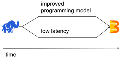
Figure 1.14 – Evolving from Apache Hadoop to Apache Beam

Apache Beam was the first model to unify both of these evolving paths into a single model, and it was targeted at both low-latency and advanced programming models. This was enabled by a simple (but very crucial) insight: batch semantics can be defined using streaming semantics (this statement is often rephrased as batch is a special case of streaming). Let's see how exactly this was achieved.

Due to the described simplicity of parallelizing a chain of MapReduce operations, practically all batch systems targeted at improving the programming model were defining high-level abstractions, which then, in turn, translated to low-level MapReduce-like operations. Therefore, we can focus on the simple MapReduce paradigm for the batch case, which works as follows:

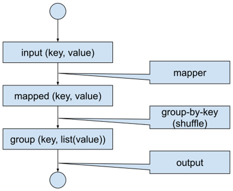
Figure 1.15 – Batch data flow

For clarity, we will briefly describe how the processing works. Each input record is fed into the Map function, producing possibly multiple key-value pairs. Each record with the same key is then grouped together and fed into the Reduce function, which (for the given key and list of values) produces final outputs.

As we have seen in this chapter, in the case of streaming semantics, there are two more things to worry about: an event time of a stream element, and a window function that assigns these elements into windows (tumbling, sliding, session). Therefore, if we extend the batch processing with the event time of each key-value pair and define a sensible default window, we get the situation depicted in Figure 1.16.

Each element is now equipped with a default timestamp (ts) and a default window:

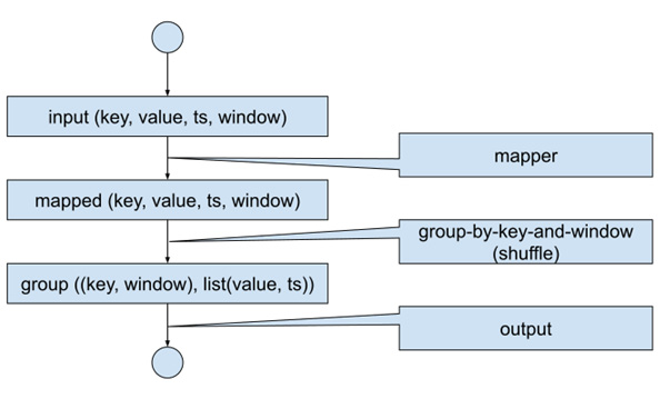
Figure 1.16 – Batch data flow with streaming semantics

We have to define sensible defaults for the timestamp and window. The timestamp can be chosen at a fixed value (typically, either the timestamp of the start of the batch computation, or –infinity), and the default window is the global window. The reason why there is no meaningful option other than to put all of the elements into a single window is that we must extend the GroupByKey operation in classical batch mode to GroupByKeyAndWindow to fulfill the streaming constraint that the state is bound to the window. In order to be able to derive the batch semantics from the streaming one, we see that the default window must assign the complete input to a single window (the global window).

Last but not least, we have to deal with how the event time moves in our streaming pipeline-running batch workflow. As we have seen, streaming processing uses watermarks to mark the progress of the event time. Batch semantics have no order in the input dataset (or in how the input data set is processed), therefore, we need to move the watermark from –infinity at the beginning and during the job to +infinity once the job completes (more exactly, when the job finishes reducing the last key).

Important note

Under special circumstances, it is possible to smoothly advance the event time watermark, even in the case of batch processing. We will learn more about this topic when we explore the stateful processing of time series data.

To sum this up, we can see that we can derive batch semantics from streaming semantics by performing the following:

• Assigning a fixed timestamp to all input key-value pairs.
• Assigning all input key-value pairs to the global window.
• Moving the watermark from –inf to +inf in one hop once all the data is processed

So, the unified approach of Beam comes from the following logic:

Code your pipeline as a streaming pipeline then run it in both a batch and streaming fashion.

There are some cases where an exception to this rule makes sense, but every time you code a batch-only pipeline in Beam, you should take one step back and think if it is really what you want.

In this chapter, we went over some of the basic theoretical concepts you will need to understand in order to keep up with the following chapters. These include the difference between processing time and event time, which is the key knowledge for being able to define the correctness of streaming computation. Processing time is mostly useful for defining the rate of the (partial) result emission via triggers, because otherwise you would always have to wait for the end of the window to get a result. We have also seen how different accumulation modes affect the output of a computation.

We have walked through the life cycle of states, as needed for aggregations. We have seen that watermarks are a systematic approach for the definition of the position in the event time and, as such, define the relationship between the event time and the processing time. We also walked through how to write your first pipeline using Beam. We'll be using these lessons as a foundation for everything we cover throughout this book.

In Chapter 2, Implementing, Testing, and Deploying Basic Pipelines, we'll be developing our understanding of pipelines even further, covering the implementation, testing, and deployment of pipelines to real distributed runners.