


 Download code from GitHub
Up and Running with Reinforcement Learning
This book will cover interesting topics in deep Reinforcement Learning (RL), including the more widely used algorithms, and will also provide TensorFlow code to solve many challenging problems using deep RL algorithms. Some basic knowledge of RL will help you pick up the advanced topics covered in this book, but the topics will be explained in a simple language that machine learning practitioners can grasp. The language of choice for this book is Python, and the deep learning framework used is TensorFlow, and we expect you to have a reasonable understanding of the two. If not, there are several Packt books that cover these topics. We will cover several different RL algorithms, such as Deep Q-Network (DQN), Deep Deterministic Policy Gradient (DDPG), Trust Region Policy Optimization (TRPO), and Proximal Policy Optimization (PPO), to name a few. Let's dive right into deep RL.
In this chapter, we will delve deep into the basic concepts of RL. We will learn the meaning of the RL jargon, the mathematical relationships between them, and also how to use them in an RL setting to train an agent. These concepts will lay the foundations for us to learn RL algorithms in later chapters, along with how to apply them to train agents. Happy learning!
Some of the main topics that will be covered in this chapter are as follows:
- Formulating the RL problem
- Understanding what an agent and an environment are
- Defining the Bellman equation
- On-policy versus off-policy learning
- Model-free versus model-based training
Why RL?
RL is a sub-field of machine learning where the learning is carried out by a trial-and-error approach. This differs from other machine learning strategies, such as the following:
- Supervised learning: Where the goal is to learn to fit a model distribution that captures a given labeled data distribution
- Unsupervised learning: Where the goal is to find inherent patterns in a given dataset, such as clustering
RL is a powerful learning approach, since you do not require labeled data, provided, of course, that you can master the learning-by-exploration approach used in RL.
While RL has been around for over three decades, the field has gained a new resurgence in recent years with the successful demonstration of the use of deep learning in RL to solve real-world tasks, wherein deep neural networks are used to make decisions. The coupling of RL with deep learning is typically referred to as deep RL, and is the main topic of discussion of this book.
Deep RL has been successfully applied by researchers to play video games, to drive cars autonomously, for industrial robots to pick up objects, for traders to make portfolio bets, by healthcare practitioners, and copious other examples. Recently, Google DeepMind built AlphaGo, a RL-based system that was able to play the game Go, and beat the champions of the game easily. OpenAI built another system to beat humans in the Dota video game. These examples demonstrate the real-world applications of RL. It is widely believed that this field has a very promising future, since you can train neural networks to make predictions without providing labeled data.
Now, let's delve into the formulation of the RL problem. We will compare how RL is similar in spirit to a child learning to walk.
Formulating the RL problem
The basic problem that is solved is training a model to make predictions of some pre-defined task without any labeled data. This is accomplished by a trial-and-error approach, akin to a baby learning to walk for the first time. A baby, curious to explore the world around them, first crawls out of their crib not knowing where to go nor what to do. Initially, they take small steps, make mistakes, keep falling on the floor, and cry. But, after many such episodes, they start to stand on their feet on their own, much to the delight of their parents. Then, with a giant leap of faith, they start to take slightly longer steps, slowly and cautiously. They still make mistakes, albeit fewer than before.
After many more such tries—and failures—they gain more confidence that enables them to take even longer steps. With time, these steps get much longer and faster, until eventually, they start to run. And that's how they grow up into a child. Was any labeled data provided to them that they used to learn to walk? No. they learned by trial and error, making mistakes along the way, learning from them, and getting better at it with infinitesimal gains made for every attempt. This is how RL works, learning by trial and error.
Building on the preceding example, here is another situation. Suppose you need to train a robot using trial and error, this is how to do it. Let the robot wander randomly in the environment initially. The good and bad actions are collected and a reward function is used to quantify them, thus, a good action performed in a state will have high rewards; on the other hand, bad actions will be penalized. This can be used as a learning signal for the robot to improve itself. After many such episodes of trial and error, the robot would have learned the best action to perform in a given state, based on the reward. This is how learning in RL works. But we will not talk about human characters for the rest of the book. The child described previously is the agent, and their surroundings are the environment in RL parlance. The agent interacts with the environment and, in the process, learns to undertake a task, for which the environment will provide a reward.
The relationship between an agent and its environment
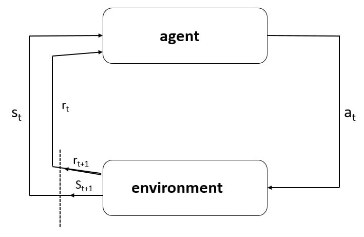
At a very basic level, RL involves an agent and an environment. An agent is an artificial intelligence entity that has certain goals, must remain vigilant about things that can come in the way of these goals, and must, at the same time, pursue the things that help in the attaining of these goals. An environment is everything that the agent can interact with. Let me explain further with an example that involves an industrial mobile robot.
For example, in a setting involving an industrial mobile robot navigating inside a factory, the robot is the agent, and the factory is the environment.
The robot has certain pre-defined goals, for example, to move goods from one side of the factory to the other without colliding with obstacles such as walls and/or other robots. The environment is the region available for the robot to navigate and includes all the places the robot can go to, including the obstacles that the robot could crash in to. So the primary task of the robot, or more precisely, the agent, is to explore the environment, understand how the actions it takes affects its rewards, be cognizant of the obstacles that can cause catastrophic crashes or failures, and then master the art of maximizing the goals and improving its performance over time.
In this process, the agent inevitably interacts with the environment, which can be good for the agent regarding certain tasks, but could be bad for the agent regarding other tasks. So, the agent must learn how the environment will respond to the actions that are taken. This is a trial-and-error learning approach, and only after numerous such trials can the agent learn how the environment will respond to its decisions.
Let's now come to understand what the state space of an agent is, and the actions that the agent performs to explore the environment.
Defining the states of the agent
In RL parlance, states represent the current situation of the agent. For example, in the previous industrial mobile robot agent case, the state at a given time instant is the location of the robot inside the factory – that is, where it is located, its orientation, or more precisely, the pose of the robot. For a robot that has joints and effectors, the state can also include the precise location of the joints and effectors in a three-dimensional space. For an autonomous car, its state can represent its speed, location on a map, distance to other obstacles, torques on its wheels, the rpm of the engine, and so on.
States are usually deduced from sensors in the real world; for instance, the measurement from odometers, LIDARs, radars, and cameras. States can be a one-dimensional vector of real numbers or integers, or two-dimensional camera images, or even higher-dimensional, for instance, three-dimensional voxels. There are really no precise limitations on states, and the state just represents the current situation of the agent.
In RL literature, states are typically represented as st, where the subscript t is used to denote the time instant corresponding to the state.
Defining the actions of the agent
The agent performs actions to explore the environment. Obtaining this action vector is the primary goal in RL. Ideally, you need to strive to obtain optimal actions.
An action is the decision an agent takes in a certain state, st. Typically, it is represented as at, where, as before, the subscript t denotes the time instant. The actions that are available to an agent depends on the problem. For instance, an agent in a maze can decide to take a step north, or south, or east, or west. These are called discrete actions, as there are a fixed number of possibilities. On the other hand, for an autonomous car, actions can be the steering angle, throttle value, brake value, and so on, which are called continuous actions as they can take real number values in a bounded range. For example, the steering angle can be 40 degrees from the north-south line, and the throttle can be 60% down, and so on.
Thus, actions at can be either discrete or continuous, depending on the problem at hand. Some RL approaches handle discrete actions, while others are suited for continuous actions.
A schematic of the agent and its interaction with the environment is shown in the following diagram:
Now that we know what an agent is, we will look at the policies that the agent learns, what value and advantage functions are, and how these quantities are used in RL.
Understanding policy, value, and advantage functions
A policy defines the guidelines for an agent's behavior at a given state. In mathematical terms, a policy is a mapping from a state of the agent to the action to be taken at that state. It is like a stimulus-response rule that the agent follows as it learns to explore the environment. In RL literature, it is usually denoted as π(at|st) – that is, it is a conditional probability distribution of taking an action at in a given state st. Policies can be deterministic, wherein the exact value of at is known at st, or can be stochastic where at is sampled from a distribution – typically this is a Gaussian distribution, but it can also be any other probability distribution.
In RL, value functions are used to define how good a state of an agent is. They are typically denoted by V(s) at state s and represent the expected long-term average rewards for being in that state. V(s) is given by the following expression where E[.] is an expectation over samples:

Note that V(s) does not care about the optimum actions that an agent needs to take at the state s. Instead, it is a measure of how good a state is. So, how can an agent figure out the most optimum action at to take in a given state st at time instant t? For this, you can also define an action-value function given by the following expression:

Note that Q(s,a) is a measure of how good is it to take action a in state s and follow the same policy thereafter. So, t is different from V(s), which is a measure of how good a given state is. We will see in the following chapters how the value function is used to train the agent under the RL setting.
The advantage function is defined as the following:
A(s,a) = Q(s,a) - V(s)
This advantage function is known to reduce the variance of policy gradients, a topic that will be discussed in depth in a later chapter.
We will now define what an episode is and its significance in an RL context.
Identifying episodes
We mentioned earlier that the agent explores the environment in numerous trials-and-errors before it can learn to maximize its goals. Each such trial from start to finish is called an episode. The start location may or may not always be from the same location. Likewise, the finish or end of the episode can be a happy or sad ending.
A happy, or good, ending can be when the agent accomplishes its pre-defined goal, which could be successfully navigating to a final destination for a mobile robot, or successfully picking up a peg and placing it in a hole for an industrial robot arm, and so on. Episodes can also have a sad ending, where the agent crashes into obstacles or gets trapped in a maze, unable to get out of it, and so on.
In many RL problems, an upper bound in the form of a fixed number of time steps is generally specified for terminating an episode, although in others, no such bound exists and the episode can last for a very long time, ending with the accomplishment of a goal or by crashing into obstacles or falling off a cliff, or something similar. The Voyager spacecraft was launched by NASA in 1977, and has traveled outside our solar system – this is an example of a system with an infinite time episode.
We will next find out what a reward function is and why we need to discount future rewards. This reward function is the key, as it is the signal for the agent to learn.
Identifying reward functions and the concept of discounted rewards
Rewards in RL are no different from real world rewards – we all receive good rewards for doing well, and bad rewards (aka penalties) for inferior performance. Reward functions are provided by the environment to guide an agent to learn as it explores the environment. Specifically, it is a measure of how well the agent is performing.
The reward function defines what the good and bad things are that can happen to the agent. For instance, a mobile robot that reaches its goal is rewarded, but is penalized for crashing into obstacles. Likewise, an industrial robot arm is rewarded for putting a peg into a hole, but is penalized for being in undesired poses that can be catastrophic by causing ruptures or crashes. Reward functions are the signal to the agent regarding what is optimum and what isn't. The agent's long-term goal is to maximize rewards and minimize penalties.
Rewards
In RL literature, rewards at a time instant t are typically denoted as Rt. Thus, the total rewards earned in an episode is given by R = r1+ r2 + ... + rt, where t is the length of the episode (which can be finite or infinite).
The concept of discounting is used in RL, where a parameter called the discount factor is used, typically represented by γ and 0 ≤ γ ≤ 1 and a power of it multiplies rt. γ = 0, making the agent myopic, and aiming only for the immediate rewards. γ = 1 makes the agent far-sighted to the point that it procrastinates the accomplishment of the final goal. Thus, a value of γ in the 0-1 range (0 and 1 exclusive) is used to ensure that the agent is neither too myopic nor too far-sighted. γ ensures that the agent prioritizes its actions to maximize the total discounted rewards, Rt, from time instant t, which is given by the following:

Since 0 ≤ γ ≤ 1, the rewards into the distant future are valued much less than the rewards that the agent can earn in the immediate future. This helps the agent to not waste time and to prioritize its actions. In practice, γ = 0.9-0.99 is typically used in most RL problems.
Learning the Markov decision process
The Markov property is widely used in RL, and it states that the environment's response at time t+1 depends only on the state and action at time t. In other words, the immediate future only depends on the present and not on the past. This is a useful property that simplifies the math considerably, and is widely used in many fields such as RL and robotics.
Consider a system that transitions from state s0 to s1 by taking an action a0 and receiving a reward r1, and thereafter from s1 to s2 taking action a1, and so on until time t. If the probability of being in a state s' at time t+1 can be represented mathematically as in the following function, then the system is said to follow the Markov property:

Note that the probability of being in state st+1 depends only on st and at and not on the past. An environment that satisfies the following state transition property and reward function as follows is said to be a Markov Decision Process (MDP):


Let's now define the very foundation of RL: the Bellman equation. This equation will help in providing an iterative solution to obtaining value functions.
Defining the Bellman equation
The Bellman equation, named after the great computer scientist and applied mathematician Richard E. Bellman, is an optimality condition associated with dynamic programming. It is widely used in RL to update the policy of an agent.
Let's define the following two quantities:


The first quantity, Ps,s', is the transition probability from state s to the new state s'. The second quantity, Rs,s', is the expected reward the agent receives from state s, taking action a, and moving to the new state s'. Note that we have assumed the MDP property, that is, the transition to state at time t+1 only depends on the state and action at time t. Stated in these terms, the Bellman equation is a recursive relationship, and is given by the following equations respectively for the value function and action-value function:


Note that the Bellman equations represent the value function V at a state, and as functions of the value function at other states; similarly for the action-value function Q.
On-policy versus off-policy learning
RL algorithms can be classified as on-policy or off-policy. We will now learn about both of these classes and how to distinguish a given RL algorithm into one or the other.
On-policy method
On-policy methods use the same policy to evaluate as was used to make the decisions on actions. On-policy algorithms generally do not have a replay buffer; the experience encountered is used to train the model in situ. The same policy that was used to move the agent from state at time t to state at time t+1, is used to evaluate if the performance was good or bad. For example, if a robot is exploring the world at a given state, if it uses its current policy to ascertain whether the actions it took in the current state were good or bad, then it is an on-policy algorithm, as the current policy is also used to evaluate its actions. SARSA, A3C, TRPO, and PPO are on-policy algorithms that we will be covering in this book.
Off-policy method
Off-policy methods, on the other hand, use different policies to make action decisions and to evaluate the performance. For instance, many off-policy algorithms use a replay buffer to store the experiences, and sample data from this buffer to train the model. During the training step, a mini-batch of experience data is randomly sampled and used to train the policy and value functions. Coming back to the previous robot example, in an off-policy setting, the robot will not use the current policy to evaluate its performance, but rather use a different policy for exploring and for evaluation. If a replay buffer is used to sample a mini-batch of experience data and then train the agent, then it is off-policy learning, as the current policy of the robot (which was used to obtain the immediate actions) is different from the policy that was used to obtain the samples in the mini-batch of experience used to train the agent (as the policy has changed from an earlier time instant when the data was collected, to the current time instant). DQN, DDQN, and DDPG are off-policy algorithms that we'll look at in later chapters of this book.
Model-free and model-based training
RL algorithms that do not learn a model of how the environment works are called model-free algorithms. By contrast, if a model of the environment is constructed, then the algorithm is called model-based. In general, if value (V) or action-value (Q) functions are used to evaluate the performance, they are called model-free algorithms as no specific model of the environment is used. On the other hand, if you build a model of how the environment transitions from one state to another or determines how many rewards the agent will receive from the environment via a model, then they are called model-based algorithms.
In model-free algorithms, as aforementioned, we do not construct a model of the environment. Thus, the agent has to take an action at a state to figure out if it is a good or a bad choice. In model-based RL, an approximate model of the environment is learned; either jointly learned along with the policy, or learned a priori. This model of the environment is used to make decisions, as well as to train the policy. We will learn more about both classes of RL algorithms in later chapters.
Algorithms covered in this book
In Chapter 2, Temporal Difference, SARSA, and Q-Learning, we will look into our first two RL algorithms: Q-learning and SARSA. Both of these algorithms are tabular-based and do not require the use of neural networks. Thus, we will code them in Python and NumPy. In Chapter 3, Deep Q-Network, we will cover DQN and use TensorFlow to code the agent for the rest of the book. We will then train it to play Atari Breakout. In Chapter 4, Double DQN, Dueling Architectures, and Rainbow, we will cover double DQN, dueling network architectures, and rainbow DQN. In Chapter 5, Deep Deterministic Policy Gradient, we will look at our first Actor-Critic RL algorithm called DDPG, learn about policy gradients, and apply them to a continuous action problem. In Chapter 6, Asynchronous Methods – A3C and A2C, we will investigate A3C, which is another RL algorithm that uses a master and several worker processes. In Chapter 7, Trust Region Policy Optimization and Proximal Policy Optimization, we will investigate two more RL algorithms: TRPO and PPO. Finally, we will apply DDPG and PPO to train an agent to drive a car autonomously in Chapter 8, Deep RL Applied to Autonomous Driving. From Chapter 3, Deep Q-Network, to Chapter 8, Deep RL Applied to Autonomous Driving, we'll use TensorFlow agents. Have fun learning RL.
Summary
In this chapter, we were introduced to the basic concepts of RL. We understood the relationship between an agent and its environment, and also learned about the MDP setting. We learned the concept of reward functions and the use of discounted rewards, as well as the idea of value and advantage functions. In addition, we saw the Bellman equation and how it is used in RL. We also learned the difference between an on-policy and an off-policy RL algorithm. Furthermore, we examined the distinction between model-free and model-based RL algorithms. All of this lays the groundwork for us to delve deeper into RL algorithms and how we can use them to train agents for a given task.
In the next chapter, we will investigate our first two RL algorithms: Q-learning and SARSA. Note that in Chapter 2, Temporal Difference, SARSA, and Q-Learning, we will be using Python-based agents as they are tabular-learning. But from Chapter 3, Deep Q-Network, onward, we will be using TensorFlow to code deep RL agents, as we will require neural networks.
Questions
- Is a replay buffer required for on-policy or off-policy RL algorithms?
- Why do we discount rewards?
- What will happen if the discount factor is γ > 1?
- Will a model-based RL agent always perform better than a model-free RL agent, since we have a model of the environment states?
- What is the difference between RL and deep RL?
Further reading
- Reinforcement Learning: An Introduction, Richard S. Sutton and Andrew G. Barto, The MIT Press, 1998
- Deep Reinforcement Learning Hands-On, Maxim Lapan, Packt Publishing, 2018: https://www.packtpub.com/big-data-and-business-intelligence/deep-reinforcement-learning-hands
