


 Download code from GitHub
Acquire and Prepare the Ingredients - Your Data
In this chapter, we will cover:
- Working with data
- Reading data from CSV files
- Reading XML data
- Reading JSON data
- Reading data from fixed-width formatted files
- Reading data from R files and R libraries
- Removing cases with missing values
- Replacing missing values with the mean
- Removing duplicate cases
- Rescaling a variable to specified min-max range
- Normalizing or standardizing data in a data frame
- Binning numerical data
- Creating dummies for categorical variables
- Handling missing data
- Correcting data
- Imputing data
- Detecting outliers
Introduction
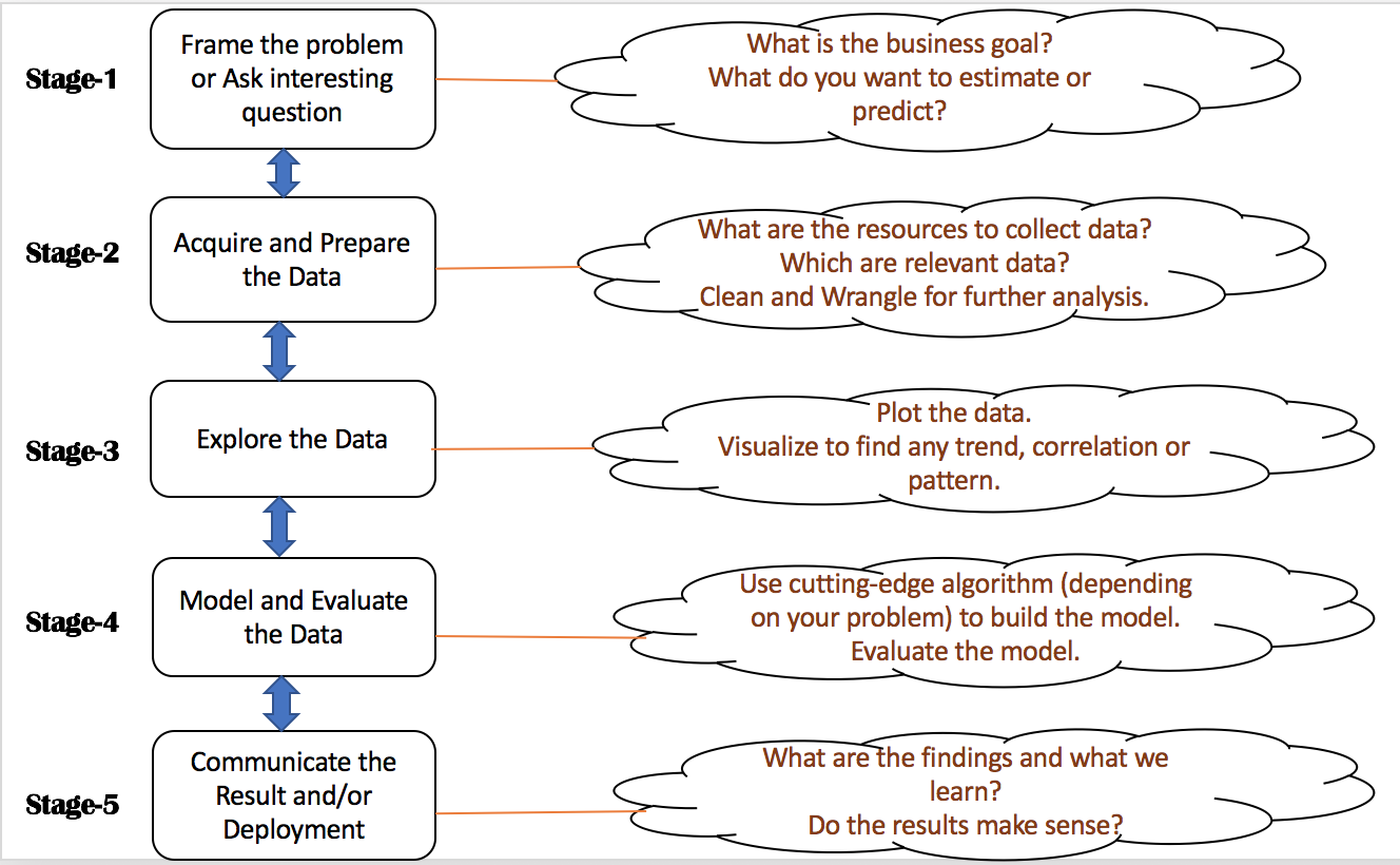
Data is everywhere and the amount of digital data that exists is growing rapidly, that is projected to grow to 180 zettabytes by 2025. Data Science is a field that tries to extract insights and meaningful information from structured and unstructured data through various stages such as asking questions, getting the data, exploring the data, modeling the data, and communicating result as shown in the following diagaram:
Data scientists or analysts often need to load or collect data from various resources having different input formats into R. Although R has its own native data format, data usually exists in text formats, such as Comma Separated Values (CSV), JavaScript Object Notation (JSON), and Extensible Markup Language (XML). This chapter provides recipes to load such data into your R system for processing.
Raw, real-world datasets are often messy with missing values, unusable format, and outliers. Very rarely can we start analyzing data immediately after loading it. Often, we will need to preprocess the data to clean, impute, wrangle, and transform it before embarking on analysis. This chapter provides recipes for some common cleaning, missing value imputation, outlier detection, and preprocessing steps.
Working with data
In the wild, datasets come in many different formats, but each computer program expects your data to be organized in a well-defined structure.
As a result, every data science project begins with the same tasks: gather the data, view the data, clean the data, correct or change the layout of the data to make it tidy, handle missing values and outliers from the data, model the data, and evaluate the data.
With R, you can do everything from collecting your data (from the web or a database) to cleaning it, transforming it, visualizing it, modelling it, and running statistical tests on it.
Reading data from CSV files
CSV formats are best used to represent sets or sequences of records in which each record has an identical list of fields. This corresponds to a single relation in a relational database, or to data (though not calculations) in a typical spreadsheet.
Getting ready
If you have not already downloaded the files for this chapter, do it now and ensure that the auto-mpg.csv file is in your R working directory.
How to do it...
Reading data from .csv files can be done using the following commands:
- Read the data from auto-mpg.csv, which includes a header row:
> auto <- read.csv("auto-mpg.csv", header=TRUE, sep = ",")
- Verify the results:
> names(auto)
How it works...
The read.csv() function creates a data frame from the data in the .csv file. If we pass header=TRUE, then the function uses the very first row to name the variables in the resulting data frame:
> names(auto)

[1] "No"           "mpg"          "cylinders"
[4] "displacement" "horsepower"   "weight"
[7] "acceleration" "model_year"   "car_name"
The header and sep parameters allow us to specify whether the .csv file has headers and the character used in the file to separate fields. The header=TRUE and sep="," parameters are the defaults for the read.csv() function; we can omit these in the code example.
There's more...
The read.csv() function is a specialized form of read.table(). The latter uses whitespace as the default field separator. We will discuss a few important optional arguments to these functions.
Handling different column delimiters
In regions where a comma is used as the decimal separator, the .csv files use ";" as the field delimiter. While dealing with such data files, use read.csv2() to load data into R.
Alternatively, you can use the read.csv("<file name>", sep=";", dec=",") command.
Use sep="t" for tab-delimited files.
Handling column headers/variable names
If your data file does not have column headers, set header=FALSE.
The auto-mpg-noheader.csv file does not include a header row. The first command in the following snippet reads this file. In this case, R assigns default variable names V1, V2, and so on.
> auto  <- read.csv("auto-mpg-noheader.csv", header=FALSE)
> head(auto,2)

  V1 V2 V3  V4 V5   V6   V7 V8                  V9
1  1 28  4 140 90 2264 15.5 71 chevrolet vega 2300
2  2 19  3  70 97 2330 13.5 72     mazda rx2 coupe
If your file does not have a header row, and you omit the header=FALSE optional argument, the read.csv() function uses the first row for variable names and ends up constructing variable names by adding X to the actual data values in the first row. Note the meaningless variable names in the following fragment:
> auto  <- read.csv("auto-mpg-noheader.csv")
> head(auto,2)

  X1 X28 X4 X140 X90 X2264 X15.5 X71 chevrolet.vega.2300
1  2  19  3   70  97  2330  13.5  72     mazda rx2 coupe
2  3  36  4  107  75  2205  14.5  82        honda accord
We can use the optional col.names argument to specify the column names. If col.names is given explicitly, the names in the header row are ignored, even if header=TRUE is specified:
> auto <- read.csv("auto-mpg-noheader.csv",     header=FALSE, col.names =       c("No", "mpg", "cyl", "dis","hp",         "wt", "acc", "year", "car_name"))

> head(auto,2)

  No mpg cyl dis hp   wt  acc year            car_name
1  1  28   4 140 90 2264 15.5   71 chevrolet vega 2300
2  2  19   3  70 97 2330 13.5   72     mazda rx2 coupe
Handling missing values
When reading data from text files, R treats blanks in numerical variables as NA (signifying missing data). By default, it reads blanks in categorical attributes just as blanks and not as NA. To treat blanks as NA for categorical and character variables, set na.strings="":
> auto <- read.csv("auto-mpg.csv", na.strings="")
If the data file uses a specified string (such as "N/A" or "NA" for example) to indicate the missing values, you can specify that string as the na.strings argument, as in na.strings= "N/A" or na.strings = "NA".
Reading strings as characters and not as factors
By default, R treats strings as factors (categorical variables). In some situations, you may want to leave them as character strings. Use stringsAsFactors=FALSE to achieve this:
> auto <- read.csv("auto-mpg.csv",stringsAsFactors=FALSE)
However, to selectively treat variables as characters, you can load the file with the defaults (that is, read all strings as factors) and then use as.character() to convert the requisite factor variables to characters.
Reading data directly from a website
If the data file is available on the web, you can load it directly into R, instead of downloading and saving it locally before loading it into R:
> dat <- read.csv("http://www.exploredata.net/ftp/WHO.csv")
Reading XML data
You may sometimes need to extract data from websites. Many providers also supply data in XML and JSON formats. In this recipe, we learn about reading XML data.
Getting ready
Make sure you have downloaded the files for this chapters and the files cd_catalog.xml and WorldPopulation-wiki.htm are in working directory of R. If the XML package is not already installed in your R environment, install the package now, as follows:
> install.packages("XML")
How to do it...
XML data can be read by following these steps:
- Load the library and initialize:
> library(XML)
> url <- "cd_catalog.xml"
- Parse the XML file and get the root node:
> xmldoc <- xmlParse(url)
> rootNode <- xmlRoot(xmldoc)
> rootNode[1]
- Extract the XML data:
> data <- xmlSApply(rootNode,function(x) xmlSApply(x, xmlValue))
- Convert the extracted data into a data frame:
> cd.catalog <- data.frame(t(data),row.names=NULL)
- Verify the results:
> cd.catalog[1:2,]
How it works...
The xmlParse function returns an object of the XMLInternalDocument class, which is a C-level internal data structure.
The xmlRoot() function gets access to the root node and its elements. Let us check the first element of the root node:
> rootNode[1]

$CD
<CD>
  <TITLE>Empire Burlesque</TITLE>
  <ARTIST>Bob Dylan</ARTIST>
  <COUNTRY>USA</COUNTRY>
  <COMPANY>Columbia</COMPANY>
  <PRICE>10.90</PRICE>
  <YEAR>1985</YEAR>
</CD>
attr(,"class")
[1] "XMLInternalNodeList" "XMLNodeList"
To extract data from the root node, we use the xmlSApply() function iteratively over all the children of the root node. The xmlSApply function returns a matrix.
To convert the preceding matrix into a data frame, we transpose the matrix using the t() function and then extract the first two rows from the cd.catalog data frame:
> cd.catalog[1:2,]
             TITLE       ARTIST COUNTRY     COMPANY PRICE YEAR
1 Empire Burlesque    Bob Dylan     USA    Columbia 10.90 1985
2  Hide your heart Bonnie Tyler      UK CBS Records  9.90 1988
There's more...
XML data can be deeply nested and hence can become complex to extract. Knowledge of XPath is helpful to access specific XML tags. R provides several functions, such as xpathSApply and getNodeSet, to locate specific elements.
Extracting HTML table data from a web page
Though it is possible to treat HTML data as a specialized form of XML, R provides specific functions to extract data from HTML tables, as follows:
> url <- "WorldPopulation-wiki.htm"
> tables <- readHTMLTable(url)
> world.pop <- tables[[6]]
The readHTMLTable() function parses the web page and returns a list of all the tables that are found on the page. For tables that have an id attribute, the function uses the id attribute as the name of that list element.
We are interested in extracting the "10 most populous countries", which is the fifth table, so we use tables[[6]].
Extracting a single HTML table from a web page
A single table can be extracted using the following command:
> table <- readHTMLTable(url,which=5)
Specify which to get data from a specific table. R returns a data frame.
Reading JSON data
Several RESTful web services return data in JSON format, in some ways simpler and more efficient than XML. This recipe shows you how to read JSON data.
Getting ready
R provides several packages to read JSON data, but we will use the jsonlite package. Install the package in your R environment, as follows:
> install.packages("jsonlite")
If you have not already downloaded the files for this chapter, do it now and ensure that the students.json files and student-courses.json files are in your R working directory.
How to do it...
Once the files are ready, load the jsonlite package and read the files as follows:
- Load the library:
> library(jsonlite)
- Load the JSON data from the files:
> dat.1 <- fromJSON("students.json")
> dat.2 <- fromJSON("student-courses.json")
- Load the JSON document from the web:
> url <- "http://finance.yahoo.com/webservice/v1/symbols/allcurrencies/quote?format=json"
> jsonDoc <- fromJSON(url)
- Extract the data into data frames:
> dat <- jsonDoc$list$resources$resource$fields
> dat.1 <- jsonDoc$list$resources$resource$fields
> dat.2 <- jsonDoc$list$resources$resource$fields
- Verify the results:
> dat[1:2,]
> dat.1[1:3,]
> dat.2[,c(1,2,4:5)]
How it works...
The jsonlite package provides two key functions: fromJSON and toJSON.
The fromJSON function can load data either directly from a file or from a web page, as the preceding steps 2 and 3 show. If you get errors in downloading content directly from the web, install and load the httr package.
Depending on the structure of the JSON document, loading the data can vary in complexity.
If given a URL, the fromJSON function returns a list object. In the preceding list, in step 4, we see how to extract the enclosed data frame.
Reading data from fixed-width formatted files
In fixed-width formatted files, columns have fixed widths; if a data element does not use up the entire allotted column width, then the element is padded with spaces to make up the specified width. To read fixed-width text files, specify the columns either by column widths or by starting positions.
Getting ready
Download the files for this chapter and store the student-fwf.txt file in your R working directory.
How to do it...
Read the fixed-width formatted file as follows:
> student <- read.fwf("student-fwf.txt", widths=c(4,15,20,15,4), col.names=c("id","name","email","major","year"))
How it works...
In the student-fwf.txt file, the first column occupies 4 character positions, the second 15, and so on. The c(4,15,20,15,4) expression specifies the widths of the 5 columns in the data file.
We can use the optional col.names argument to supply our own variable names.
There's more...
The read.fwf() function has several optional arguments that come in handy. We discuss a few of these, as follows:
Files with headers
Files with headers use the following command:
> student <- read.fwf("student-fwf-header.txt", widths=c(4,15,20,15,4), header=TRUE, sep="t",skip=2)
If header=TRUE, the first row of the file is interpreted as having the column headers. Column headers, if present, need to be separated by the specified sep argument. The sep argument only applies to the header row.
The skip argument denotes the number of lines to skip; in this recipe, the first two lines are skipped.
Excluding columns from data
To exclude a column, make the column width negative. Thus, to exclude the email column, we will specify its width as -20 and also remove the column name from the col.names vector, as follows:
> student <- read.fwf("student-fwf.txt",widths=c(4,15,-20,15,4), col.names=c("id","name","major","year"))
Reading data from R files and R libraries
During data analysis, you will create several R objects. You can save these in the native R data format and retrieve them later as needed.
Getting ready
First, create and save the R objects interactively, as shown in the following code. Make sure you have write access to the R working directory.
> customer <- c("John", "Peter", "Jane")
> orderdate <- as.Date(c('2014-10-1','2014-1-2','2014-7-6'))
> orderamount <- c(280, 100.50, 40.25)
> order <- data.frame(customer,orderdate,orderamount)
> names <- c("John", "Joan")
> save(order, names, file="test.Rdata")
> saveRDS(order,file="order.rds")
> remove(order)
After saving the preceding code, the remove() function deletes the object from the current session.
How to do it...
To be able to read data from R files and libraries, follow these steps:
- Load data from the R data files into memory:
> load("test.Rdata")
> ord <- readRDS("order.rds")
- The datasets package is loaded in the R environment by default and contains the iris and cars datasets. To load these datasets data into memory, use the following code:
> data(iris)
> data(list(cars,iris))
The first command loads only the iris dataset, and the second loads both the cars and iris datasets.
How it works...
The save() function saves the serialized version of the objects supplied as arguments along with the object name. The subsequent load() function restores the saved objects, with the same object names that they were saved with, to the global environment by default. If there are existing objects with the same names in that environment, they will be replaced without any warnings.
The saveRDS() function saves only one object. It saves the serialized version of the object and not the object name. Hence, with the readRDS() function, the saved object can be restored into a variable with a different name from when it was saved.
There's more...
The preceding recipe has shown you how to read saved R objects. We see more options in this section.
Saving all objects in a session
The following command can be used to save all objects:
> save.image(file = "all.RData")
Saving objects selectively in a session
To save objects selectively, use the following commands:
> odd <- c(1,3,5,7)
> even <- c(2,4,6,8)
> save(list=c("odd","even"),file="OddEven.Rdata")
The list argument specifies a character vector containing the names of the objects to be saved. Subsequently, loading data from the OddEven.Rdata file creates both odd and even objects. The saveRDS() function can save only one object at a time.
Attaching/detaching R data files to an environment
While loading Rdata files, if we want to be notified whether objects with the same names already exist in the environment, we can use:
> attach("order.Rdata")
The order.Rdata file contains an object named order. If an object named order already exists in the environment, we will get the following error:
The following object is masked _by_ .GlobalEnv:

    order
Listing all datasets in loaded packages
All the loaded packages can be listed using the following command:
> data()
Removing cases with missing values
Datasets come with varying amounts of missing data. When we have abundant data, we sometimes (not always) want to eliminate the cases that have missing values for one or more variables. This recipe applies when we want to eliminate cases that have any missing values, as well as when we want to selectively eliminate cases that have missing values for a specific variable alone.
Getting ready
Download the missing-data.csv file from the code files for this chapter to your R working directory. Read the data from the missing-data.csv file, while taking care to identify the string used in the input file for missing values. In our file, missing values are shown with empty strings:
> dat <- read.csv("missing-data.csv", na.strings="")
How to do it...
To get a data frame that has only the cases with no missing values for any variable, use the na.omit() function:
> dat.cleaned <- na.omit(dat)
Now dat.cleaned contains only those cases from dat that have no missing values in any of the variables.
How it works...
The na.omit() function internally uses the is.na() function, that allows us to find whether its argument is NA. When applied to a single value, it returns a Boolean value. When applied to a collection, it returns a vector:
> is.na(dat[4,2])
[1] TRUE

> is.na(dat$Income)
[1] FALSE FALSE FALSE FALSE FALSE  TRUE FALSE FALSE FALSE
[10] FALSE FALSE FALSE  TRUE FALSE FALSE FALSE FALSE FALSE
[19] FALSE FALSE FALSE FALSE FALSE FALSE FALSE FALSE FALSE
There's more...
You will sometimes need to do more than just eliminate the cases with any missing values. We discuss some options in this section.
Eliminating cases with NA for selected variables
We might sometimes want to selectively eliminate cases that have NA only for a specific variable. The example data frame has two missing values for Income. To get a data frame with only these two cases removed, use:
> dat.income.cleaned <- dat[!is.na(dat$Income),]
> nrow(dat.income.cleaned)
[1] 25
Finding cases that have no missing values
The complete.cases() function takes a data frame or table as its argument and returns a Boolean vector with TRUE for rows that have no missing values, and FALSE otherwise:
> complete.cases(dat)

 [1]  TRUE  TRUE  TRUE FALSE  TRUE FALSE  TRUE  TRUE  TRUE
[10]  TRUE  TRUE  TRUE FALSE  TRUE  TRUE  TRUE FALSE  TRUE
[19]  TRUE  TRUE  TRUE  TRUE  TRUE  TRUE  TRUE  TRUE  TRUE
Rows 4, 6, 13, and 17 have at least one missing value. Instead of using the na.omit() function, we can do the following as well:
> dat.cleaned <- dat[complete.cases(dat),]
> nrow(dat.cleaned)
[1] 23
Converting specific values to NA
Sometimes, we might know that a specific value in a data frame actually means that the data was not available. For example, in the dat data frame, a value of 0 for Income probably means that the data is missing. We can convert these to NA by a simple assignment:
> dat$Income[dat$Income==0] <- NA
Excluding NA values from computations
Many R functions return NA when some parts of the data they work on are NA. For example, computing the mean or sd on a vector with at least one NA value returns NA as the result. To remove NA from consideration, use the na.rm parameter:
> mean(dat$Income)
[1] NA

> mean(dat$Income, na.rm = TRUE)
[1] 65763.64
Replacing missing values with the mean
When you disregard cases with any missing variables, you lose useful information that the non-missing values in that case convey. You may sometimes want to impute reasonable values (those that will not skew the results of analysis very much) for the missing values.
Getting ready
Download the missing-data.csv file and store it in your R environment's working directory.
How to do it...
Read data and replace missing values:
> dat <- read.csv("missing-data.csv", na.strings = "")
> dat$Income.imp.mean <- ifelse(is.na(dat$Income),     mean(dat$Income, na.rm=TRUE), dat$Income)
After this, all the NA values for Income will be the mean value prior to imputation.
How it works...
The preceding ifelse() function returns the imputed mean value if its first argument is NA. Otherwise, it returns the first argument.
There's more...
You cannot impute the mean when a categorical variable has missing values, so you need a different approach. Even for numeric variables, we might sometimes not want to impute the mean for missing values. We discuss an often-used approach here.
Imputing random values sampled from non-missing values
If you want to impute random values sampled from the non-missing values of the variable, you can use the following two functions:
rand.impute <- function(a) {
  missing <- is.na(a)
  n.missing <- sum(missing)
  a.obs <- a[!missing]
  imputed <- a
  imputed[missing] <- sample (a.obs, n.missing, replace=TRUE)
  return (imputed)
}

random.impute.data.frame <- function(dat, cols) {
  nms <- names(dat)
  for(col in cols) {
    name <- paste(nms[col],".imputed", sep = "")
    dat[name] <- rand.impute(dat[,col])
  }
  dat
}
With these two functions in place, you can use the following to impute random values for both Income and Phone_type:
> dat <- read.csv("missing-data.csv", na.strings="")
> random.impute.data.frame(dat, c(1,2))
Removing duplicate cases
We sometimes end up with duplicate cases in our datasets and want to retain only one among them.
Getting ready
Create a sample data frame:
> salary <- c(20000, 30000, 25000, 40000, 30000, 34000, 30000)
> family.size <- c(4,3,2,2,3,4,3)
> car <- c("Luxury", "Compact", "Midsize", "Luxury",     "Compact", "Compact", "Compact")
> prospect <- data.frame(salary, family.size, car)
How to do it...
The unique() function can do the job. It takes a vector or data frame as an argument and returns an object of the same type as its argument, but with duplicates removed.
Remove duplicates to get unique values:
> prospect.cleaned <- unique(prospect)
> nrow(prospect)
[1] 7
> nrow(prospect.cleaned)
[1] 5
How it works...
The unique() function takes a vector or data frame as an argument and returns a similar object with the duplicate eliminated. It returns the non-duplicated cases as is. For repeated cases, the unique() function includes one copy in the returned result.
There's more...
Sometimes we just want to identify the duplicated values without necessarily removing them.
Identifying duplicates without deleting them
For this, use the duplicated() function:
> duplicated(prospect)
[1] FALSE FALSE FALSE FALSE  TRUE FALSE  TRUE
From the data, we know that cases 2, 5, and 7 are duplicates. Note that only cases 5 and 7 are shown as duplicates. In the first occurrence, case 2 is not flagged as a duplicate.
To list the duplicate cases, use the following code:
> prospect[duplicated(prospect), ]

  salary family.size     car
5  30000           3 Compact
7  30000           3 Compact
Rescaling a variable to specified min-max range
Distance computations play a big role in many data analytics techniques. We know that variables with higher values tend to dominate distance computations and you may want to rescale the values to be in the range of 0 - 1.
Getting ready
Install the scales package and read the data-conversion.csv file from the book's data for this chapter into your R environment's working directory:
> install.packages("scales")
> library(scales)
> students <- read.csv("data-conversion.csv")
How to do it...
To rescale the Income variable to the range [0,1], use the following code snippet:
> students$Income.rescaled <- rescale(students$Income)
How it works...
By default, the rescale() function makes the lowest value(s) zero and the highest value(s) one. It rescales all the other values proportionately. The following two expressions provide identical results:
> rescale(students$Income)
> (students$Income - min(students$Income)) /     (max(students$Income) - min(students$Income))
To rescale a different range than [0,1], use the to argument. The following snippet rescales students$Income to the range (0,100):
> rescale(students$Income, to = c(1, 100))
There's more...
When using distance-based techniques, you may need to rescale several variables. You may find it tedious to scale one variable at a time.
Rescaling many variables at once
Use the following function to rescale variables:
rescale.many <- function(dat, column.nos) {
  nms <- names(dat)
  for(col in column.nos) {
    name <- paste(nms[col],".rescaled", sep = "")
    dat[name] <- rescale(dat[,col])
  }
  cat(paste("Rescaled ", length(column.nos),      " variable(s)n"))
  dat
}
With the preceding function defined, we can do the following to rescale the first and fourth variables in the data frame:
> rescale.many(students, c(1,4))
See also
- The Normalizing or standardizing data in a data frame recipe in this chapter.
Normalizing or standardizing data in a data frame
Distance computations play a big role in many data analytics techniques. We know that variables with higher values tend to dominate distance computations and you may want to use the standardized (or z) values.
Getting ready
Download the BostonHousing.csv data file and store it in your R environment's working directory. Then read the data:
> housing <- read.csv("BostonHousing.csv")
How to do it...
To standardize all the variables in a data frame containing only numeric variables, use:
> housing.z <- scale(housing)
You can only use the scale() function on data frames that contain all numeric variables. Otherwise, you will get an error.
How it works...
When invoked in the preceding example, the scale() function computes the standard z score for each value (ignoring NAs) of each variable. That is, from each value it subtracts the mean and divides the result by the standard deviation of the associated variable.
The scale() function takes two optional arguments, center and scale, whose default values are TRUE. The following table shows the effect of these arguments:
|
Argument |
Effect |
|
center = TRUE, scale = TRUE |
Default behavior described earlier |
|
center = TRUE, scale = FALSE |
From each value, subtract the mean of the concerned variable |
|
center = FALSE, scale = TRUE |
Divide each value by the root mean square of the associated variable, where root mean square is sqrt(sum(x^2)/(n-1)) |
|
center = FALSE, scale = FALSE |
Return the original values unchanged |
There's more...
When using distance-based techniques, you may need to rescale several variables. You may find it tedious to standardize one variable at a time.
Standardizing several variables simultaneously
If you have a data frame with some numeric and some non-numeric variables, or want to standardize only some of the variables in a fully numeric data frame, then you can either handle each variable separately, which would be cumbersome, or use a function such as the following to handle a subset of variables:
scale.many <- function(dat, column.nos) {
  nms <- names(dat)
  for(col in column.nos) {
    name <- paste(nms[col],".z", sep = "")
    dat[name] <- scale(dat[,col])
  }
  cat(paste("Scaled ", length(column.nos), " variable(s)n"))
  dat
}
With this function, you can now do things like:
> housing <- read.csv("BostonHousing.csv")
> housing <- scale.many(housing, c(1,3,5:7))
This will add the z values for variables 1, 3, 5, 6, and 7, with .z appended to the original column names:
> names(housing)

[1] "CRIM"    "ZN"      "INDUS"   "CHAS"    "NOX"     "RM"
[7] "AGE"     "DIS"     "RAD"     "TAX"     "PTRATIO" "B"
[13] "LSTAT"   "MEDV"    "CRIM.z"  "INDUS.z" "NOX.z"   "RM.z"
[19] "AGE.z"
See also
Rescaling a variable to [0,1] recipe in this chapter.
Binning numerical data
Sometimes, we need to convert numerical data to categorical data or a factor. For example, Naive Bayes classification requires all variables (independent and dependent) to be categorical. In other situations, we may want to apply a classification method to a problem where the dependent variable is numeric but needs to be categorical.
Getting ready
From the code files for this chapter, store the data-conversion.csv file in the working directory of your R environment. Then read the data:
> students <- read.csv("data-conversion.csv")
How to do it...
Income is a numeric variable, and you may want to create a categorical variable from it by creating bins. Suppose you want to label incomes of $10,000 or below as Low, incomes between $10,000 and $31,000 as Medium, and the rest as High. We can do the following:
- Create a vector of break points:
> b <- c(-Inf, 10000, 31000, Inf)
- Create a vector of names for break points:
> names <- c("Low", "Medium", "High")
- Cut the vector using the break points:
> students$Income.cat <- cut(students$Income, breaks = b, labels = names)
> students

   Age State Gender Height Income Income.cat
1   23    NJ      F     61   5000        Low
2   13    NY      M     55   1000        Low
3   36    NJ      M     66   3000        Low
4   31    VA      F     64   4000        Low
5   58    NY      F     70  30000     Medium
6   29    TX      F     63  10000        Low
7   39    NJ      M     67  50000       High
8   50    VA      M     70  55000       High
9   23    TX      F     61   2000        Low
10  36    VA      M     66  20000     Medium
How it works...
The cut() function uses the ranges implied by the breaks argument to infer the bins, and names them according to the strings provided in the labels argument. In our example, the function places incomes less than or equal to 10,000 in the first bin, incomes greater than 10,000 and less than or equal to 31,000 in the second bin, and incomes greater than 31,000 in the third bin. In other words, the first number in the interval is not included but the second one is. The number of bins will be one less than the number of elements in breaks. The strings in names become the factor levels of the bins.
If we leave out names, cut() uses the numbers in the second argument to construct interval names, as you can see here:
> b <- c(-Inf, 10000, 31000, Inf)
> students$Income.cat1 <- cut(students$Income, breaks = b)
> students

   Age State Gender Height Income Income.cat     Income.cat1
1   23    NJ      F     61   5000        Low    (-Inf,1e+04]
2   13    NY      M     55   1000        Low    (-Inf,1e+04]
3   36    NJ      M     66   3000        Low    (-Inf,1e+04]
4   31    VA      F     64   4000        Low    (-Inf,1e+04]
5   58    NY      F     70  30000     Medium (1e+04,3.1e+04]
6   29    TX      F     63  10000        Low    (-Inf,1e+04]
7   39    NJ      M     67  50000       High  (3.1e+04, Inf]
8   50    VA      M     70  55000       High  (3.1e+04, Inf]
9   23    TX      F     61   2000        Low    (-Inf,1e+04]
10  36    VA      M     66  20000     Medium (1e+04,3.1e+04]
There's more...
You might not always be in a position to identify the breaks manually and may instead want to rely on R to do this automatically.
Creating a specified number of intervals automatically
Rather than determining the breaks and hence the intervals manually, as mentioned earlier, we can specify the number of bins we want, say n, and let the cut() function handle the rest automatically. In this case, cut() creates n intervals of approximately equal width, as follows:
> students$Income.cat2 <- cut(students$Income, breaks = 4, labels = c("Level1", "Level2", "Level3","Level4"))
Creating dummies for categorical variables
In situations where we have categorical variables (factors) but need to use them in analytical methods that require numbers (for example, K nearest neighbors (KNN), Linear Regression), we need to create dummy variables.
Getting ready
Read the data-conversion.csv file and store it in the working directory of your R environment. Install the dummies package. Then read the data:
> install.packages("dummies")
> library(dummies)
> students <- read.csv("data-conversion.csv")
How to do it...
Create dummies for all factors in the data frame:
> students.new <- dummy.data.frame(students, sep = ".")
> names(students.new)

[1] "Age"      "State.NJ" "State.NY" "State.TX" "State.VA"
[6] "Gender.F" "Gender.M" "Height"   "Income"
The students.new data frame now contains all the original variables and the newly added dummy variables. The dummy.data.frame() function has created dummy variables for all four levels of State and two levels of Gender factors. However, we will generally omit one of the dummy variables for State and one for Gender when we use machine learning techniques.
We can use the optional argument all = FALSE to specify that the resulting data frame should contain only the generated dummy variables and none of the original variables.
How it works...
The dummy.data.frame() function creates dummies for all the factors in the data frame supplied. Internally, it uses another dummy() function which creates dummy variables for a single factor. The dummy() function creates one new variable for every level of the factor for which we are creating dummies. It appends the variable name with the factor level name to generate names for the dummy variables. We can use the sep argument to specify the character that separates them; an empty string is the default:
> dummy(students$State, sep = ".")

      State.NJ State.NY State.TX State.VA
 [1,]        1        0        0        0
 [2,]        0        1        0        0
 [3,]        1        0        0        0
 [4,]        0        0        0        1
 [5,]        0        1        0        0
 [6,]        0        0        1        0
 [7,]        1        0        0        0
 [8,]        0        0        0        1
 [9,]        0        0        1        0
[10,]        0        0        0        1
There's more...
In situations where a data frame has several factors, and you plan on using only a subset of them, you create dummies only for the chosen subset.
Choosing which variables to create dummies for
To create a dummy only for one variable or a subset of variables, we can use the names argument to specify the column names of the variables we want dummies for:
> students.new1 <- dummy.data.frame(students, names = c("State","Gender") , sep = ".")
Handling missing data
In most real-world problems, data is likely to be incomplete because of incorrect data entry, faulty equipment, or improperly coded data. In R, missing values are represented by the symbol NA (not available) and are considered to be the first obstacle in predictive modeling. So, it's always a good idea to check for missing data in a dataset before proceeding for further predictive analysis. This recipe shows you how to handle missing data.
Getting ready
R provides three simple ways to handle missing values:
- Deleting the observations.
- Deleting the variables.
- Replacing the values with mean, median, or mode.
Install the package in your R environment as follows:
> install.packages("Hmisc")
If you have not already downloaded the files for this chapter, do it now and ensure that the housing-with-missing-value.csv file is in your R working directory.
How to do it...
Once the files are ready, load the Hmisc package and read the files as follows:
- Load the CSV data from the files:
> housing.dat <- read.csv("housing-with-missing-value.csv",header = TRUE, stringsAsFactors = FALSE)
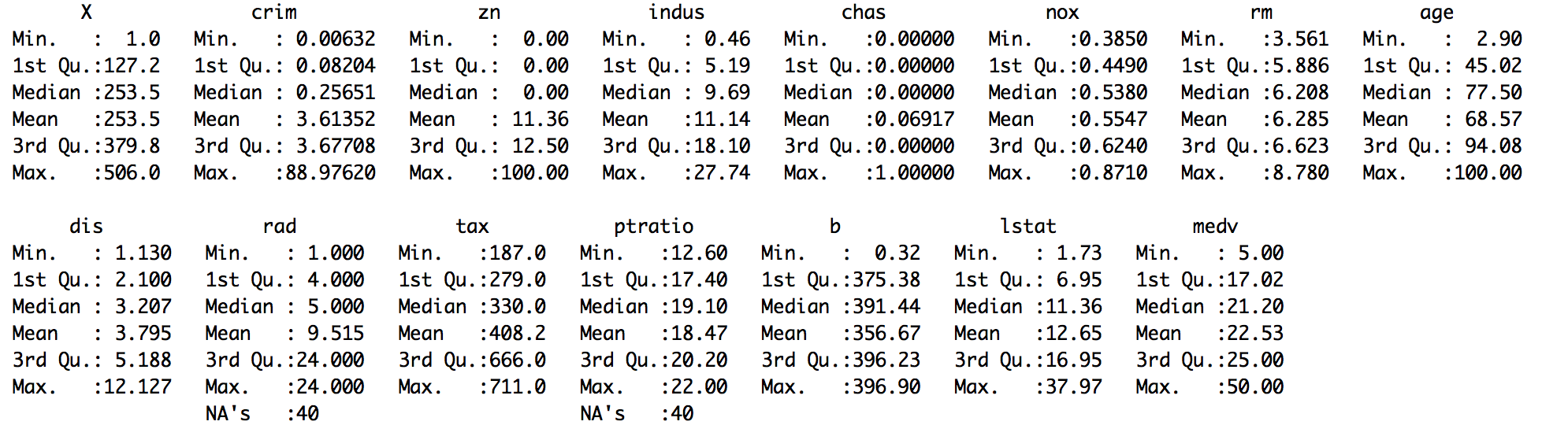
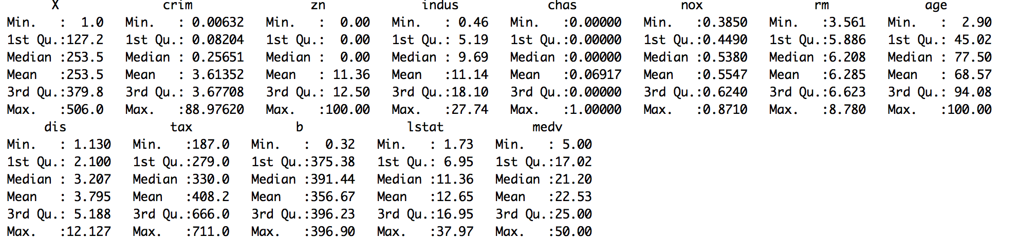
- Check summary of the dataset:
> summary(housing.dat)
The output would be as follows:
- Delete the missing observations from the dataset, removing all NAs with list-wise deletion:
> housing.dat.1 <- na.omit(housing.dat)
Remove NAs from certain columns:
> drop_na <- c("rad")
> housing.dat.2 <-housing.dat [complete.cases(housing.dat [ , !(names(housing.dat)) %in% drop_na]),]
- Finally, verify the dataset with summary statistics:
> summary(housing.dat.1$rad)
 Min. 1st Qu. Median Mean 3rd Qu. Max.
 1.000 4.000 5.000 9.599 24.000 24.000
> summary(housing.dat.1$ptratio)
 Min. 1st Qu. Median Mean 3rd Qu. Max.
 12.60 17.40 19.10 18.47 20.20 22.00
> summary(housing.dat.2$rad)
 Min. 1st Qu. Median Mean 3rd Qu. Max. NA's
 1.000 4.000 5.000 9.599 24.000 24.000 35
> summary(housing.dat.2$ptratio)
 Min. 1st Qu. Median Mean 3rd Qu. Max.
 12.60 17.40 19.10 18.47 20.20 22.00
- Delete the variables that have the most missing observations:
# Deleting a single column containing many NAs
> housing.dat.3 <- housing.dat$rad <- NULL

#Deleting multiple columns containing NAs:
> drops <- c("ptratio","rad")
>housing.dat.4 <- housing.dat[ , !(names(housing.dat) %in% drops)]
Finally, verify the dataset with summary statistics:
> summary(housing.dat.4)
- Load the library:
> library(Hmisc)
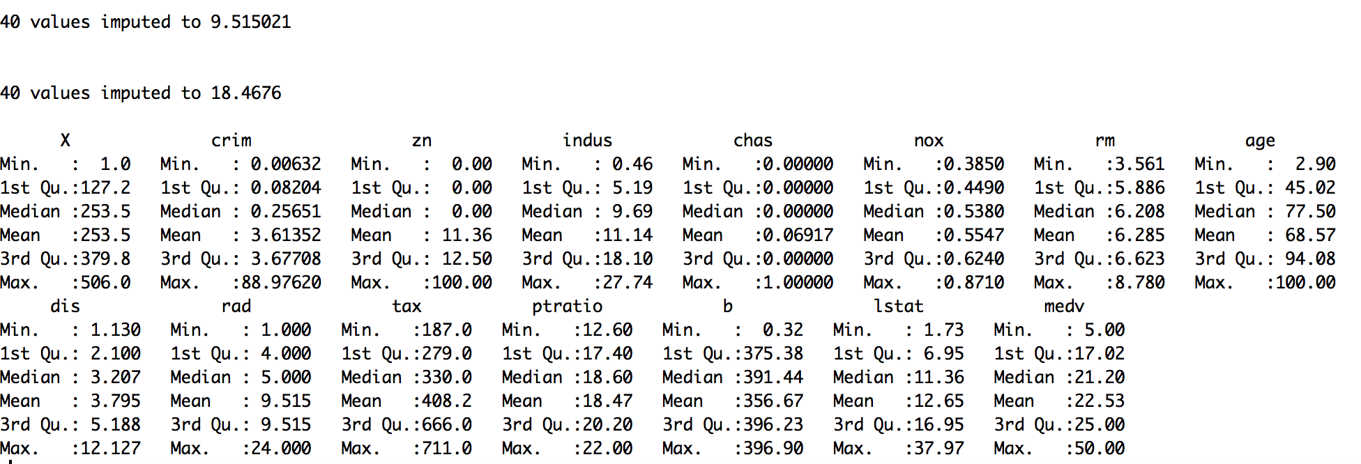
- Replace the missing values with mean, median, or mode:
#replace with mean
> housing.dat$ptratio <- impute(housing.dat$ptratio, mean)
> housing.dat$rad <- impute(housing.dat$rad, mean)

#replace with median
> housing.dat$ptratio <- impute(housing.dat$ptratio, median)
> housing.dat$rad <- impute(housing.dat$rad, median)

#replace with mode/constant value
> housing.dat$ptratio <- impute(housing.dat$ptratio, 18)
> housing.dat$rad <- impute(housing.dat$rad, 6)
Finally, verify the dataset with summary statistics:
> summary(housing.dat)
How it works...
When you have large numbers of observations in your dataset and all the classes to be predicted are sufficiently represented by the data points, then deleting missing observations would not introduce bias or disproportionality of output classes.
In the housing.dat dataset, we saw from the summary statistics that the dataset has two columns, ptratio and rad, with missing values.
The na.omit() function lets you remove all the missing values from all the columns of your dataset, whereas the complete.cases() function lets you remove the missing values from some particular column/columns.
Sometimes, particular variable/variables might have more missing values than the rest of the variables in the dataset. Then it is better to remove that variable unless it is a really important predictor that makes a lot of business sense. Assigning NULL to a variable is an easy way of removing it from the dataset.
In both, the given way of handling missing values through the deletion approach reduces the total number of observations (or rows) from the dataset. Instead of removing missing observations or removing a variable with many missing values, replacing the missing values with the mean, median, or mode is often a crude way of treating the missing values. Depending on the context, such as if the variation is low or if the variable has low leverage over the response/target, such a naive approximation is acceptable and could possibly give satisfactory results. The impute() function in the Hmisc library provides an easy way to replace the missing value with the mean, median, or mode (constant).
There's more...
Sometime it is better to understand the missing pattern in the dataset through visualization before taking further decision about elimination or imputation of the missing values.
Understanding missing data pattern
Let us use the md.pattern() function from the mice package to get a better understanding of the pattern of missing data.
> library(mice)
> md.pattern(housing.dat)
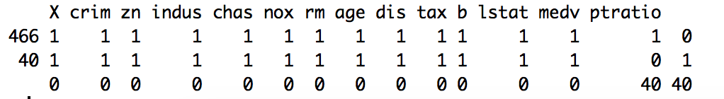
We can notice from the output above that 466 samples are complete, 40 samples miss only the ptratio value.
Next we will visualize the housing data to understand missing information using aggr_plot method from VIM package:
> library(VIM)
> aggr_plot <- aggr(housing.dat, col=c('blue','red'), numbers=TRUE, sortVars=TRUE, labels=names(housing.dat), cex.axis=.7, gap=3, ylab=c("Histogram of missing data","Pattern"))
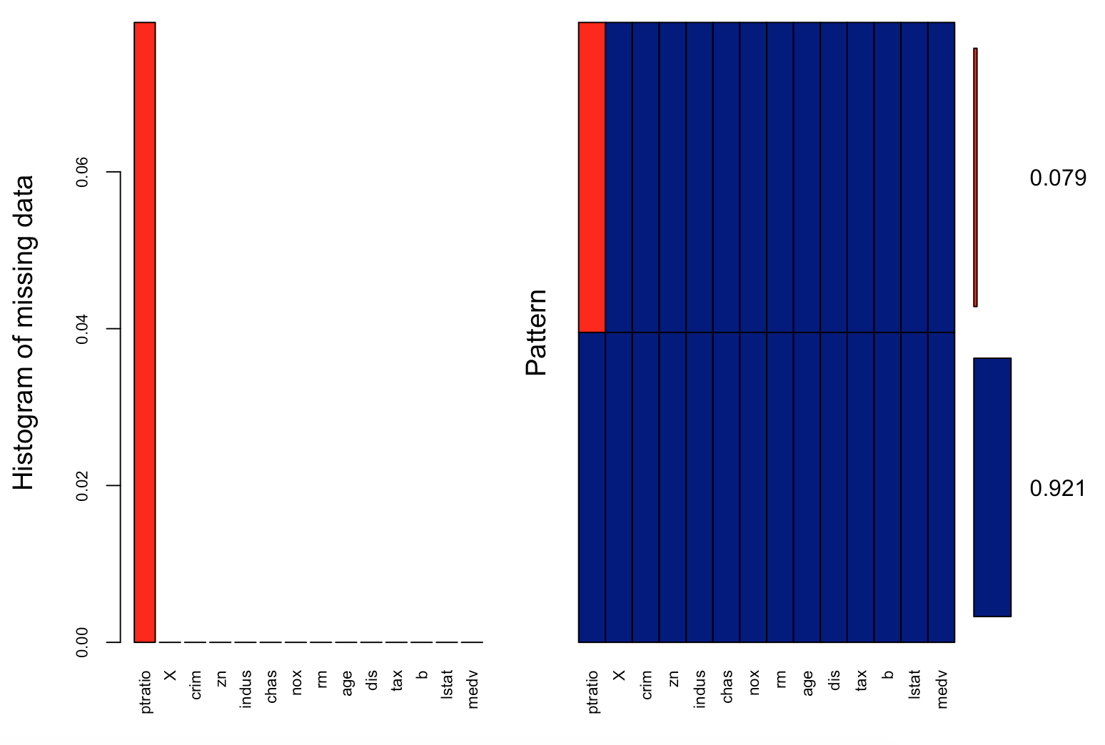
We can understand from the plot that almost 92.1% of the samples are complete and only 7.9% are missing information from the ptratio values.
Correcting data
In practice, raw data is rarely tidy, and is much harder to work with as a result. It is often said that 80 percent of data analysis is spent on the process of cleaning and correcting the data.
In this recipe, you will learn the best way to correctly layout your data to serve two major purposes:
- Making data suitable for software processing, whether that be mathematical functions, visualization, and others
- Revealing information and insights
Getting ready
Download the files for this chapter and store the USArrests.csv file in your R working directory. You should also install the tidyr package using the following command.
> install.packages("tidyr")
> library(tidyr)
> crimeData <- read.csv("USArrests.csv",stringsAsFactors = FALSE)
How to do it...
Follow these steps to correct the data from your dataset.
- View some records of the dataset:
> View(crimeData)
- Add the column name state in the dataset:
> crimeData <- cbind(state = rownames(crimeData), crimeData)
- Gather all the variables between Murder and UrbanPop:
> crimeData.1 <- gather(crimeData,
key = "crime_type",
value = "arrest_estimate",
Murder:UrbanPop)

 > crimeData.1
- Gather all the columns except the column state:
> crimeData.2 <- gather(crimeData,
key = "crime_type",
value = "arrest_estimate",
-state)

 > crimeData.2
- Gather only the Murder and Assault columns:
> crimeData.3 <- gather(crimeData,
key = "crime_type",
value = "arrest_estimate",
Murder, Assault)

 > crimeData.3
- Spread crimeData.2 to turn a pair of key:value (crime_typ:arrest_estimate) columns into a set of tidy columns
> crimeData.4 <- spread(crimeData.2,
key = "crime_type",
value = "arrest_estimate"
)
 > crimeData.4
How it works...
Correct data format is crucial for facilitating the tasks of data analysis, including data manipulation, modeling, and visualization. The tidy data arranges values so that the relationships in the data parallel the structure of the data frame. Every tidy dataset is based on two basic principles:
- Each variable is saved in its own column
- Each observation is saved in its own row
In the crimeData dataframe, the row names were states, hence we used the function cbind() to add a column named state in the dataframe. The function gather() collapses multiple columns into key-value pairs. It makes wide data longer. The gather() function basically takes four arguments, data (dataframe), key (column name representing new variable), value (column name representing variable values), and names of the columns to gather (or not gather).
In the crimeData.2 data, all column names (except state) were collapsed into a single key column crime_type and their values were put into a value column arrest_estimate.
And, in the crimeData.3 data, the two columns Murder and Assault were collapsed and the remaining columns (state, UrbanPop, and Rape) were
duplicated.
The function spread() does the reverse of gather(). It takes two columns (key and value) and spreads them into multiple columns. It makes long data wider. The spread() function takes three arguments in general, data (dataframe), key (column values to convert to multiple columns), and value (single column value to convert to multiple columns' values).
There's more...
Beside the spread() and gather() functions, there are two more important functions in the tidyr package that help to make data tidy.
Combining multiple columns to single columns
The unite() function takes multiple columns and pastes them together into one column:
> crimeData.5 <- unite(crimeData,
                  col = "Murder_Assault",
                  Murder, Assault,
                  sep = "_")
 > crimeData.5
We combine the columns Murder and Assault from the crimeData
data-frame to generate a new column Murder_Assault, having the values separated by _.
Splitting single column to multiple columns
The separate() function is the reverse of unite(). It takes values inside a single character column and separates them into multiple columns:
> crimeData.6 <- separate_(crimeData.5,
         col = "Murder_Assault",
         into = c("Murder", "Assault"),
         sep = "_")
>crimeData.6
Imputing data
Missing values are considered to be the first obstacle in data analysis and predictive modeling. In most statistical analysis methods, list-wise deletion is the default method used to impute missing values, as shown in the earlier recipe. However, these methods are not quite good enough, since deletion could lead to information loss and replacement with simple mean or median, which doesn't take into account the uncertainty in missing values.
Hence, this recipe will show you the multivariate imputation techniques to handle missing values using prediction.
Getting ready
Make sure that the housing-with-missing-value.csv file from the code files of this chapter is in your R working directory.
You should also install the mice package using the following command:
> install.packages("mice")
> library(mice)
> housingData <- read.csv("housing-with-missing-value.csv",header = TRUE, stringsAsFactors = FALSE)
How to do it...
Follow these steps to impute data:
- Perform multivariate imputation:
#imputing only two columns having missing values
> columns=c("ptratio","rad")

> imputed_Data <- mice(housingData[,names(housingData) %in% columns], m=5, maxit = 50, method = 'pmm', seed = 500)

>summary(imputed_Data)
- Generate complete data:
> completeData <- complete(imputed_Data)
- Replace the imputed column values with the housing.csv dataset:
> housingData$ptratio <- completeData$ptratio
> housingData$rad <- completeData$rad
- Check for missing values:
> anyNA(housingData)
How it works...
As we already know from our earlier recipe, the housing.csv dataset contains two columns, ptratio and rad, with missing values.
The mice library in R uses a predictive approach and assumes that the missing data is Missing at Random (MAR), and creates multivariate imputations via chained equations to take care of uncertainty in the missing values. It implements the imputation in just two steps: using mice() to build the model and complete() to generate the completed data.
The mice() function takes the following parameters:
- m: It refers to the number of imputed datasets it creates internally. Default is five.
- maxit: It refers to the number of iterations taken to impute the missing values.
- method: It refers to the method used in imputation. The default imputation method (when no argument is specified) depends on the measurement level of the target column and is specified by the defaultMethod argument, where defaultMethod = c("pmm", "logreg", "polyreg", "polr").
- logreg: Logistic regression (factor column, two levels).
- polyreg: Polytomous logistic regression (factor column, greater than or equal to two levels).
- polr: Proportional odds model (ordered column, greater than or equal to two levels).
We have used predictive mean matching (pmm) for this recipe to impute the missing values in the dataset.
The anyNA() function returns a Boolean value to indicate the presence or absence of missing values (NA) in the dataset.
There's more...
Previously, we used the impute() function from the Hmisc library to simply impute the missing value using defined statistical methods (mean, median, and mode). However, Hmisc also has the aregImpute() function that allows mean imputation using additive regression, bootstrapping, and predictive mean matching:
> impute_arg <- aregImpute(~ ptratio + rad , data = housingData, n.impute = 5)

> impute_arg
argImpute() automatically identifies the variable type and treats it accordingly, and the n.impute parameter indicates the number of multiple imputations, where five is recommended.
The output of impute_arg shows R² values for predicted missing values. The higher the value, the better the values predicted.
Check imputed variable values using the following command:
> impute_arg$imputed$rad
Detecting outliers
Outliers in data can distort predictions and affect the accuracy, if you don't detect and handle them appropriately, especially in the data preprocessing stage.
So, identifying the extreme values is important, as it can drastically introduce bias in the analytic pipeline and affect predictions. In this recipe, we will discuss the ways to detect outliers and how to handle them.
Getting ready
Download the files for this chapter and store the ozone.csv file in your R working directory. Read the file using the read.csv() command and save it in a variable:
> ozoneData <- read.csv("ozone.csv", stringsAsFactors=FALSE)
How to do it...
Perform the following steps to detect outliers in the dataset:
- Detect outliers in the univariate continuous variable:
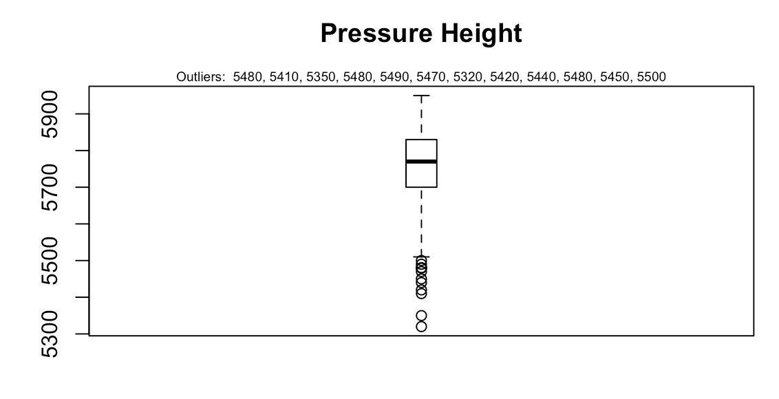
>outlier_values <- boxplot.stats(ozoneData$pressure_height)$out

>boxplot(ozoneData$pressure_height, main="Pressure Height", boxwex=0.1)

>mtext(paste("Outliers: ", paste(outlier_values, collapse=", ")), cex=0.6)
The output would be the following screenshot:
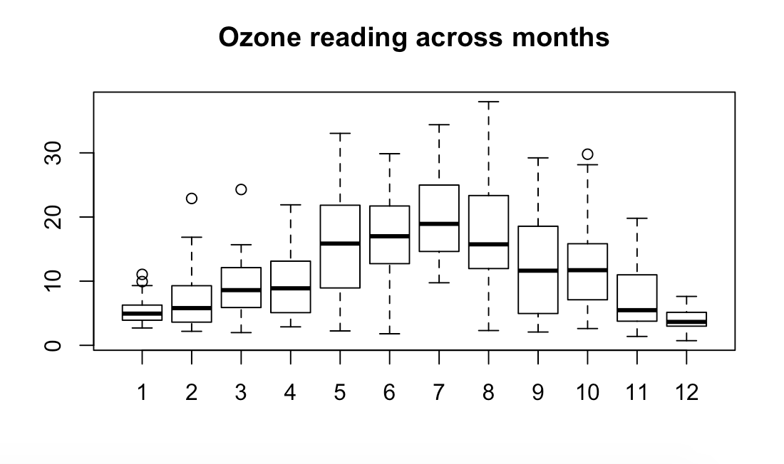
- Detect outliers in bivariate categorical variables:
> boxplot(ozone_reading ~ Month, data=ozoneData, main="Ozone reading across months")
The output would be the following screenshot:
How it works...
The most commonly used method to detect outliers is visualization of the data, through boxplot, histogram, or scatterplot.
The boxplot.stats()$out function fetches the values of data points that lie beyond the extremes of the whiskers. The boxwex attribute is a scale factor that is applied to all the boxes; it improves the appearance of the plot by making the boxes narrower. The mtext() function places a text outside the plot area, but within the plot window.
In the case of continuous variables, outliers are those observations that lie outside 1.5 * IQR, where Inter Quartile Range or IQR, is the difference between the 75th and 25th quartiles. The outliers in continuous variables show up as dots outside the whiskers of the boxplot.
In case of bivariate categorical variables, a clear pattern is noticeable and the change in the level of boxes suggests that Month seems to have an impact in ozone_reading. The outliers in respective categorical levels show up as dots outside the whiskers of the boxplot.
There's more...
Detecting and handling outliers depends mostly on your application. Once you have identified the outliers and you have decided to make amends as per the nature of the problem, you may consider one of the following approaches.
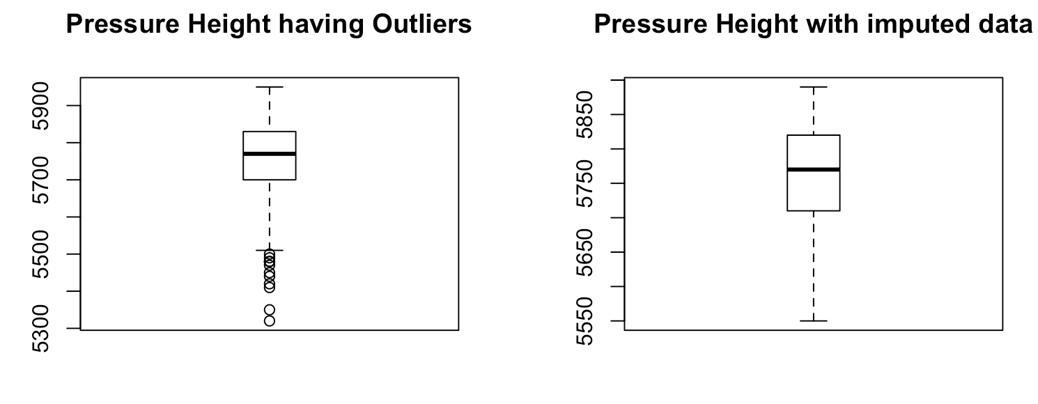
Treating the outliers with mean/median imputation
We can handle outliers with mean or median imputation by replacing the observations lower than the 5th percentile with mean and those higher than 95th percentile with median. We can use the same statistics, mean or median, to impute outliers in both directions:
> impute_outliers <- function(x,removeNA = TRUE){
    quantiles <- quantile( x, c(.05, .95 ),na.rm = removeNA )
    x[ x < quantiles[1] ] <- mean(x,na.rm = removeNA )
    x[ x > quantiles[2] ] <- median(x,na.rm = removeNA )
    x
}

> imputed_data <- impute_outliers(ozoneData$pressure_height)
Validate the imputed data through visualization:
> par(mfrow = c(1, 2))

> boxplot(ozoneData$pressure_height, main="Pressure Height having Outliers", boxwex=0.3)

> boxplot(imputed_data, main="Pressure Height with imputed data", boxwex=0.3)
The output would be the following screenshot:
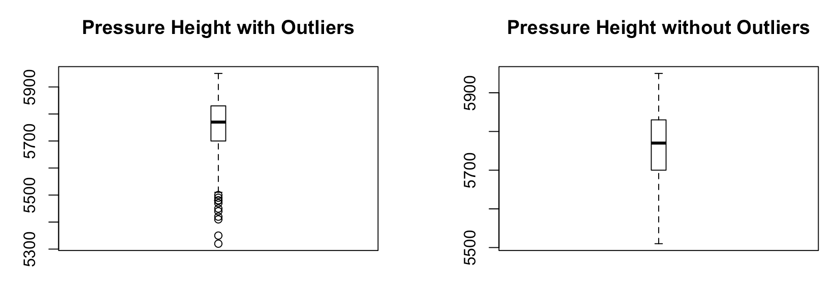
Handling extreme values with capping
To handle extreme values that lie outside the 1.5 * IQR(Inter Quartile Range) limits, we could cap them by replacing those observations that lie below the lower limit, with the value of 5th percentile and those that lie above the upper limit, with the value of 95th percentile, as shown in the following code:
> replace_outliers <- function(x, removeNA = TRUE) {
     pressure_height <- x
     qnt <- quantile(pressure_height, probs=c(.25, .75), na.rm = removeNA)
     caps <- quantile(pressure_height, probs=c(.05, .95), na.rm = removeNA)
     H <- 1.5 * IQR(pressure_height, na.rm = removeNA)
     pressure_height[pressure_height < (qnt[1] - H)] <- caps[1]
     pressure_height[pressure_height > (qnt[2] + H)] <- caps[2]
     pressure_height
 }

> capped_pressure_height <- replace_outliers(ozoneData$pressure_height)
Validate the capped variable capped_pressure_height through visualization:
> par(mfrow = c(1, 2))

> boxplot(ozoneData$pressure_height, main="Pressure Height with Outliers", boxwex=0.1)

> boxplot(capped_pressure_height, main="Pressure Height without Outliers", boxwex=0.1)
The output would be the following screenshot:
Transforming and binning values
Sometimes, transforming variables can also eliminate outliers. The natural log or square root of a value reduces the variation caused by extreme values. Some predictive analytics algorithms, such as decision trees, inherently deal with outliers by using binning techniques (a form of variable transformation).
Outlier detection with LOF
Local Outlier Factor or LOF is an algorithm implemented in DMwR package for identifying density-based local outliers, by comparing the local density of a point with that of its neighbors.
Now we will calculates the local outlier factors using the LOF algorithm using k number of neighbors:
> install.packages("DMwR")
> library(DMwR)
> outlier.scores <- lofactor(ozoneData, k=3)
Finally we will output the top 5 outlier by sorting the outlier score calculated above:
> outliers <- order(outlier.scores, decreasing=T)[1:5]
> print(outliers)