In this chapter, we will cover the following recipes:

• Array creation in Python
• Data preprocessing using mean removal
• Data scaling
• Normalization
• Binarization
• One-hot encoding
• Label encoding
• Building a linear regressor
• Computing regression accuracy
• Achieving model persistence
• Building a ridge regressor
• Building a polynomial regressor
• Estimating housing prices
• Computing the relative importance of features
• Estimating bicycle demand distribution

We will use various Python packages, such as NumPy, SciPy, scikit-learn, and Matplotlib, during the course of this book to build various things. If you use Windows, it is recommended that you use a SciPy-stack-compatible version of Python. You can check the list of compatible versions at http://www.scipy.org/install.html. These distributions come with all the necessary packages already installed. If you use MacOS X or Ubuntu, installing these packages is fairly straightforward. Here are some useful links for installation and documentation:

• NumPy: https://www.numpy.org/devdocs/user/install.html.
• SciPy: http://www.scipy.org/install.html.
• Scikit-learn: https://scikit-learn.org/stable/install.html.
• Matplotlib: https://matplotlib.org/users/installing.html.

Make sure that you have these packages installed on your machine before you proceed. In each recipe, we will give a detailed explanation of the functions that we will use in order to make it simple and fast.

Machine learning is a multidisciplinary field created at the intersection of, and with synergy between, computer science, statistics, neurobiology, and control theory. It has played a key role in various fields and has radically changed the vision of programming software. For humans, and more generally, for every living being, learning is a form of adaptation of a system to its environment through experience. This adaptation process must lead to improvement without human intervention. To achieve this goal, the system must be able to learn, which means that it must be able to extract useful information on a given problem by examining a series of examples associated with it.

If you are familiar with the basics of machine learning, you will certainly know what supervised learning is all about. To give you a quick refresher, supervised learning refers to building a machine learning model that is based on labeled samples. The algorithm generates a function which connects input values to a desired output via of a set of labeled examples, where each data input has its relative output data. This is used to construct predictive models. For example, if we build a system to estimate the price of a house based on various parameters, such as size, locality, and so on, we first need to create a database and label it. We need to tell our algorithm what parameters correspond to what prices. Based on this data, our algorithm will learn how to calculate the price of a house using the input parameters.

Unsupervised learning is in stark contrast to what we just discussed. There is no labeled data available here. The algorithm tries to acquire knowledge from general input without the help of a set of pre-classified examples that are used to build descriptive models. Let's assume that we have a bunch of data points, and we just want to separate them into multiple groups. We don't exactly know what the criteria of separation would be. So, an unsupervised learning algorithm will try to separate the given dataset into a fixed number of groups in the best possible way. We will discuss unsupervised learning in the upcoming chapters.

In the following recipes, we will look at various data preprocessing techniques.

Arrays are the essential elements of many programming languages. Arrays are sequential objects that behave very similarly to lists, except that the types of elements contained in them are constrained. The type is specified when the object is created using a single character called type code.

In this recipe, we will cover an array creation procedure. We will first create an array using the NumPy library, and then display its structure.

Let's see how to create an array in Python:

1. To start off, import the NumPy library as follows:

>> import numpy as np

We just imported a necessary package, numpy. This is the fundamental package for scientific computing with Python. It contains, among other things, the following:

• A powerful N-dimensional array object
• Sophisticated broadcasting functions
• Tools for integrating C, C++, and FORTRAN code
• Useful linear algebra, Fourier transform, and random number capabilities

Besides its obvious uses, NumPy is also used as an efficient multidimensional container of generic data. Arbitrary data types can be found. This enables NumPy to integrate with different types of databases.

2. Let's create some sample data. Add the following line to the Python Terminal:

>> data = np.array([[3, -1.5, 2, -5.4], [0, 4, -0.3, 2.1], [1, 3.3, -1.9, -4.3]])

The np.array function creates a NumPy array. A NumPy array is a grid of values, all of the same type, indexed by a tuple of non-negative integers. rank and shape are essential features of a NumPy array. The rank variable is the number of dimensions of the array. The shape variable is a tuple of integers that returns the size of the array along each dimension.

3. We display the newly created array with this snippet:

>> print(data)

The following result is returned:

[[ 3. -1.5  2.  -5.4]
 [ 0.  4.  -0.3  2.1]
 [ 1.  3.3 -1.9 -4.3]]

We are now ready to operate on this data.

NumPy is an extension package in the Python environment that is fundamental for scientific calculation. This is because it adds to the tools that are already available, the typical features of N-dimensional arrays, element-by-element operations, a massive number of mathematical operations in linear algebra, and the ability to integrate and recall source code written in C, C++, and FORTRAN. In this recipe, we learned how to create an array using the NumPy library.

NumPy provides us with various tools for creating an array. For example, to create a one-dimensional array of equidistant values with numbers from 0 to 10, we would use the arange() function, as follows:

>> NpArray1 = np.arange(10)
>> print(NpArray1)

The following result is returned:

[0 1 2 3 4 5 6 7 8 9]

To create a numeric array from 0 to 50, with a step of 5 (using a predetermined step between successive values), we will write the following code:

>> NpArray2 = np.arange(10, 100, 5)
>> print(NpArray2)

The following array is printed:

[10 15 20 25 30 35 40 45 50 55 60 65 70 75 80 85 90 95]

Also, to create a one-dimensional array of 50 numbers between two limit values and that are equidistant in this range, we will use the linspace() function:

>> NpArray3 = np.linspace(0, 10, 50)
>> print(NpArray3)

The following result is returned:

[ 0. 0.20408163 0.40816327 0.6122449 0.81632653 1.02040816
 1.2244898 1.42857143 1.63265306 1.83673469 2.04081633 2.24489796
 2.44897959 2.65306122 2.85714286 3.06122449 3.26530612 3.46938776
 3.67346939 3.87755102 4.08163265 4.28571429 4.48979592 4.69387755
 4.89795918 5.10204082 5.30612245 5.51020408 5.71428571 5.91836735
 6.12244898 6.32653061 6.53061224 6.73469388 6.93877551 7.14285714
 7.34693878 7.55102041 7.75510204 7.95918367 8.16326531 8.36734694
 8.57142857 8.7755102 8.97959184 9.18367347 9.3877551 9.59183673
 9.79591837 10. ]

These are just some simple samples of NumPy. In the following sections, we will delve deeper into the topic.

• NumPy developer guide (https://docs.scipy.org/doc/numpy/dev/).
• NumPy tutorial (https://docs.scipy.org/doc/numpy/user/quickstart.html).
• NumPy reference (https://devdocs.io/numpy~1.12/).

In the real world, we usually have to deal with a lot of raw data. This raw data is not readily ingestible by machine learning algorithms. To prepare data for machine learning, we have to preprocess it before we feed it into various algorithms. This is an intensive process that takes plenty of time, almost 80 percent of the entire data analysis process, in some scenarios. However, it is vital for the rest of the data analysis workflow, so it is necessary to learn the best practices of these techniques. Before sending our data to any machine learning algorithm, we need to cross check the quality and accuracy of the data. If we are unable to reach the data stored in Python correctly, or if we can't switch from raw data to something that can be analyzed, we cannot go ahead. Data can be preprocessed in many ways—standardization, scaling, normalization, binarization, and one-hot encoding are some examples of preprocessing techniques. We will address them through simple examples.

Standardization or mean removal is a technique that simply centers data by removing the average value of each characteristic, and then scales it by dividing non-constant characteristics by their standard deviation. It's usually beneficial to remove the mean from each feature so that it's centered on zero. This helps us remove bias from features. The formula used to achieve this is the following:

Standardization results in the rescaling of features, which in turn represents the properties of a standard normal distribution:

• mean = 0
• sd = 1

In this formula, mean is the mean and sd is the standard deviation from the mean.

Let's see how to preprocess data in Python:

1. Let's start by importing the library:

>> from sklearn import preprocessing

The sklearn library is a free software machine learning library for the Python programming language. It features various classification, regression, and clustering algorithms, including support vector machines (SVMs), random forests, gradient boosting, k-means, and DBSCAN, and is designed to interoperate with the Python numerical and scientific libraries, NumPy and SciPy.

2. To understand the outcome of mean removal on our data, we first visualize the mean and standard deviation of the vector we have just created:

>> print("Mean: ",data.mean(axis=0))
>> print("Standard Deviation: ",data.std(axis=0))

The mean() function returns the sample arithmetic mean of data, which can be a sequence or an iterator. The std() function returns the standard deviation, a measure of the distribution of the array elements. The axis parameter specifies the axis along which these functions are computed (0 for columns, and 1 for rows).

The following results are returned:

Mean: [ 1.33333333 1.93333333 -0.06666667 -2.53333333]
Standard Deviation: [1.24721913 2.44449495 1.60069429 3.30689515]

3. Now we can proceed with standardization:

>> data_standardized = preprocessing.scale(data)

The preprocessing.scale() function standardizes a dataset along any axis. This method centers the data on the mean and resizes the components in order to have a unit variance.

4. Now we recalculate the mean and standard deviation on the standardized data:

>> print("Mean standardized data: ",data_standardized.mean(axis=0))
>> print("Standard Deviation standardized data: ",data_standardized.std(axis=0))

The following results are returned:

Mean standardized data: [ 5.55111512e-17 -1.11022302e-16 -7.40148683e-17 -7.40148683e-17]
Standard Deviation standardized data: [1. 1. 1. 1.]

You can see that the mean is almost 0 and the standard deviation is 1.

The sklearn.preprocessing package provides several common utility functions and transformer classes to modify the features available in a representation that best suits our needs. In this recipe, the scale() function has been used (z-score standardization). In summary, the z-score (also called the standard score) represents the number of standard deviations by which the value of an observation point or data is greater than the mean value of what is observed or measured. Values more than the mean have positive z-scores, while values less than the mean have negative z-scores. The z-score is a quantity without dimensions that is obtained by subtracting the population's mean from a single rough score and then dividing the difference by the standard deviation of the population.

Standardization is particularly useful when we do not know the minimum and maximum for data distribution. In this case, it is not possible to use other forms of data transformation. As a result of the transformation, the normalized values do not have a minimum and a fixed maximum. Moreover, this technique is not influenced by the presence of outliers, or at least not the same as other methods.

• Scikit-learn's official documentation of the sklearn.preprocessing.scale() function: https://scikit-learn.org/stable/modules/generated/sklearn.preprocessing.scale.html.

The values of each feature in a dataset can vary between random values. So, sometimes it is important to scale them so that this becomes a level playing field. Through this statistical procedure, it's possible to compare identical variables belonging to different distributions and different variables.

We'll use the min-max method (usually called feature scaling) to get all of the scaled data in the range [0, 1]. The formula used to achieve this is as follows:

To scale features between a given minimum and maximum value—in our case, between 0 and 1—so that the maximum absolute value of each feature is scaled to unit size, the preprocessing.MinMaxScaler() function can be used.

Let's see how to scale data in Python:

1. Let's start by defining the data_scaler variable:

>> data_scaler = preprocessing.MinMaxScaler(feature_range=(0, 1))

2. Now we will use the fit_transform() method, which fits the data and then transforms it (we will use the same data as in the previous recipe):

>> data_scaled = data_scaler.fit_transform(data)

A NumPy array of a specific shape is returned. To understand how this function has transformed data, we display the minimum and maximum of each column in the array.

3. First, for the starting data and then for the processed data:

>> print("Min: ",data.min(axis=0))
>> print("Max: ",data.max(axis=0))

The following results are returned:

Min: [ 0. -1.5 -1.9 -5.4]
Max: [3. 4. 2. 2.1]

4. Now, let's do the same for the scaled data using the following code:

>> print("Min: ",data_scaled.min(axis=0))
>> print("Max: ",data_scaled.max(axis=0))

The following results are returned:

Min: [0. 0. 0. 0.]
Max: [1. 1. 1. 1.]

After scaling, all the feature values range between the specified values.

5. To display the scaled array, we will use the following code:

>> print(data_scaled)

The output will be displayed as follows:

[[ 1.          0.          1.          0.        ] 
 [ 0.          1.          0.41025641  1.        ]
 [ 0.33333333  0.87272727  0.          0.14666667]]

Now, all the data is included in the same interval.

When data has different ranges, the impact on response variables might be higher than the one with a lesser numeric range, which can affect the prediction accuracy. Our goal is to improve predictive accuracy and ensure this doesn't happen. Hence, we may need to scale values under different features so that they fall within a similar range. Through this statistical procedure, it's possible to compare identical variables belonging to different distributions and different variables or variables expressed in different units.

Feature scaling consists of limiting the excursion of a set of values within a certain predefined interval. It guarantees that all functionalities have the exact same scale, but does not handle anomalous values well. This is because extreme values become the extremes of the new range of variation. In this way, the actual values are compressed by keeping the distance to the anomalous values.

• Scikit-learn's official documentation of the sklearn.preprocessing.MinMaxScaler() function: https://scikit-learn.org/stable/modules/generated/sklearn.preprocessing.MinMaxScaler.html.

Data normalization is used when you want to adjust the values in the feature vector so that they can be measured on a common scale. One of the most common forms of normalization that is used in machine learning adjusts the values of a feature vector so that they sum up to 1.

To normalize data, the preprocessing.normalize() function can be used. This function scales input vectors individually to a unit norm (vector length). Three types of norms are provided, l₁, l₂, or max, and they are explained next. If x is the vector of covariates of length n, the normalized vector is y=x/z, where z is defined as follows:

The norm is a function that assigns a positive length to each vector belonging to a vector space, except 0.

Let's see how to normalize data in Python:

1. As we said, to normalize data, the preprocessing.normalize() function can be used as follows (we will use the same data as in the previous recipe):

>> data_normalized = preprocessing.normalize(data, norm='l1', axis=0)

2. To display the normalized array, we will use the following code:

>> print(data_normalized)

The following output is returned:

[[ 0.75 -0.17045455  0.47619048  -0.45762712]
 [ 0.    0.45454545 -0.07142857   0.1779661 ]
 [ 0.25  0.375      -0.45238095  -0.36440678]]

This is used a lot to make sure that datasets don't get boosted artificially due to the fundamental nature of their features.

3. As already mentioned, the normalized array along the columns (features) must return a sum equal to 1. Let's check this for each column:

>> data_norm_abs = np.abs(data_normalized)
>> print(data_norm_abs.sum(axis=0))

In the first line of code, we used the np.abs() function to evaluate the absolute value of each element in the array. In the second row of code, we used the sum() function to calculate the sum of each column (axis=0). The following results are returned:

[1. 1. 1. 1.]

Therefore, the sum of the absolute value of the elements of each column is equal to 1, so the data is normalized.

In this recipe, we normalized the data at our disposal to the unitary norm. Each sample with at least one non-zero component was rescaled independently of other samples so that its norm was equal to one.

Scaling inputs to a unit norm is a very common task in text classification and clustering problems.

• Scikit-learn's official documentation of the sklearn.preprocessing.normalize() function: https://scikit-learn.org/stable/modules/generated/sklearn.preprocessing.normalize.html.

Binarization is used when you want to convert a numerical feature vector into a Boolean vector. In the field of digital image processing, image binarization is the process by which a color or grayscale image is transformed into a binary image, that is, an image with only two colors (typically, black and white).

This technique is used for the recognition of objects, shapes, and, specifically, characters. Through binarization, it is possible to distinguish the object of interest from the background on which it is found. Skeletonization is instead an essential and schematic representation of the object, which generally preludes the subsequent real recognition.

Let's see how to binarize data in Python:

1. To binarize data, we will use the preprocessing.Binarizer() function as follows (we will use the same data as in the previous recipe):

>> data_binarized = preprocessing.Binarizer(threshold=1.4).transform(data)

The preprocessing.Binarizer() function binarizes data according to an imposed threshold. Values greater than the threshold map to 1, while values less than or equal to the threshold map to 0. With the default threshold of 0, only positive values map to 1. In our case, the threshold imposed is 1.4, so values greater than 1.4 are mapped to 1, while values less than 1.4 are mapped to 0.

2. To display the binarized array, we will use the following code:

>> print(data_binarized)

The following output is returned:

[[ 1.  0.  1.  0.]
 [ 0.  1.  0.  1.]
 [ 0.  1.  0.  0.]]

This is a very useful technique that's usually used when we have some prior knowledge of the data.

In this recipe, we binarized the data. The fundamental idea of ​​this technique is to draw a fixed demarcation line. It is therefore a matter of finding an appropriate threshold and affirming that all the points of the image whose light intensity is below a certain value belong to the object (background), and all the points with greater intensity belong to the background (object).

Binarization is a widespread operation on count data, in which the analyst can decide to consider only the presence or absence of a characteristic rather than a quantified number of occurrences. Otherwise, it can be used as a preprocessing step for estimators that consider random Boolean variables.

• Scikit-learn's official documentation of the sklearn.preprocessing.Binarizer() function: https://scikit-learn.org/stable/modules/generated/sklearn.preprocessing.Binarizer.html.

We often deal with numerical values that are sparse and scattered all over the place. We don't really need to store these values. This is where one-hot encoding comes into the picture. We can think of one-hot encoding as a tool that tightens feature vectors. It looks at each feature and identifies the total number of distinct values. It uses a one-of-k scheme to encode values. Each feature in the feature vector is encoded based on this scheme. This helps us to be more efficient in terms of space.

Let's say we are dealing with four-dimensional feature vectors. To encode the nth feature in a feature vector, the encoder will go through the nth feature in each feature vector and count the number of distinct values. If the number of distinct values is k, it will transform the feature into a k-dimensional vector where only one value is 1 and all other values are 0. Let's take a simple example to understand how this works.

Let's see how to encode data in Python:

1. Let's take an array with four rows (vectors) and three columns (features):

>> data = np.array([[1, 1, 2], [0, 2, 3], [1, 0, 1], [0, 1, 0]])
>> print(data)

The following result is printed:

[[1 1 2]
 [0 2 3]
 [1 0 1]
 [0 1 0]]

Let's analyze the values present in each column (feature):

• The first feature has two possible values: 0, 1
• The second feature has three possible values: 0, 1, 2
• The third feature has four possible values: 0, 1, 2, 3

So, overall, the sum of the possible values present in each feature is given by 2 + 3 + 4 = 9. This means that 9 entries are required to uniquely represent any vector. The three features will be represented as follows:

• Feature 1 starts at index 0
• Feature 2 starts at index 2
• Feature 3 starts at index 5

2. To encode categorical integer features as a one-hot numeric array, the preprocessing.OneHotEncoder() function can be used as follows:

>> encoder = preprocessing.OneHotEncoder()
>> encoder.fit(data)

The first row of code sets the encoder, then the fit() function fits the OneHotEncoder object to a data array.

3. Now we can transform the data array using one-hot encoding. To do this, the transform() function will be used as follows:

>> encoded_vector = encoder.transform([[1, 2, 3]]).toarray()

If you were to print encoded_vector, the expected output would be:

[[0. 1. 0. 0. 1. 0. 0. 0. 1.]]

The result is clear: the first feature (1) has an index of 1, the second feature (3) has an index of 4, and the third feature (3) has an index of 8. As we can verify, only these positions are occupied by a 1; all the other positions have a 0. Remember that Python indexes the positions starting from 0, so the 9 entries will have indexes from 0 to 8.

The preprocessing.OneHotEncoder() function encodes categorical integer features as a one-hot numeric array. Starting from an array of integers or strings that denotes the values assumed by categorical characteristics (discrete), this function encodes the characteristics using a one-hot coding scheme, returning dummy variables. This creates a binary column for each category and returns a sparse array or a dense array.

It often happens that you have to convert categorical data. This is due to the fact that many machine learning algorithms can't work directly with categorical data. To use these methods, it is necessary to first transform categorical data into numerical data. This is required for both input and output variables.

• Scikit-learn's official documentation of the sklearn.preprocessing.OneHotEncoder() function: https://scikit-learn.org/stable/modules/generated/sklearn.preprocessing.OneHotEncoder.html.

In supervised learning, we usually deal with a variety of labels. These can be either numbers or words. If they are numbers, then the algorithm can use them directly. However, labels often need to be in a human-readable form. So, people usually label the training data with words.

Label encoding refers to transforming word labels into a numerical form so that algorithms can understand how to operate on them. Let's take a look at how to do this.

Let's see how to carry out label encoding in Python:

1. Create a new Python file and import the preprocessing() package:

>> from sklearn import preprocessing

2. This package contains various functions that are needed for data preprocessing. To encode labels with a value between 0 and n_classes-1, the preprocessing.LabelEncoder() function can be used. Let's define the label encoder, as follows:

>> label_encoder = preprocessing.LabelEncoder()

3. The label_encoder object knows how to understand word labels. Let's create some labels:

>> input_classes = ['audi', 'ford', 'audi', 'toyota', 'ford', 'bmw']

4. We are now ready to encode these labels—first, the fit() function is used to fit the label encoder, and then the class mapping encoders are printed:

>> label_encoder.fit(input_classes)
>> print("Class mapping: ")
>> for i, item in enumerate(label_encoder.classes_):
...    print(item, "-->", i)

5. Run the code, and you will see the following output on your Terminal:

Class mapping:
audi --> 0
bmw --> 1
ford --> 2
toyota --> 3

6. As shown in the preceding output, the words have been transformed into zero-indexed numbers. Now, when you encounter a set of labels, you can simply transform them, as follows:

>> labels = ['toyota', 'ford', 'audi']
>> encoded_labels = label_encoder.transform(labels)
>> print("Labels =", labels)
>> print("Encoded labels =", list(encoded_labels))

Here is the output that you'll see on your Terminal:

Labels = ['toyota', 'ford', 'audi']
Encoded labels = [3, 2, 0]

7. This is way easier than manually maintaining mapping between words and numbers. You can check the correctness by transforming numbers back into word labels:

>> encoded_labels = [2, 1, 0, 3, 1]
>> decoded_labels = label_encoder.inverse_transform(encoded_labels)
>> print("Encoded labels =", encoded_labels)
>> print("Decoded labels =", list(decoded_labels))

To transform labels back to their original encoding, the inverse_transform() function has been applied. Here is the output:

Encoded labels = [2, 1, 0, 3, 1]
Decoded labels = ['ford', 'bmw', 'audi', 'toyota', 'bmw']

As you can see, the mapping is preserved perfectly.

In this recipe, we used the preprocessing.LabelEncoder() function to transform word labels into numerical form. To do this, we first set up a series of labels to as many car brands. We then turned these labels into numerical values. Finally, to verify the operation of the procedure, we printed the values corresponding to each class labeled.

In the last two recipes, Label encoding and One-hot encoding, we have seen how to transform data. Both methods are suitable for dealing with categorical data. But what are the pros and cons of the two methodologies? Let's take a look:

• Label encoding can transform categorical data into numeric data, but the imposed ordinality creates problems if the obtained values are submitted to mathematical operations.
• One-hot encoding has the advantage that the result is binary rather than ordinal, and that everything is in an orthogonal vector space. The disadvantage is that for high cardinality, the feature space can explode.

• Scikit-learn's official documentation on the sklearn.preprocessing.LabelEncoder() function: https://scikit-learn.org/stable/modules/generated/sklearn.preprocessing.LabelEncoder.html.

Linear regression refers to finding the underlying function with the help of linear combination of input variables. The previous example had an input variable and an output variable. A simple linear regression is easy to understand, but represents the basis of regression techniques. Once these concepts are understood, it will be easier for us to address the other types of regression.

Consider the following diagram:

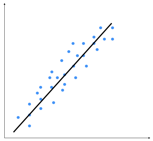
The linear regression method consists of precisely identifying a line that is capable of representing point distribution in a two-dimensional plane, that is, if the points corresponding to the observations are near the line, then the chosen model will be able to describe the link between the variables effectively.

In theory, there are an infinite number of lines that may approximate the observations, while in practice, there is only one mathematical model that optimizes the representation of the data. In the case of a linear mathematical relationship, the observations of the y variable can be obtained by a linear function of the observations of the x variable. For each observation, we will use the following formula:

In the preceding formula, x is the explanatory variable and y is the response variable. The α and β parameters, which represent the slope of the line and the intercept with the y-axis respectively, must be estimated based on the observations collected for the two variables included in the model.

The slope, α, is of particular interest, that is, the variation of the mean response for every single increment of the explanatory variable. What about a change in this coefficient? If the slope is positive, the regression line increases from left to right, and if the slope is negative, the line decreases from left to right. When the slope is zero, the explanatory variable has no effect on the value of the response. But it is not just the sign of α that establishes the weight of the relationship between the variables. More generally, its value is also important. In the case of a positive slope, the mean response is higher when the explanatory variable is higher, while in the case of a negative slope, the mean response is lower when the explanatory variable is higher.

The main aim of linear regression is to get the underlying linear model that connects the input variable to the output variable. This in turn reduces the sum of squares of differences between the actual output and the predicted output using a linear function. This method is called ordinary least squares. In this method, the coefficients are estimated by determining numerical values that minimize the sum of the squared deviations between the observed responses and the fitted responses, according to the following equation:

This quantity represents the sum of the squares of the distances to each experimental datum (x_i, y_i) from the corresponding point on the straight line.

You might say that there might be a curvy line out there that fits these points better, but linear regression doesn't allow this. The main advantage of linear regression is that it's not complex. If you go into non-linear regression, you may get more accurate models, but they will be slower. As shown in the preceding diagram, the model tries to approximate the input data points using a straight line. Let's see how to build a linear regression model in Python.

Regression is used to find out the relationship between input data and the continuously-valued output data. This is generally represented as real numbers, and our aim is to estimate the core function that calculates the mapping from the input to the output. Let's start with a very simple example. Consider the following mapping between input and output:

1 --> 2
3 --> 6
4.3 --> 8.6
7.1 --> 14.2

If I ask you to estimate the relationship between the inputs and the outputs, you can easily do this by analyzing the pattern. We can see that the output is twice the input value in each case, so the transformation would be as follows:

This is a simple function, relating the input values with the output values. However, in the real world, this is usually not the case. Functions in the real world are not so straightforward!

You have been provided with a data file called VehiclesItaly.txt. This contains comma-separated lines, where the first element is the input value and the second element is the output value that corresponds to this input value. Our goal is to find the linear regression relation between the vehicle registrations in a state and the population of a state. You should use this as the input argument. As anticipated, the Registrations variable contains the number of vehicles registered in Italy and the Population variable contains the population of the different regions.

Let's see how to build a linear regressor in Python:

1. Create a file called regressor.py and add the following lines:

filename = "VehiclesItaly.txt"
X = []
y = []
with open(filename, 'r') as f:
    for line in f.readlines():
        xt, yt = [float(i) for i in line.split(',')]
        X.append(xt)
        y.append(yt)

We just loaded the input data into X and y, where X refers to the independent variable (explanatory variables) and y refers to the dependent variable (response variable). Inside the loop in the preceding code, we parse each line and split it based on the comma operator. We then convert them into floating point values and save them in X and y.

2. When we build a machine learning model, we need a way to validate our model and check whether it is performing at a satisfactory level. To do this, we need to separate our data into two groups—a training dataset and a testing dataset. The training dataset will be used to build the model, and the testing dataset will be used to see how this trained model performs on unknown data. So, let's go ahead and split this data into training and testing datasets:

num_training = int(0.8 * len(X))
num_test = len(X) - num_training

import numpy as np

# Training data
X_train = np.array(X[:num_training]).reshape((num_training,1))
y_train = np.array(y[:num_training])

# Test data
X_test = np.array(X[num_training:]).reshape((num_test,1))
y_test = np.array(y[num_training:])

First, we have put aside 80% of the data for the training dataset and the remaining 20% is for the testing dataset. Then, we have built four arrays: X_train, X_test,y_train, and y_test.

3. We are now ready to train the model. Let's create a regressor object, as follows:

from sklearn import linear_model

# Create linear regression object
linear_regressor = linear_model.LinearRegression()

# Train the model using the training sets
linear_regressor.fit(X_train, y_train)

First, we have imported linear_model methods from the sklearn library, which are methods used for regression, wherein the target value is expected to be a linear combination of the input variables. Then, we have used the LinearRegression() function, which performs ordinary least squares linear regression. Finally, the fit() function is used to fit the linear model. Two parameters are passed—training data (X_train), and target values (y_train).

4. We just trained the linear regressor, based on our training data. The fit() method takes the input data and trains the model. To see how it all fits, we have to predict the training data with the model fitted:

y_train_pred = linear_regressor.predict(X_train)

5. To plot the outputs, we will use the matplotlib library as follows:

import matplotlib.pyplot as plt
plt.figure()
plt.scatter(X_train, y_train, color='green')
plt.plot(X_train, y_train_pred, color='black', linewidth=4)
plt.title('Training data')
plt.show()

When you run this in the Terminal, the following diagram is shown:

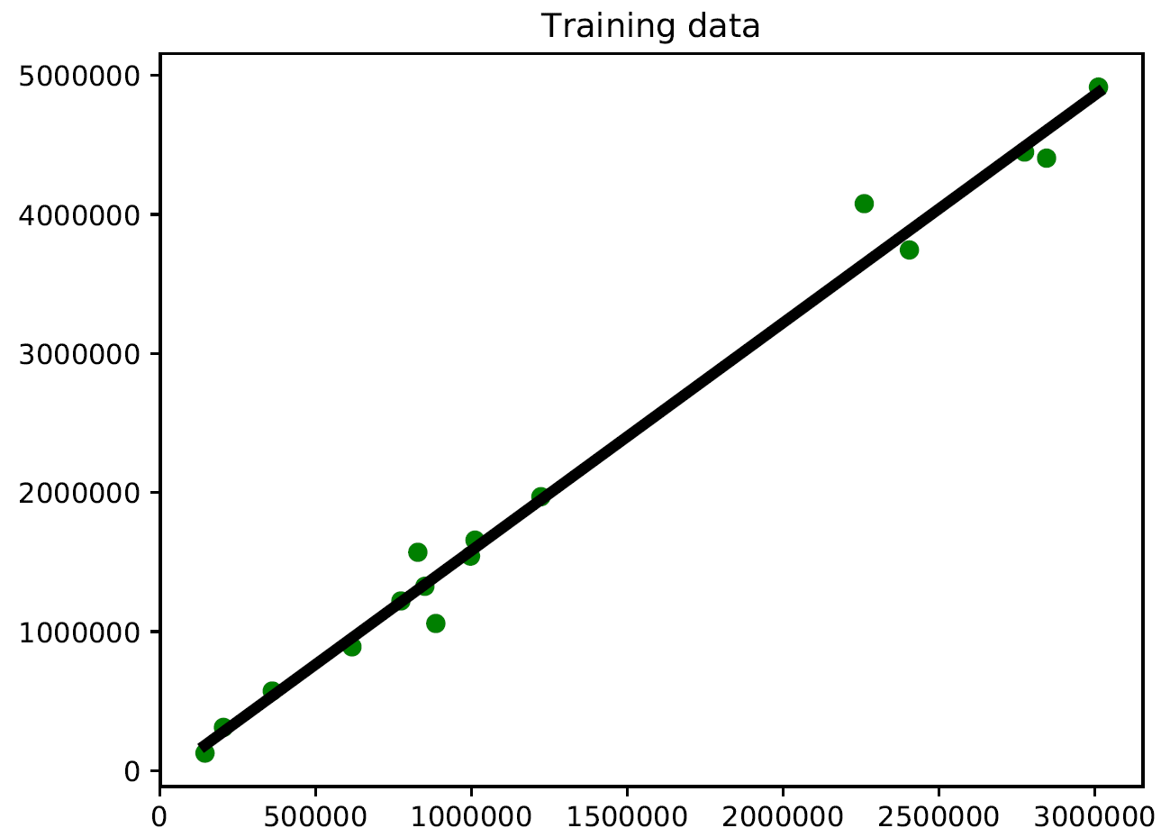
6. In the preceding code, we used the trained model to predict the output for our training data. This wouldn't tell us how the model performs on unknown data, because we are running it on the training data. This just gives us an idea of how the model fits on training data. Looks like it's doing okay, as you can see in the preceding diagram!
7. Let's predict the test dataset output based on this model and plot it, as follows:

y_test_pred = linear_regressor.predict(X_test)
plt.figure()
plt.scatter(X_test, y_test, color='green')
plt.plot(X_test, y_test_pred, color='black', linewidth=4)
plt.title('Test data')
plt.show()

When you run this in the Terminal, the following output is returned:

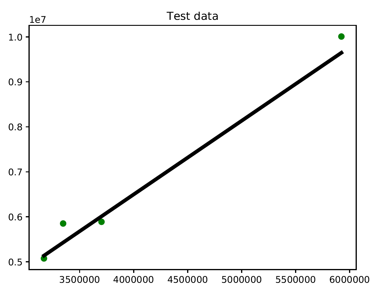
As you might expect, there's a positive association between a state's population and the number of vehicle registrations.

In this recipe, we looked for the linear regression relation between the vehicle registrations in a state and the population of a state. To do this we used the LinearRegression() function of the linear_model method of the sklearn library. After constructing the model, we first used the data involved in training the model to visually verify how well the model fits the data. Then, we used the test data to verify the results.

The best way to appreciate the results of a simulation is to display those using special charts. In fact, we have already used this technique in this section. I am referring to the chart in which we drew the scatter plot of the distribution with the regression line. In Chapter 5, Visualizing Data, we will see other plots that will allow us to check the model's hypotheses.

• Scikit-learn's official documentation of the sklearn.linear_model.LinearRegression() function: https://scikit-learn.org/stable/modules/generated/sklearn.linear_model.LinearRegression.html.
• Regression Analysis with R, Giuseppe Ciaburro, Packt Publishing.
• Linear regression: https://en.wikipedia.org/wiki/Linear_regression.
• Introduction to Linear Regression: http://onlinestatbook.com/2/regression/intro.html.

Now that we know how to build a regressor, it's important to understand how to evaluate the quality of a regressor as well. In this context, an error is defined as the difference between the actual value and the value that is predicted by the regressor.

Let's quickly take a look at the metrics that can be used to measure the quality of a regressor. A regressor can be evaluated using many different metrics. There is a module in the scikit-learn library that provides functionalities to compute all the following metrics. This is the sklearn.metrics module, which includes score functions, performance metrics, pairwise metrics, and distance computations.

Let's see how to compute regression accuracy in Python:

1. Now we will use the functions available to evaluate the performance of the linear regression model we developed in the previous recipe:

import sklearn.metrics as sm
print("Mean absolute error =", round(sm.mean_absolute_error(y_test, y_test_pred), 2)) 
print("Mean squared error =", round(sm.mean_squared_error(y_test, y_test_pred), 2)) 
print("Median absolute error =", round(sm.median_absolute_error(y_test, y_test_pred), 2)) 
print("Explain variance score =", round(sm.explained_variance_score(y_test, y_test_pred), 2)) 
print("R2 score =", round(sm.r2_score(y_test, y_test_pred), 2))

The following results are returned:

Mean absolute error = 241907.27
Mean squared error = 81974851872.13
Median absolute error = 240861.94
Explain variance score = 0.98
R2 score = 0.98

An R2 score near 1 means that the model is able to predict the data very well. Keeping track of every single metric can get tedious, so we pick one or two metrics to evaluate our model. A good practice is to make sure that the mean squared error is low and the explained variance score is high.

A regressor can be evaluated using many different metrics, such as the following:

• Mean absolute error: This is the average of absolute errors of all the data points in the given dataset.
• Mean squared error: This is the average of the squares of the errors of all the data points in the given dataset. It is one of the most popular metrics out there!
• Median absolute error: This is the median of all the errors in the given dataset. The main advantage of this metric is that it's robust to outliers. A single bad point in the test dataset wouldn't skew the entire error metric, as opposed to a mean error metric.
• Explained variance score: This score measures how well our model can account for the variation in our dataset. A score of 1.0 indicates that our model is perfect.
• R2 score: This is pronounced as R-squared, and this score refers to the coefficient of determination. This tells us how well the unknown samples will be predicted by our model. The best possible score is 1.0, but the score can be negative as well.

The sklearn.metrics module contains a series of simple functions that measure prediction error:

• Functions ending with _score return a value to maximize; the higher the better
• Functions ending with _error or _loss return a value to minimize; the lower the better

• Scikit-learn's official documentation of the sklearn.metrics module: https://scikit-learn.org/stable/modules/classes.html#module-sklearn.metrics.
• Regression Analysis with R, Giuseppe Ciaburro, Packt Publishing.

When we train a model, it would be nice if we could save it as a file so that it can be used later by simply loading it again.

Let's see how to achieve model persistence programmatically. To do this, the pickle module can be used. The pickle module is used to store Python objects. This module is a part of the standard library with your installation of Python.

Let's see how to achieve model persistence in Python:

1. Add the following lines to the regressor.py file:

import pickle

output_model_file = "3_model_linear_regr.pkl"

with open(output_model_file, 'wb') as f:
    pickle.dump(linear_regressor, f) 

2. The regressor object will be saved in the saved_model.pkl file. Let's look at how to load it and use it, as follows:

with open(output_model_file, 'rb') as f:
    model_linregr = pickle.load(f)

y_test_pred_new = model_linregr.predict(X_test)
print("New mean absolute error =", round(sm.mean_absolute_error(y_test, y_test_pred_new), 2))

The following result is returned:

New mean absolute error = 241907.27

Here, we just loaded the regressor from the file into the model_linregr variable. You can compare the preceding result with the earlier result to confirm that it's the same.

The pickle module transforms an arbitrary Python object into a series of bytes. This process is also called the serialization of the object. The byte stream representing the object can be transmitted or stored, and subsequently rebuilt to create a new object with the same characteristics. The inverse operation is called unpickling.

In Python, there is also another way to perform serialization, by using the marshal module. In general, the pickle module is recommended for serializing Python objects. The marshal module can be used to support Python .pyc files.

• Python's official documentation of the pickle module: https://docs.python.org/3/library/pickle.html

One of the main problems of linear regression is that it's sensitive to outliers. During data collection in the real world, it's quite common to wrongly measure output. Linear regression uses ordinary least squares, which tries to minimize the squares of errors. The outliers tend to cause problems because they contribute a lot to the overall error. This tends to disrupt the entire model.

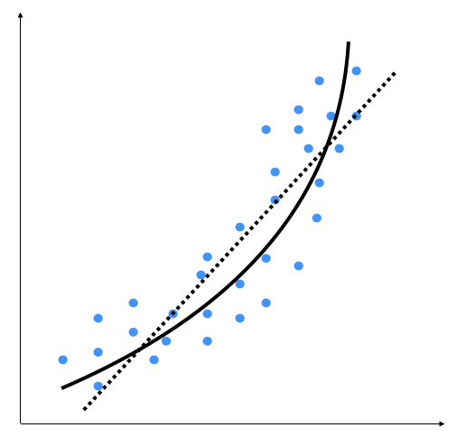
Let's try to deepen our understanding of the concept of outliers: outliers are values that, compared to others, are particularly extreme (values that are clearly distant from the other observations). Outliers are an issue because they might distort data analysis results; more specifically, descriptive statistics and correlations. We need to find these in the data cleaning phase, however, we can also get started on them in the next stage of data analysis. Outliers can be univariate when they have an extreme value for a single variable, or multivariate when they have a unique combination of values for a number of variables. Let's consider the following diagram:

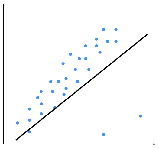
The two points on the bottom right are clearly outliers, but this model is trying to fit all the points. Hence, the overall model tends to be inaccurate. Outliers are the extreme values of a distribution that are characterized by being extremely high or extremely low compared to the rest of the distribution, and thus representing isolated cases with respect to the rest of the distribution. By visual inspection, we can see that the following output is a better model:

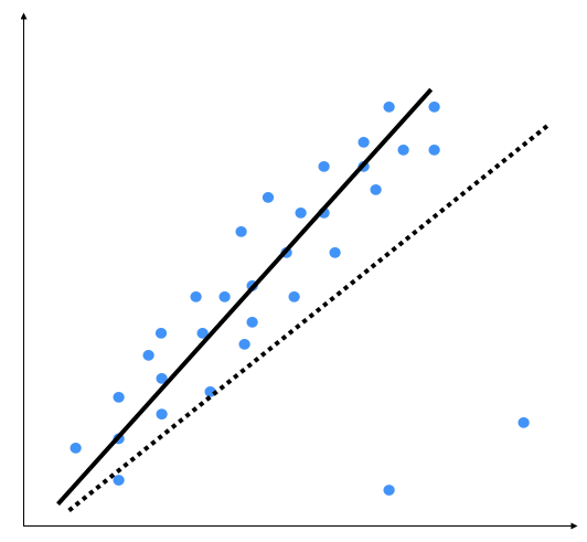
Ordinary least squares considers every single data point when it's building the model. Hence, the actual model ends up looking like the dotted line shown in the preceding graph. We can clearly see that this model is suboptimal.

The regularization method involves modifying the performance function, normally selected as the sum of the squares of regression errors on the training set. When a large number of variables are available, the least square estimates of a linear model often have a low bias but a high variance with respect to models with fewer variables. Under these conditions, there is an overfitting problem. To improve precision prediction by allowing greater bias but a small variance, we can use variable selection methods and dimensionality reduction, but these methods may be unattractive for computational burdens in the first case or provide a difficult interpretation in the other case.

Another way to address the problem of overfitting is to modify the estimation method by neglecting the requirement of an unbiased parameter estimator and instead considering the possibility of using a biased estimator, which may have smaller variance. There are several biased estimators, most of which are based on regularization: Ridge, Lasso, and ElasticNet are the most popular methods.

Ridge regression is a regularization method where a penalty is imposed on the size of the coefficients. As we said in the Building a linear regressor section, in the ordinary least squares method, the coefficients are estimated by determining numerical values that minimize the sum of the squared deviations between the observed responses and the fitted responses, according to the following equation:

Ridge regression, in order to estimate the β coefficients, starts from the basic formula of the residual sum of squares (RSS) and adds the penalty term. λ (≥ 0) is defined as the tuning parameter, which is multiplied by the sum of the β coefficients squared (excluding the intercept) to define the penalty period, as shown in the following equation:

It is evident that having λ = 0 means not having a penalty in the model, that is, we would produce the same estimates as the least squares. On the other hand, having a λ tending toward infinity means having a high penalty effect, which will bring many coefficients close to zero, but will not imply their exclusion from the model. Let's see how to build a ridge regressor in Python.

Let's see how to build a ridge regressor in Python:

1. You can use the data already used in the previous example: Building a linear regressor (VehiclesItaly.txt). This file contains two values in each line. The first value is the explanatory variable, and the second is the response variable.
2. Add the following lines to regressor.py. Let's initialize a ridge regressor with some parameters:

from sklearn import linear_model
ridge_regressor = linear_model.Ridge(alpha=0.01, fit_intercept=True, max_iter=10000)

3. The alpha parameter controls the complexity. As alpha gets closer to 0, the ridge regressor tends to become more like a linear regressor with ordinary least squares. So, if you want to make it robust against outliers, you need to assign a higher value to alpha. We considered a value of 0.01, which is moderate.
4. Let's train this regressor, as follows:

ridge_regressor.fit(X_train, y_train)
y_test_pred_ridge = ridge_regressor.predict(X_test)
print( "Mean absolute error =", round(sm.mean_absolute_error(y_test, y_test_pred_ridge), 2))
print( "Mean squared error =", round(sm.mean_squared_error(y_test, y_test_pred_ridge), 2))
print( "Median absolute error =", round(sm.median_absolute_error(y_test, y_test_pred_ridge), 2))
print( "Explain variance score =", round(sm.explained_variance_score(y_test, y_test_pred_ridge), 2))
print( "R2 score =", round(sm.r2_score(y_test, y_test_pred_ridge), 2))

Run this code to view the error metrics. You can build a linear regressor to compare and contrast the results on the same data to see the effect of introducing regularization into the model.

Ridge regression is a regularization method where a penalty is imposed on the size of the coefficients. Ridge regression is identical to least squares, barring the fact that ridge coefficients are computed by decreasing a quantity that is somewhat different. In ridge regression, a scale transformation has a substantial effect. Therefore, to avoid obtaining different results depending on the predicted scale of measurement, it is advisable to standardize all predictors before estimating the model. To standardize the variables, we must subtract their means and divide by their standard deviations.

• Scikit-learn's official documentation of the linear_model.Ridge function: https://scikit-learn.org/stable/modules/generated/sklearn.linear_model.Ridge.html
• Ridge Regression, Columbia University: https://www.mailman.columbia.edu/research/population-health-methods/ridge-regression
• Multicollinearity and Other Regression Pitfalls, The Pennsylvania State University: https://newonlinecourses.science.psu.edu/stat501/node/343/

One of the main constraints of a linear regression model is the fact that it tries to fit a linear function to the input data. The polynomial regression model overcomes this issue by allowing the function to be a polynomial, thereby increasing the accuracy of the model.

Polynomial models should be applied where the relationship between response and explanatory variables is curvilinear. Sometimes, polynomial models can also be used to model a non-linear relationship in a small range of explanatory variable. A polynomial quadratic (squared) or cubic (cubed) term converts a linear regression model into a polynomial curve. However, since it is the explanatory variable that is squared or cubed and not the beta coefficient, it is still considered as a linear model. This makes it a simple and easy way to model curves, without needing to create big non-linear models. Let's consider the following diagram:

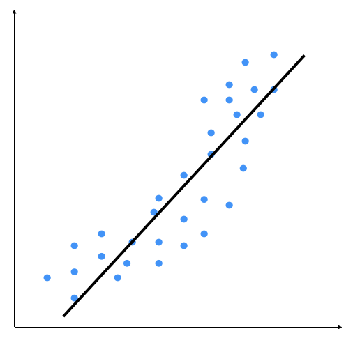
We can see that there is a natural curve to the pattern of data points. This linear model is unable to capture this. Let's see what a polynomial model would look like:

The dotted line represents the linear regression model, and the solid line represents the polynomial regression model. The curviness of this model is controlled by the degree of the polynomial. As the curviness of the model increases, it gets more accurate. However, curviness adds complexity to the model as well, making it slower. This is a trade-off: you have to decide how accurate you want your model to be given the computational constraints.

Let's see how to build a polynomial regressor in Python:

1. In this example, we will only deal with second-degree parabolic regression. Now, we'll show how to model data with a polynomial. We measured the temperature for a few hours of the day. We want to know the temperature trend even at times of the day when we did not measure it. Those times are, however, between the initial time and the final time at which our measurements took place:

import numpy as np

Time = np.array([6, 8, 11, 14, 16, 18, 19])
Temp = np.array([4, 7, 10, 12, 11.5, 9, 7])

2. Now, we will show the temperature at a few points during the day:

import matplotlib.pyplot as plt
plt.figure()
plt.plot(Time, Temp, 'bo')
plt.xlabel("Time")
plt.ylabel("Temp")
plt.title('Temperature versus time')
plt.show()

The following graph is produced:

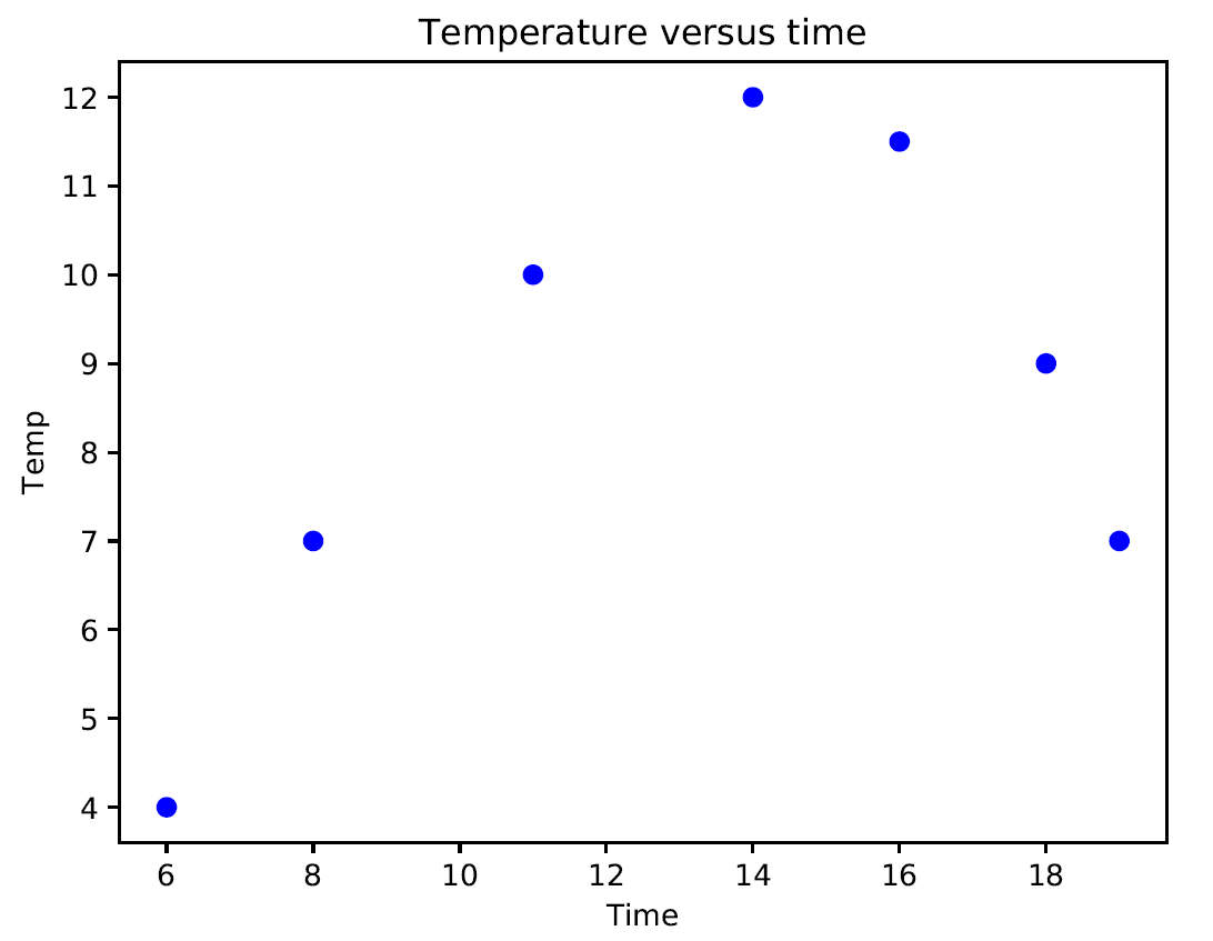
If we analyze the graph, it is possible to note a curvilinear pattern of the data that can be modeled through a second-degree polynomial such as the following equation:

The unknown coefficients, β₀, β₁, and β₂, are estimated by decreasing the value of the sum of the squares. This is obtained by minimizing the deviations of the data from the model to its lowest value (least squares fit).

3. Let's calculate the polynomial coefficients:

beta = np.polyfit(Time, Temp, 2)

The numpy.polyfit() function returns the coefficients for a polynomial of degree n (given by us) that is the best fit for the data. The coefficients returned by the function are in descending powers (highest power first), and their length is n+1 if n is the degree of the polynomial.

4. After creating the model, let's verify that it actually fits our data. To do this, use the model to evaluate the polynomial at uniformly spaced times. To evaluate the model at the specified points, we can use the poly1d() function. This function returns the value of a polynomial of degree n evaluated at the points provided by us. The input argument is a vector of length n+1 whose elements are the coefficients in descending powers of the polynomial to be evaluated:

p = np.poly1d(beta)

As you can see in the upcoming graph, this is close to the output value. If we want it to get closer, we need to increase the degree of the polynomial.

5. Now we can plot the original data and the model on the same plot:

xp = np.linspace(6, 19, 100)
plt.figure()
plt.plot(Time, Temp, 'bo', xp, p(xp), '-')
plt.show()

The following graph is printed:

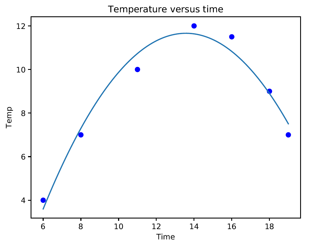
If we analyze the graph, we can see that the curve fits our data sufficiently. This model fits the data to a greater extent than a simple linear regression model. In regression analysis, it's important to keep the order of the model as low as possible. In the first analysis, we keep the model as a first order polynomial. If this is not satisfactory, then a second-order polynomial is tried. The use of higher-order polynomials can lead to incorrect evaluations.

Polynomial regression should be used when linear regression is not good enough. With polynomial regression, we approached a model in which some predictors appear in degrees equal to or greater than two to fit the data with a curved line. Polynomial regression is usually used when the relationship between variables looks curved.

At what degree of the polynomial must we stop? It depends on the degree of precision we are looking for. The higher the degree of the polynomial, the greater the precision of the model, but the more difficult it is to calculate. In addition, it is necessary to verify the significance of the coefficients that are found, but let's get to it right away.

• Python's official documentation of the numpy.polyfit() function (https://docs.scipy.org/doc/numpy/reference/generated/numpy.polyfit.html)
• Python's official documentation of the numpy.poly1d() function (https://docs.scipy.org/doc/numpy-1.14.0/reference/generated/numpy.poly1d.html)

It's time to apply our knowledge to a real-world problem. Let's apply all these principles to estimate house prices. This is one of the most popular examples that is used to understand regression, and it serves as a good entry point. This is intuitive and relatable, hence making it easier to understand the concepts before we perform more complex things in machine learning. We will use a decision tree regressor with AdaBoost to solve this problem.

A decision tree is a tree where each node makes a simple decision that contributes to the final output. The leaf nodes represent the output values, and the branches represent the intermediate decisions that were made, based on input features. AdaBoost stands for adaptive boosting, and this is a technique that is used to boost the accuracy of the results from another system. This combines the outputs from different versions of the algorithms, called weak learners, using a weighted summation to get the final output. The information that's collected at each stage of the AdaBoost algorithm is fed back into the system so that the learners at the latter stages focus on training samples that are difficult to classify. In this way, it increases the accuracy of the system.

Using AdaBoost, we fit a regressor on the dataset. We compute the error and then fit the regressor on the same dataset again, based on this error estimate. We can think of this as fine-tuning of the regressor until the desired accuracy is achieved. You are given a dataset that contains various parameters that affect the price of a house. Our goal is to estimate the relationship between these parameters and the house price so that we can use this to estimate the price given unknown input parameters.

Let's see how to estimate housing prices in Python:

1. Create a new file called housing.py and add the following lines:

import numpy as np
from sklearn.tree import DecisionTreeRegressor
from sklearn.ensemble import AdaBoostRegressor
from sklearn import datasets
from sklearn.metrics import mean_squared_error, explained_variance_score
from sklearn.utils import shuffle
import matplotlib.pyplot as plt

2. There is a standard housing dataset that people tend to use to get started with machine learning. You can download it at https://archive.ics.uci.edu/ml/machine-learning-databases/housing/. We will be using a slightly modified version of the dataset, which has been provided along with the code files.
   The good thing is that scikit-learn provides a function to directly load this dataset:

housing_data = datasets.load_boston()

Each data point has 12 input parameters that affect the price of a house. You can access the input data using housing_data.data and the corresponding price using housing_data.target. The following attributes are available:

• crim: Per capita crime rate by town
• zn: Proportion of residential land zoned for lots that are over 25,000 square feet
• indus: Proportion of non-retail business acres per town
• chas: Charles River dummy variable (= 1 if tract bounds river; 0 otherwise)
• nox: Nitric oxides concentration (parts per ten million)
• rm: Average number of rooms per dwelling
• age: Proportion of owner-occupied units built prior to 1940
• dis: Weighted distances to the five Boston employment centers
• rad: Index of accessibility to radial highways
• tax: Full-value property-tax rate per $10,000
• ptratio: Pupil-teacher ratio by town
• lstat: Percent of the lower status of the population
• target: Median value of owner-occupied homes in $1000

Of these, target is the response variable, while the other 12 variables are possible predictors. The goal of this analysis is to fit a regression model that best explains the variation in target.

3. Let's separate this into input and output. To make this independent of the ordering of the data, let's shuffle it as well:

X, y = shuffle(housing_data.data, housing_data.target, random_state=7)

The sklearn.utils.shuffle() function shuffles arrays or sparse matrices in a consistent way to do random permutations of collections. Shuffling data reduces variance and makes sure that the patterns remain general and less overfitted. The random_state parameter controls how we shuffle data so that we can have reproducible results.

4. Let's divide the data into training and testing. We'll allocate 80% for training and 20% for testing:

num_training = int(0.8 * len(X))
X_train, y_train = X[:num_training], y[:num_training]
X_test, y_test = X[num_training:], y[num_training:]

Remember, machine learning algorithms, train models by using a finite set of training data. In the training phase, the model is evaluated based on its predictions of the training set. But the goal of the algorithm is to produce a model that predicts previously unseen observations, in other words, one that is able to generalize the problem by starting from known data and unknown data. For this reason, the data is divided into two datasets: training and test. The training set is used to train the model, while the test set is used to verify the ability of the system to generalize.

5. We are now ready to fit a decision tree regression model. Let's pick a tree with a maximum depth of 4, which means that we are not letting the tree become arbitrarily deep:

dt_regressor = DecisionTreeRegressor(max_depth=4)
dt_regressor.fit(X_train, y_train)

The DecisionTreeRegressor function has been used to build a decision tree regressor.

6. Let's also fit the decision tree regression model with AdaBoost:

ab_regressor = AdaBoostRegressor(DecisionTreeRegressor(max_depth=4), n_estimators=400, random_state=7)
ab_regressor.fit(X_train, y_train)

The AdaBoostRegressor function has been used to compare the results and see how AdaBoost really boosts the performance of a decision tree regressor.

7. Let's evaluate the performance of the decision tree regressor:

y_pred_dt = dt_regressor.predict(X_test)
mse = mean_squared_error(y_test, y_pred_dt)
evs = explained_variance_score(y_test, y_pred_dt)
print("#### Decision Tree performance ####")
print("Mean squared error =", round(mse, 2))
print("Explained variance score =", round(evs, 2))

First, we used the predict() function to predict the response variable based on the test data. Next, we calculated mean squared error and explained variance. Mean squared error is the average of the squared difference between actual and predicted values across all data points in the input. The explained variance is an indicator that, in the form of proportion, indicates how much variability of our data is explained by the model in question.

8. Now, let's evaluate the performance of AdaBoost:

y_pred_ab = ab_regressor.predict(X_test)
mse = mean_squared_error(y_test, y_pred_ab)
evs = explained_variance_score(y_test, y_pred_ab)
print("#### AdaBoost performance ####")
print("Mean squared error =", round(mse, 2))
print("Explained variance score =", round(evs, 2))

Here is the output on the Terminal:

#### Decision Tree performance ####
Mean squared error = 14.79
Explained variance score = 0.82

#### AdaBoost performance ####
Mean squared error = 7.54
Explained variance score = 0.91

The error is lower and the variance score is closer to 1 when we use AdaBoost, as shown in the preceding output.

DecisionTreeRegressor builds a decision tree regressor. Decision trees are used to predict a response or class y, from several input variables; x1, x2,…,xn. If y is a continuous response, it's called a regression tree, if y is categorical, it's called a classification tree. The algorithm is based on the following procedure: We see the value of the input x_i at each node of the tree, and based on the answer, we continue to the left or to the right branch. When we reach a leaf, we will find the prediction. In regression trees, we try to divide the data space into tiny parts, where we can equip a simple different model on each of them. The non-leaf part of the tree is just the way to find out which model we will use for predicting it.

A regression tree is formed by a series of nodes that split the root branch into two child branches. Such subdivision continues to cascade. Each new branch, then, can go in another node, or remain a leaf with the predicted value.

An AdaBoost regressor is a meta-estimator that starts by equipping a regressor on the actual dataset and adding additional copies of the regressor on the same dataset, but where the weights of instances are adjusted according to the error of the current prediction. As such, consecutive regressors look at difficult cases. This will help us compare the results and see how AdaBoost really boosts the performance of a decision tree regressor.

• Scikit-learn's official documentation of the DecisionTreeRegressor function (https://scikit-learn.org/stable/modules/generated/sklearn.tree.DecisionTreeRegressor.html)
• Scikit-learn's official documentation of the AdaBoostRegressor function (https://scikit-learn.org/stable/modules/generated/sklearn.ensemble.AdaBoostRegressor.html)

Are all features equally important? In this case, we used 13 input features, and they all contributed to the model. However, an important question here is, How do we know which features are more important? Obviously, not all features contribute equally to the output. In case we want to discard some of them later, we need to know which features are less important. We have this functionality available in scikit-learn.

Let's calculate the relative importance of the features. Feature importance provides a measure that indicates the value of each feature in the construction of the model. The more an attribute is used to build the model, the greater its relative importance. This importance is explicitly calculated for each attribute in the dataset, allowing you to classify and compare attributes to each other. Feature importance is an attribute contained in the model (feature_importances_).

Let's see how to compute the relative importance of features:

1. Let's see how to extract this. Add the following lines to housing.py:

DTFImp= dt_regressor.feature_importances_
DTFImp= 100.0 * (DTFImp / max(DTFImp))
index_sorted = np.flipud(np.argsort(DTFImp))
pos = np.arange(index_sorted.shape[0]) + 0.5

The regressor object has a callable feature_importances_ method that gives us the relative importance of each feature. To compare the results, the importance values have been normalized. Then, we ordered the index values and turned them upside down so that they are arranged in descending order of importance. Finally, for display purposes, the location of the labels on the x-axis has been centered.

2. To visualize the results, we will plot the bar graph:

plt.figure()
plt.bar(pos, DTFImp[index_sorted], align='center')
plt.xticks(pos, housing_data.feature_names[index_sorted])
plt.ylabel('Relative Importance')
plt.title("Decision Tree regressor")
plt.show()

3. We just take the values from the feature_importances_ method and scale them so that they range between 0 and 100. Let's see what we will get for a decision tree-based regressor in the following output:

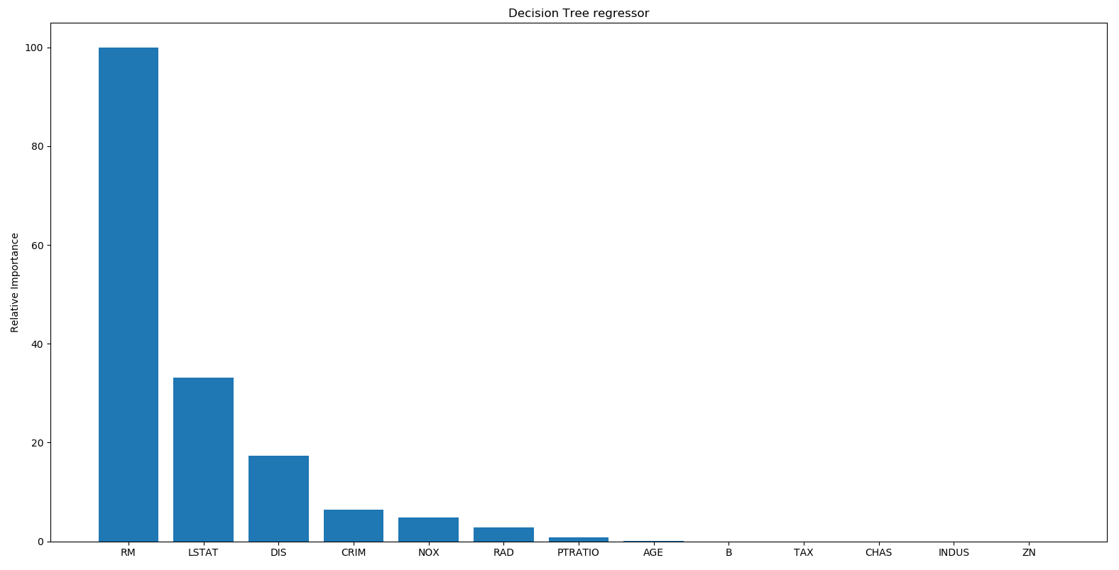
So, the decision tree regressor says that the most important feature is RM.

4. Now, we carry out a similar procedure for the AdaBoost model:

ABFImp= ab_regressor.feature_importances_ 
ABFImp= 100.0 * (ABFImp / max(ABFImp))
index_sorted = np.flipud(np.argsort(ABFImp))
pos = np.arange(index_sorted.shape[0]) + 0.5

5. To visualize the results, we will plot the bar graph:

plt.figure()
plt.bar(pos, ABFImp[index_sorted], align='center')
plt.xticks(pos, housing_data.feature_names[index_sorted])
plt.ylabel('Relative Importance')
plt.title("AdaBoost regressor")
plt.show()

Let's take a look at what AdaBoost has to say in the following output:

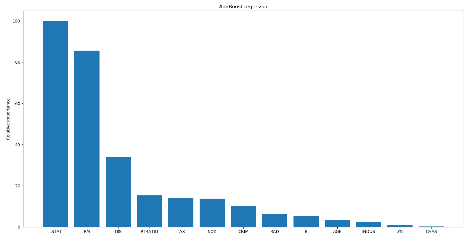
According to AdaBoost, the most important feature is LSTAT. In reality, if you build various regressors on this data, you will see that the most important feature is in fact LSTAT. This shows the advantage of using AdaBoost with a decision tree-based regressor.

Feature importance provides a measure that indicates the value of each feature in the construction of a model. The more an attribute is used to build a model, the greater its relative importance. In this recipe, the feature_importances_ attribute was used to extract the relative importance of the features from the model.

Relative importance returns the utility of each characteristic in the construction of decision trees. The more an attribute is used to make predictions with decision trees, the greater its relative importance. This importance is explicitly calculated for each attribute in the dataset, allowing you to classify and compare attributes to each other.

• Scikit-learn's official documentation of the DecisionTreeRegressor function: https://scikit-learn.org/stable/modules/generated/sklearn.tree.DecisionTreeRegressor.html

Let's use a different regression method to solve the bicycle demand distribution problem. We will use the random forest regressor to estimate the output values. A random forest is a collection of decision trees. This basically uses a set of decision trees that are built using various subsets of the dataset, and then it uses averaging to improve the overall performance.

We will use the bike_day.csv file that is provided to you. This is also available at https://archive.ics.uci.edu/ml/datasets/Bike+Sharing+Dataset. There are 16 columns in this dataset. The first two columns correspond to the serial number and the actual date, so we won't use them for our analysis. The last three columns correspond to different types of outputs. The last column is just the sum of the values in the fourteenth and fifteenth columns, so we can leave those two out when we build our model. Let's go ahead and see how to do this in Python. We will analyze the code line by line to understand each step.

Let's see how to estimate bicycle demand distribution:

1. We first need to import a couple of new packages, as follows:

import csv
import numpy as np

2. We are processing a CSV file, so the CSV package for useful in handling these files. Let's import the data into the Python environment:

filename="bike_day.csv"
file_reader = csv.reader(open(filename, 'r'), delimiter=',')
X, y = [], []
for row in file_reader:
    X.append(row[2:13])
    y.append(row[-1])

This piece of code just read all the data from the CSV file. The csv.reader() function returns a reader object, which will iterate over lines in the given CSV file. Each row read from the CSV file is returned as a list of strings. So, two lists are returned: X and y. We have separated the data from the output values and returned them. Now we will extract feature names:

feature_names = np.array(X[0])

The feature names are useful when we display them on a graph. So, we have to remove the first row from X and y because they are feature names:

X=np.array(X[1:]).astype(np.float32)
y=np.array(y[1:]).astype(np.float32)

We have also converted the two lists into two arrays.

3. Let's shuffle these two arrays to make them independent of the order in which the data is arranged in the file:

from sklearn.utils import shuffle
X, y = shuffle(X, y, random_state=7)  

4. As we did earlier, we need to separate the data into training and testing data. This time, let's use 90% of the data for training and the remaining 10% for testing:

num_training = int(0.9 * len(X))
X_train, y_train = X[:num_training], y[:num_training]
X_test, y_test = X[num_training:], y[num_training:]

5. Let's go ahead and train the regressor:

from sklearn.ensemble import RandomForestRegressor
rf_regressor = RandomForestRegressor(n_estimators=1000, max_depth=10, min_samples_split=2)
rf_regressor.fit(X_train, y_train)

The RandomForestRegressor() function builds a random forest regressor. Here, n_estimators refers to the number of estimators, which is the number of decision trees that we want to use in our random forest. The max_depth parameter refers to the maximum depth of each tree, and the min_samples_split parameter refers to the number of data samples that are needed to split a node in the tree.

6. Let's evaluate the performance of the random forest regressor:

y_pred = rf_regressor.predict(X_test)
from sklearn.metrics import mean_squared_error, explained_variance_score
mse = mean_squared_error(y_test, y_pred)
evs = explained_variance_score(y_test, y_pred)
print( "#### Random Forest regressor performance ####")
print("Mean squared error =", round(mse, 2))
print("Explained variance score =", round(evs, 2))

The following results are returned:

#### Random Forest regressor performance ####
Mean squared error = 357864.36
Explained variance score = 0.89

7. Let's extract the relative importance of the features:

RFFImp= rf_regressor.feature_importances_ 
RFFImp= 100.0 * (RFFImp / max(RFFImp))
index_sorted = np.flipud(np.argsort(RFFImp))
pos = np.arange(index_sorted.shape[0]) + 0.5

To visualize the results, we will plot a bar graph:

import matplotlib.pyplot as plt
plt.figure()
plt.bar(pos, RFFImp[index_sorted], align='center')
plt.xticks(pos, feature_names[index_sorted])
plt.ylabel('Relative Importance')
plt.title("Random Forest regressor")
plt.show()

The following output is plotted:

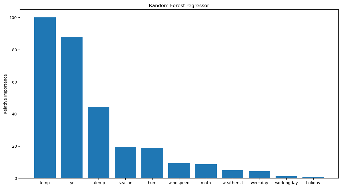
Looks like the temperature is the most important factor controlling bicycle rentals.

A random forest is a special regressor formed of a set of simple regressors (decision trees), represented as independent and identically distributed random vectors, where each one chooses the mean prediction of the individual trees. This type of structure has made significant improvements in regression accuracy and falls within the sphere of ensemble learning. Each tree within a random forest is constructed and trained from a random subset of the data in the training set. The trees therefore do not use the complete set, and the best attribute is no longer selected for each node, but the best attribute is selected from a set of randomly selected attributes.

Randomness is a factor that then becomes part of the construction of regressors and aims to increase their diversity and thus reduce correlation. The final result returned by the random forest is nothing but the average of the numerical result returned by the different trees in the case of a regression, or the class returned by the largest number of trees if the random forest algorithm was used to perform classification.

Let's see what happens when you include the fourteenth and fifteenth columns in the dataset. In the feature importance graph, every feature other than these two has to go to zero. The reason is that the output can be obtained by simply summing up the fourteenth and fifteenth columns, so the algorithm doesn't need any other features to compute the output. Make the following change inside the for loop (the rest of the code remains unchanged):

X.append(row[2:15])

If you plot the feature importance graph now, you will see the following:

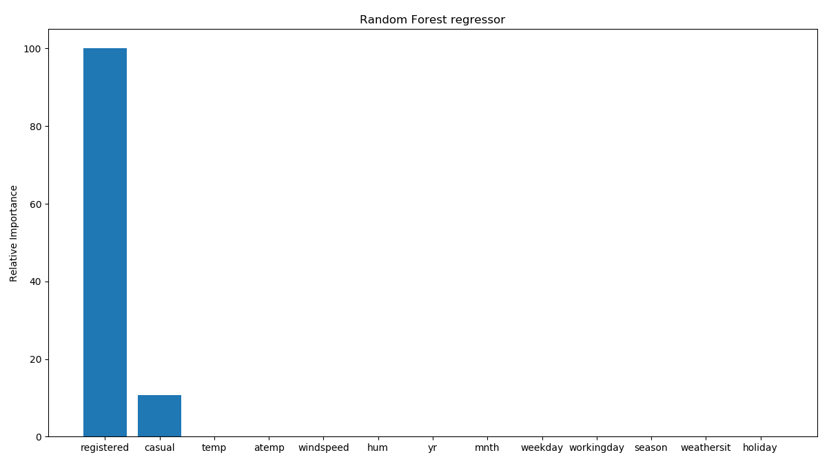
As expected, it says that only these two features are important. This makes sense intuitively because the final output is a simple summation of these two features. So, there is a direct relationship between these two variables and the output value. Hence, the regressor says that it doesn't need any other variable to predict the output. This is an extremely useful tool to eliminate redundant variables in your dataset. But this is not the only difference from the previous model. If we analyze the model's performance, we can see a substantial improvement:

#### Random Forest regressor performance ####
Mean squared error = 22552.26
Explained variance score = 0.99

We therefore have 99% of the variance explained: a very good result.

There is another file, called bike_hour.csv, that contains data about how the bicycles are shared hourly. We need to consider columns 3 to 14, so let's make this change in the code (the rest of the code remains unchanged):

filename="bike_hour.csv"
file_reader = csv.reader(open(filename, 'r'), delimiter=',')
X, y = [], []
for row in file_reader:
    X.append(row[2:14])
    y.append(row[-1])

If you run the new code, you will see the performance of the regressor displayed, as follows:

#### Random Forest regressor performance ####
Mean squared error = 2613.86
Explained variance score = 0.92

The feature importance graph will look like the following:

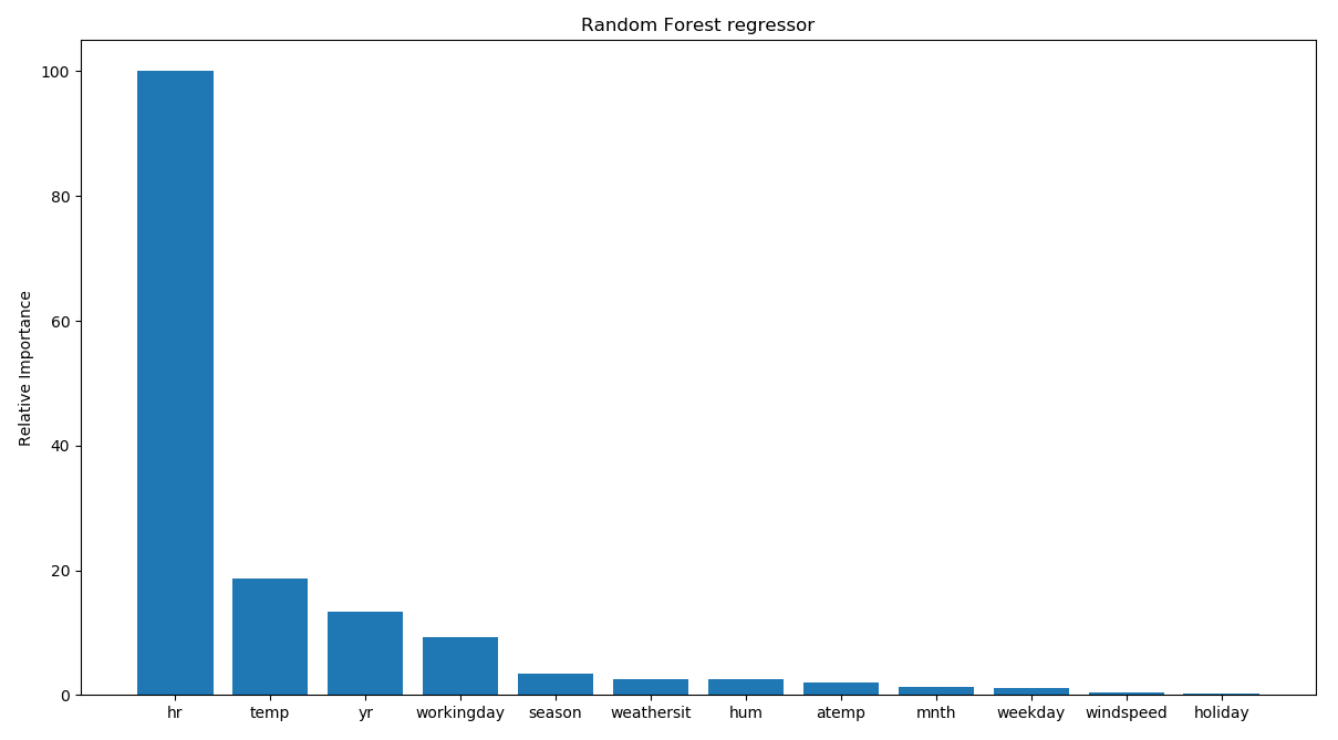
This shows that the hour of the day is the most important feature, which makes sense intuitively if you think about it! The next important feature is temperature, which is consistent with our earlier analysis.

• Scikit-learn's official documentation of the RandomForestRegressor function: https://scikit-learn.org/stable/modules/generated/sklearn.ensemble.RandomForestRegressor.html