The term Numerical Linear Algebra refers to the use of matrices to solve computational science problems. In this chapter, we start by learning how to construct these objects effectively in Python. We make an emphasis on importing large sparse matrices from repositories online. We then proceed to reviewing basic manipulation and operations on them. The next step is a study of the different matrix functions implemented in SciPy. We continue on to exploring different factorizations for the solution of matrix equations, and for the computation of eigenvalues and their corresponding eigenvectors.
The following image shows a graph that represents a series of web pages (numbered from 1 to 8):
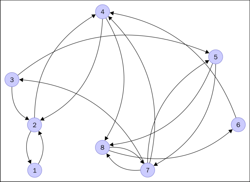
An arrow from a node to another indicates the existence of a link from the web page, represented by the sending node, to the page represented by the receiving node. For example, the arrow from node 2 to node 1 indicates that there is a link in web page 2 pointing to web page 1. Notice how web page 4 has two outer links (to pages 2 and 8), and there are three pages that link to web page 4 (pages 2, 6, and 7). The pages represented by nodes 2, 4, and 8 seem to be the most popular at first sight.
Is there a mathematical way to actually express the popularity of a web page within a network? Researchers at Google came up with the idea of a PageRank to roughly estimate this concept by counting the number and quality of links to a page. It goes like this:
We construct a transition matrix of this graph,
T={a[i,j]}, in the following fashion: the entrya[i,j]is1/kif there is a link from web pageito web pagej, and the total number of outer links in web pageiamounts tok. Otherwise, the entry is just zero. The size of a transition matrix of N web pages is always N × N. In our case, the matrix has size 8 × 8:0 1/2 0 0 0 0 0 0 1 0 1/2 1/2 0 0 0 0 0 0 0 0 0 0 1/3 0 0 1/2 0 0 0 1 1/3 0 0 0 1/2 0 0 0 0 0 0 0 0 0 0 0 0 1/2 0 0 0 0 1/2 0 0 1/2 0 0 0 1/2 1/2 0 1/3 0
Let us open an iPython session and load this particular matrix to memory.
In [1]: import numpy as np, matplotlib.pyplot as plt, \
   ...: scipy.linalg as spla, scipy.sparse as spsp, \
   ...: scipy.sparse.linalg as spspla
In [2]: np.set_printoptions(suppress=True, precision=3)
In [3]: cols = np.array([0,1,1,2,2,3,3,4,4,5,6,6,6,7,7]); \
   ...: rows = np.array([1,0,3,1,4,1,7,6,7,3,2,3,7,5,6]); \
   ...: data = np.array([1., 0.5, 0.5, 0.5, 0.5, \
   ...:                  0.5, 0.5, 0.5, 0.5, 1., \
   ...:                  1./3, 1./3, 1./3, 0.5, 0.5])
In [4]: T = np.zeros((8,8)); \
   ...: T[rows,cols] = data
From the transition matrix, we create a PageRank matrix G by fixing a positive constant p between 0 and 1, and following the formula G = (1-p)*T + p*B for a suitable damping factor p. Here, B is a matrix with the same size as T, with all its entries equal to 1/N. For example, if we choose p = 0.15, we obtain the following PageRank matrix:
In [5]: G = (1-0.15) * T + 0.15/8; \
   ...: print G
[[ 0.019  0.444  0.019  0.019  0.019  0.019  0.019  0.019]
 [ 0.869  0.019  0.444  0.444  0.019  0.019  0.019  0.019]
 [ 0.019  0.019  0.019  0.019  0.019  0.019  0.302  0.019]
 [ 0.019  0.444  0.019  0.019  0.019  0.869  0.302  0.019]
 [ 0.019  0.019  0.444  0.019  0.019  0.019  0.019  0.019]
 [ 0.019  0.019  0.019  0.019  0.019  0.019  0.019  0.444]
 [ 0.019  0.019  0.019  0.019  0.444  0.019  0.019  0.444]
 [ 0.019  0.019  0.019  0.444  0.444  0.019  0.302  0.019]]
PageRank matrices have some interesting properties:
1 is an eigenvalue of multiplicity one.
1 is actually the largest eigenvalue; all the other eigenvalues are in modulus smaller than 1.
The eigenvector corresponding to eigenvalue 1 has all positive entries. In particular, for the eigenvalue 1, there exists a unique eigenvector with the sum of its entries equal to 1. This is what we call the
PageRankvector.
A quick computation with scipy.linalg.eig finds that eigenvector for us:
In [6]: eigenvalues, eigenvectors = spla.eig(G); \
   ...: print eigenvalues
[ 1.000+0.j    -0.655+0.j    -0.333+0.313j -0.333-0.313j –0.171+0.372j -0.171-0.372j  0.544+0.j     0.268+0.j   ]
In [7]: PageRank = eigenvectors[:,0]; \
   ...: PageRank /= sum(PageRank); \
   ...: print PageRank.real
[ 0.117  0.232  0.048  0.219  0.039  0.086  0.102  0.157]
Those values correspond to the PageRank of each of the eight web pages depicted on the graph. As expected, the maximum value of those is associated to the second web page (0.232), closely followed by the fourth (0.219) and then the eighth web page (0.157). These values provide us with the information that we were seeking: the second web page is the most popular, followed by the fourth, and then, the eight.
Note
Note how this problem of networks of web pages has been translated into mathematical objects, to an equivalent problem involving matrices, eigenvalues, and eigenvectors, and has been solved with techniques of Linear Algebra.
The transition matrix is sparse: most of its entries are zeros. Sparse matrices with an extremely large size are of special importance in Numerical Linear Algebra, not only because they encode challenging scientific problems but also because it is extremely hard to manipulate them with basic algorithms.
Rather than storing to memory all values in the matrix, it makes sense to collect only the non-zero values instead, and use algorithms which exploit these smart storage schemes. The gain in memory management is obvious. These methods are usually faster for this kind of matrices and give less roundoff errors, since there are usually far less operations involved. This is another advantage of SciPy, since it contains numerous procedures to attack different problems where data is stored in this fashion. Let us observe its power with another example:
The University of Florida Sparse Matrix Collection is the largest database of matrices accessible online. As of January 2014, it contains 157 groups of matrices arising from all sorts of scientific disciplines. The sizes of the matrices range from very small (1 × 2) to insanely large (28 million × 28 million). More matrices are expected to be added constantly, as they arise in different engineering problems.
Tip
More information about this database can be found in ACM Transactions on Mathematical Software, vol. 38, Issue 1, 2011, pp 1:1-1:25, by T.A. Davis and Y.Hu, or online at http://www.cise.ufl.edu/research/sparse/matrices/.
For example, the group with the most matrices in the database is the original Harwell-Boeing Collection, with 292 different sparse matrices. This group can also be accessed online at the Matrix Market: http://math.nist.gov/MatrixMarket/.
Each matrix in the database comes in three formats:
Let us import to our iPython session two matrices in the Matrix Market Exchange format from the collection, meant to be used in a solution of a least squares problem. These matrices are located at www.cise.ufl.edu/research/sparse/matrices/Bydder/mri2.html.The numerical values correspond to phantom data acquired on a Sonata 1.5-T scanner (Siemens, Erlangen, Germany) using a magnetic resonance imaging (MRI) device. The object measured is a simulation of a human head made with several metallic objects. We download the corresponding tar bundle and untar it to get two ASCII files:
mri2.mtx(the main matrix in the least squares problem)mri2_b.mtx(the right-hand side of the equation)
The first twenty lines of the file mri2.mtx read as follows:
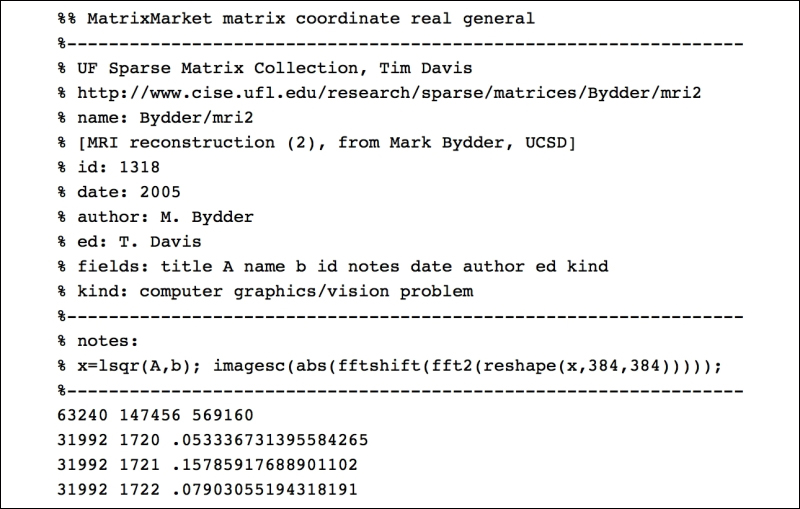
The first sixteen lines are comments, and give us some information about the generation of the matrix.
The computer vision problem where it arose: An MRI reconstruction
Author information: Mark Bydder, UCSD
Procedures to apply to the data: Solve a least squares problem A * x - b, and posterior visualization of the result
The seventeenth line indicates the size of the matrix, 63240 rows × 147456 columns, as well as the number of non-zero entries in the data, 569160.
The rest of the file includes precisely 569160 lines, each containing two integer numbers, and a floating point number: These are the locations of the non-zero elements in the matrix, together with the corresponding values.
Tip
We need to take into account that these files use the FORTRAN convention of starting arrays from 1, not from 0.
A good way to read this file into ndarray is by means of the function loadtxt in NumPy. We can then use scipy to transform the array into a sparse matrix with the function coo_matrix in the module scipy.sparse (coo stands for the coordinate internal format).
In [8]: rows, cols, data = np.loadtxt("mri2.mtx", skiprows=17, \
   ...:                               unpack=True)
In [9]: rows -= 1; cols -= 1;
In [10]: MRI2 = spsp.coo_matrix((data, (rows, cols)), \
   ....:                        shape=(63240,147456))
The best way to visualize the sparsity of this matrix is by means of the routine spy from the module matplotlib.pyplot.
In [11]: plt.spy(MRI2); \
   ....: plt.show()
Tip
Downloading the example code
You can download the example code files from your account at http://www.packtpub.com for all the Packt Publishing books you have purchased. If you purchased this book elsewhere, you can visit http://www.packtpub.com/support and register to have the files e-mailed directly to you.
We obtain the following image. Each pixel corresponds to an entry in the matrix; white indicates a zero value, and non-zero values are presented in different shades of blue, according to their magnitude (the higher, the darker):

These are the first ten lines from the second file, mri2_b.mtx, which does not represent a sparse matrix, but a column vector:
%% MatrixMarket matrix array complex general
%-------------------------------------------------------------
% UF Sparse Matrix Collection, Tim Davis
% http://www.cise.ufl.edu/research/sparse/matrices/Bydder/mri2
% name: Bydder/mri2 : b matrix
%-------------------------------------------------------------
63240 1
-.07214859127998352 .037707749754190445
-.0729086771607399  .03763720765709877
-.07373382151126862 .03766685724258423
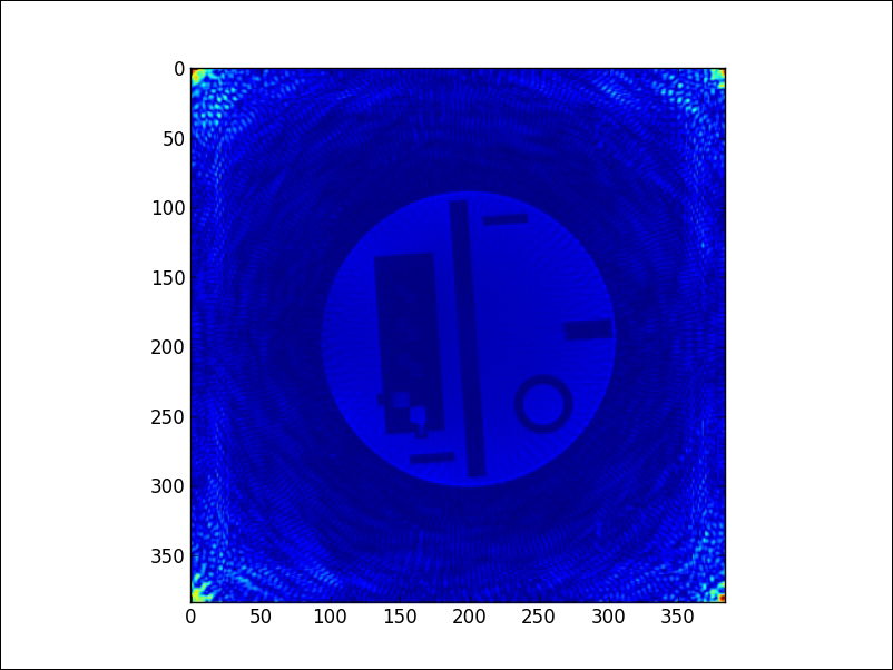
Those are six commented lines with information, one more line indicating the shape of the vector (63240 rows and 1 column), and the rest of the lines contain two columns of floating point values, the real and imaginary parts of the corresponding data. We proceed to read this vector to memory, solve the least squares problem suggested, and obtain the following reconstruction that represents a slice of the simulated human head:
In [12]: r_vals, i_vals = np.loadtxt("mri2_b.mtx", skiprows=7,
   ....:                             unpack=True)
In [13]: %time solution = spspla.lsqr(MRI2, r_vals + 1j*i_vals)
CPU times: user 4min 42s, sys: 1min 48s, total: 6min 30s
Wall time: 6min 30s
In [14]: from scipy.fftpack import fft2, fftshift
In [15]: img = solution[0].reshape(384,384); \
   ....: img = np.abs(fftshift(fft2(img)))
In [16]: plt.imshow(img); \
   ....: plt.show()
Tip
If interested in the theory behind the creation of this matrix and the particulars of this problem, read the article On the optimality of the Gridding Reconstruction Algorithm, by H. Sedarat and D. G. Nishimura, published in IEEE Trans. Medical Imaging, vol. 19, no. 4, pp. 306-317, 2000.
For matrices with a good structure, which are going to be exclusively involved in matrix multiplications, it is often possible to store the objects in smart ways. Let's consider an example.
A horizontal earthquake oscillation affects each floor of a tall building, depending on the natural frequencies of the oscillation of the floors. If we make certain assumptions, a model to quantize the oscillations on buildings with N floors can be obtained as a second-order system of N differential equations by competition: Newton's second law of force is set equal to the sum of Hooke's law of force, and the external force due to the earthquake wave.
These are the assumptions we will need:
Each floor is considered a point of mass located at its center-of-mass. The floors have masses
m[1], m[2], ..., m[N].Each floor is restored to its equilibrium position by a linear restoring force (Hooke's
-k * elongation). The Hooke's constants for the floors arek[1], k[2], ..., k[N].The locations of masses representing the oscillation of the floors are
x[1], x[2], ..., x[N]. We assume all of them functions of time and that at equilibrium, they are all equal to zero.For simplicity of exposition, we are going to assume no friction: all the damping effects on the floors will be ignored.
The equations of a floor depend only on the neighboring floors.
Set M, the mass matrix, to be a diagonal matrix containing the floor masses on its diagonal. Set K, the Hooke's matrix, to be a tri-diagonal matrix with the following structure, for each row j, all the entries are zero except for the following ones:
Column
j-1, which we set to bek[j+1],Column
j, which we set to-k[j+1]-k[j+1], andColumn
j+1, which we set tok[j+2].
Set H to be a column vector containing the external force on each floor due to the earthquake, and X, the column vector containing the functions x[j].
We have then the system: M * X'' = K * X + H. The homogeneous part of this system is the product of the inverse of M with K, which we denote as A.
To solve the homogeneous linear second-order system, X'' = A * X, we define the variable Y to contain 2*N entries: all N functions x[j], followed by their derivatives x'[j]. Any solution of this second-order linear system has a corresponding solution on the first-order linear system Y' = C * Y, where C is a block matrix of size 2*N × 2*N. This matrix C is composed by a block of size N × N containing only zeros, followed horizontally by the identity (of size N × N), and below these two, the matrix A followed horizontally by another N × N block of zeros.
It is not necessary to store this matrix C into memory, or any of its factors or blocks. Instead, we will make use of its structure, and use a linear operator to represent it. Minimal data is then needed to generate this operator (only the values of the masses and the Hooke's coefficients), much less than any matrix representation of it.
Let us show a concrete example with six floors. We indicate first their masses and Hooke's constants, and then, proceed to construct a representation of A as a linear operator:
In [17]: m = np.array([56., 56., 56., 54., 54., 53.]); \
   ....: k = np.array([561., 562., 560., 541., 542., 530.])
In [18]: def Axv(v):
   ....:     global k, m
   ....:     w = v.copy()
   ....:     w[0] = (k[1]*v[1] - (k[0]+k[1])*v[0])/m[0]
   ....:     for j in range(1, len(v)-1):
   ....:         w[j] = k[j]*v[j-1] + k[j+1]*v[j+1] - \
   ....:                (k[j]+k[j+1])*v[j]
   ....:         w[j] /= m[j]
   ....:     w[-1] = k[-1]*(v[-2]-v[-1])/m[-1]
   ....:     return w
   ....:
In [19]: A = spspla.LinearOperator((6,6), matvec=Axv, matmat=Axv,
   ....:                           dtype=np.float64)
The construction of C is very simple now (much simpler than that of its matrix!):
In [20]: def Cxv(v):
   ....:     n = len(v)/2
   ....:     w = v.copy()
   ....:     w[:n] = v[n:]
   ....:     w[n:] = A * v[:n]
   ....:     return w
   ....:
In [21]: C = spspla.LinearOperator((12,12), matvec=Cxv, matmat=Cxv,
   ....:                           dtype=np.float64)
A solution of this homogeneous system comes in the form of an action of the exponential of C: Y(t) = expm(C*t)* Y(0), where expm() here denotes a matrix exponential function. In SciPy, this operation is performed with the routine expm_multiply in the module scipy.sparse.linalg.
For example, in our case, given the initial value containing the values x[1](0)=0, ..., x[N](0)=0, x'[1](0)=1, ..., x'[N](0)=1, if we require a solution Y(t) for values of t between 0 and 1 in steps of size 0.1, we could issue the following:
Tip
It has been reported in some installations that, in the next step, a matrix for C must be given instead of the actual linear operator (thus contradicting the manual). If this is the case in your system, simply change C in the next lines to its matrix representation.
In [22]: initial_condition = np.zeros(12); \
   ....: initial_condition[6:] = 1
In [23]: Y = spspla.exp_multiply(C, np.zeros(12), start=0,
   ....:                         stop=1, num=10)
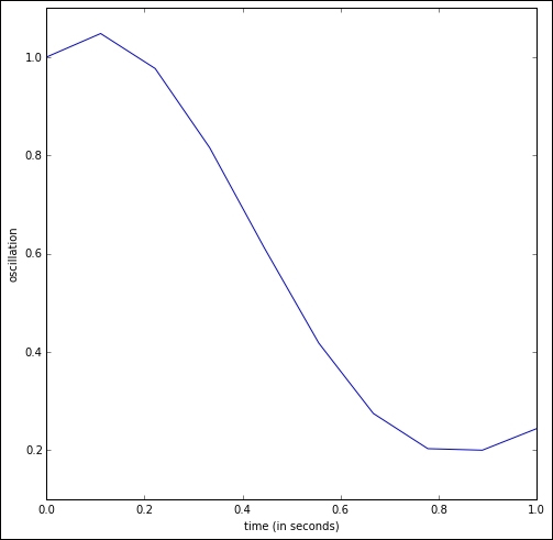
The oscillations of the six floors during the first second can then be calculated and plotted. For instance, to view the oscillation of the first floor, we could issue the following:
In [24]: plt.plot(np.linspace(0,1,10), Y[:,0]); \
   ....: plt.xlabel('time (in seconds)'); \
   ....: plt.ylabel('oscillation')
We obtain the following plot. Note how the first floor rises in the first tenth of a second, only to drop from 0.1 to 0.9 seconds from its original height to almost under a meter and then, start a slow rise:
Tip
For more details about systems of differential equations, and how to solve them with actions of exponentials, read, for example, the excellent book, Elementary Differential Equations 10 ed., by William E. Boyce and Richard C. DiPrima. Wiley, 2012.
These three examples illustrate the goal of this first chapter, Numerical Linear Algebra. In Python, this is accomplished first by storing the data in a matrix form, or as a related linear operator, by means of any of the following classes:
numpy.ndarray(making sure that they are two-dimensional)numpy.matrixscipy.sparse.bsr_matrix(Block Sparse Row matrix)scipy.sparse.coo_matrix(Sparse Matrix in COOrdinate format)scipy.sparse.csc_matrix(Compressed Sparse Column matrix)scipy.sparse.csr_matrix(Compressed Sparse Row matrix)scipy.sparse.dia_matrix(Sparse matrix with DIAgonal storage)scipy.sparse.dok_matrix(Sparse matrix based on a Dictionary of Keys)scipy.sparse.lil_matrix(Sparse matrix based on a linked list)scipy.sparse.linalg.LinearOperator
As we have seen in the examples, the choice of different classes obeys mainly to the sparsity of data and the algorithms that we are to apply to them.
This choice then dictates the modules that we use for the different algorithms: scipy.linalg for generic matrices and both scipy.sparse and scipy.sparse.linalg for sparse matrices or linear operators. These three SciPy modules are compiled on top of the highly optimized computer libraries BLAS (written in Fortran77), LAPACK (in Fortran90), ARPACK (in Fortran77), and SuperLU (in C).
Note
For a better understanding of these underlying packages, read the description and documentation from their creators:
BLAS: netlib.org/blas/faq.html
SuperLU: crd-legacy.lbl.gov/~xiaoye/SuperLU/
Most of the routines in these three SciPy modules are wrappers to functions in the mentioned libraries. If we so desire, we also have the possibility to call the underlying functions directly. In the scipy.linalg module, we have the following:
scipy.linalg.get_blas_funcsto call routines from BLASscipy.linalg.get_lapack_funcsto call routines from LAPACK
For example, if we want to use the BLAS function NRM2 to compute Frobenius norms:
In [25]: blas_norm = spla.get_blas_func('nrm2')
In [26]: blas_norm(np.float32([1e20]))
Out[26]: 1.0000000200408773e+20
In the first part of this chapter, we are going to focus on the effective creation of matrices. We start by recalling some different ways to construct a basic matrix as an ndarray instance class, including an enumeration of all the special matrices already included in NumPy and SciPy. We proceed to examine the possibilities of constructing complex matrices from basic ones. We review the same concepts within the matrix instance class. Next, we explore in detail the different ways to input sparse matrices. We finish the section with the construction of linear operators.
Note
We assume familiarity with ndarray creation in NumPy, as well as data types (dtype), indexing, routines for the combination of two or more arrays, array manipulation, or extracting information from these objects. In this chapter, we will focus on the functions, methods, and routines that are significant to matrices alone. We will disregard operations if their outputs have no translation into linear algebra equivalents. For a primer on ndarray, we recommend you to browse through Chapter 2, Top-Level SciPy of Learning SciPy for Numerical and Scientific Computing, Second Edition. For a quick review of Linear Algebra, we recommend Hoffman and Kunze, Linear Algebra 2nd Edition, Pearson, 1971.
We may create matrices from data as ndarray instances in three different ways: manually from standard input, by assigning to each entry a value from a function, or by retrieving the data from external files.
|
Constructor |
Description |
|---|---|
|
|
Create a matrix from |
|
|
Create diagonal matrix with entries of array |
|
|
Create a matrix by executing a function over each coordinate |
|
|
Create a matrix from a text or binary file (basic) |
|
|
Create a matrix from a text file (advanced) |
Let us create some example matrices to illustrate some of the functions defined in the previous table. As before, we start an iPython session:
In [1]: import numpy as np, matplotlib.pyplot as plt, \
   ...: scipy.linalg as spla, scipy.sparse as spsp, \
   ...: scipy.sparse.linalg as spspla
In [2]: A = np.array([[1,2],[4,16]]); \...: A
Out[2]:
array([[ 1,  2],
       [ 4, 16]])
In [3]: B = np.fromfunction(lambda i,j: (i-1)*(j+1),
   ...:                     (3,2), dtype=int); \
   ...: print B
   ...:
 [[-1 -2]
  [ 0  0]
  [ 1  2]]
In [4]: np.diag((1j,4))
Out[4]:
array([[ 0.+1.j,  0.+0.j],
       [ 0.+0.j,  4.+0.j]])
Special matrices with predetermined zeros and ones can be constructed with the following functions:
|
Constructor |
Description |
|---|---|
|
|
Array of a given shape, entries not initialized |
|
|
2-D array with ones on the k-th diagonal, and zeros elsewhere |
|
|
Identity array |
|
|
Array with all entries equal to one |
|
|
Array with all entries equal to zero |
|
|
Array with ones at and below the given diagonal, zeros otherwise |
Tip
All these constructions, except numpy.tri, have a companion function xxx_like that creates ndarray with the requested characteristics and with the same shape and data type as another source ndarray class:
In [5]: np.empty_like(A)
Out[5]:
array([[140567774850560, 140567774850560],
       [     4411734640, 562954363882576]])
Of notable importance are arrays constructed as numerical ranges.
|
Constructor |
Description |
|---|---|
|
|
Evenly spaced values within an interval |
|
|
Evenly spaced numbers over an interval |
|
|
Evenly spaced numbers on a log scale |
|
|
Coordinate matrices from two or more coordinate vectors |
|
|
|
|
|
|
Special matrices with numerous applications in linear algebra can be easily called from within NumPy and the module scipy.linalg.
|
Constructor |
Description |
|---|---|
|
|
Circulant matrix generated by 1-D array |
|
|
Companion matrix of polynomial with coefficients coded by |
|
|
Sylvester's construction of a Hadamard matrix of size n × n. n must be a power of 2 |
|
|
Hankel matrix with |
|
|
Hilbert matrix of size n × n |
|
|
The inverse of a Hilbert matrix of size n × n |
|
|
Leslie matrix with fecundity array |
|
|
n × n truncations of the Pascal matrix of binomial coefficients |
|
|
Toeplitz array with first column |
|
|
Van der Monde matrix of array |
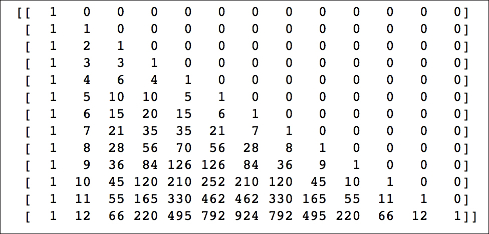
For instance, one fast way to obtain all binomial coefficients of orders up to a large number (the corresponding Pascal triangle) is by means of a precise Pascal matrix. The following example shows how to compute these coefficients up to order 13:
In [6]: print spla.pascal(13, kind='lower')
Besides these basic constructors, we can always stack arrays in different ways:
|
Constructor |
Description |
|---|---|
|
|
Join matrices together |
|
|
Stack matrices horizontally |
|
|
Stack matrices vertically |
|
|
Repeat a matrix a certain number of times (given by |
|
|
Create a block diagonal array |
Let us observe some of these constructors in action:
In [7]: np.tile(A, (2,3))   # 2 rows, 3 columns
Out[7]:
array([[ 1,  2,  1,  2,  1,  2],
       [ 4, 16,  4, 16,  4, 16],
       [ 1,  2,  1,  2,  1,  2],
       [ 4, 16,  4, 16,  4, 16]])
In [8]: spla.block_diag(A,B)
Out[8]:
array([[ 1,  2,  0,  0],
       [ 4, 16,  0,  0],
       [ 0,  0, -1, -2],
       [ 0,  0,  0,  0],
       [ 0,  0,  1,  2]])
For the matrix class, the usual way to create a matrix directly is to invoke either numpy.mat or numpy.matrix. Observe how much more comfortable is the syntax of numpy.matrix than that of numpy.array, in the creation of a matrix similar to A. With this syntax, different values separated by commas belong to the same row of the matrix. A semi-colon indicates a change of row. Notice the casting to the matrix class too!
In [9]: C = np.matrix('1,2;4,16'); \
   ...: C
Out[9]:
matrix([[ 1,  2],
        [ 4, 16]])
These two functions also transform any ndarray into matrix. There is a third function that accomplishes this task: numpy.asmatrix:
In [10]: np.asmatrix(A)
Out[10]:
matrix([[ 1,  2],
        [ 4, 16]])
For arrangements of matrices composed by blocks, besides the common stack operations for ndarray described before, we have the extremely convenient function numpy.bmat. Note the similarity with the syntax of numpy.matrix, particularly the use of commas to signify horizontal concatenation and semi-colons to signify vertical concatenation:
In [11]: np.bmat('A;B')        In [12]: np.bmat('A,C;C,A')
Out[11]:                       Out[12]:
matrix([[ 1,  2],              matrix([[ 1,  2,  1,  2],
        [ 4, 16],                      [ 4, 16,  4, 16],
        [-1, -2],                      [ 1,  2,  1,  2],
        [ 0,  0],                      [ 4, 16,  4, 16]])
        [ 1,  2]])
There are seven different ways to input sparse matrices. Each format is designed to make a specific problem or operation more efficient. Let us go over them in detail:
They can be populated in up to five ways, three of which are common to every sparse matrix format:
They can cast to sparse any generic matrix. The
lilformat is the most effective with this method:In [13]: A_coo = spsp.coo_matrix(A); \ ....: A_lil = spsp.lil_matrix(A)
They can cast to a specific sparse format another sparse matrix in another sparse format:
In [14]: A_csr = spsp.csr_matrix(A_coo)Empty sparse matrices of any shape can be constructed by indicating the shape and
dtype:In [15]: M_bsr = spsp.bsr_matrix((100,100), dtype=int)
They all have several different extra input methods, each specific to their storage format.
Fancy indexing: As we would do with any generic matrix. This is only possible with the LIL or DOK formats:
In [16]: M_lil = spsp.lil_matrix((100,100), dtype=int)
In [17]: M_lil[25:75, 25:75] = 1
In [18]: M_bsr[25:75, 25:75] = 1
NotImplementedError    Traceback (most recent call last)
<ipython-input-18-d9fa1001cab8> in <module>()
----> 1 M_bsr[25:75, 25:75] = 1
[...]/scipy/sparse/bsr.pyc in __setitem__(self, key, val)
    297
    298     def __setitem__(self,key,val):
--> 299         raise NotImplementedError
    300
    301     ######################
NotImplementedError:
Dictionary of keys: This input system is most effective when we create, update, or search each element one at a time. It is efficient only for the LIL and DOK formats:
In [19]: M_dok = spsp.dok_matrix((100,100), dtype=int)
In [20]: position = lambda i, j: ((i<j) & ((i+j)%10==0))
In [21]: for i in range(100):
   ....:     for j in range(100):
   ....:         M_dok[i,j] = position(i,j)
   ....:
Data, rows, and columns: This is common to four formats: BSR, COO, CSC, and CSR. This is the method of choice to import sparse matrices from the Matrix Market Exchange format, as illustrated at the beginning of the chapter.
Tip
With the data, rows, and columns input method, it is a good idea to always include the option
shapein the construction. In case this is not provided, the size of the matrix will be inferred from the largest coordinates from the rows and columns, resulting possibly in a matrix of a smaller size than required.Data, indices, and pointers: This is common to three formats: BSR, CSC, and CSR. It is the method of choice to import sparse matrices from the Rutherford-Boeing Exchange format.
Note
The Rutherford-Boeing Exchange format is an updated version of the Harwell-Boeing format. It stores the matrix as three vectors:
pointers_v,indices_v, anddata. The row indices of the entries of the jth column are located in positionspointers_v(j)throughpointers_v(j+1)-1of the vectorindices_v. The corresponding values of the matrix are located at the same positions, in the vector data.
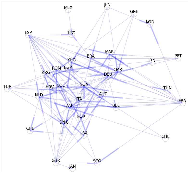
Let us show by example how to read an interesting matrix in the Rutherford-Boeing matrix exchange format, Pajek/football. This 35 × 35 matrix with 118 non-zero entries can be found in the collection at www.cise.ufl.edu/research/sparse/matrices/Pajek/football.html.
It is an adjacency matrix for a network of all the national football teams that attended the FIFA World Cup celebrated in France in 1998. Each node in the network represents one country (or national football team) and the links show which country exported players to another country.
This is a printout of the football.rb file:
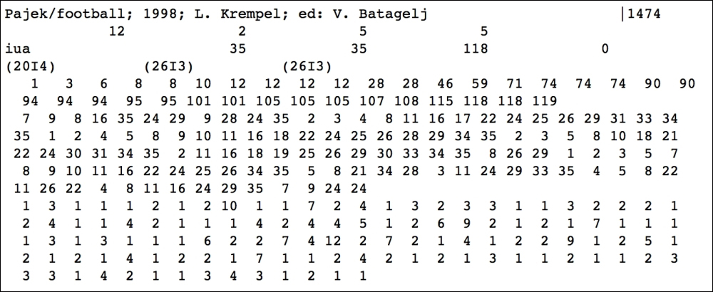
The header of the file (the first four lines) contains important information:
The first line provides us with the title of the matrix,
Pajek/football; 1998; L. Krempel; ed: V. Batagelj, and a numerical key for identification purposesMTRXID=1474.The second line contains four integer values:
TOTCRD=12(lines containing significant data after the header; see In [24]),PTRCRD=2(number of lines containing pointer data),INDCRD=5(number of lines containing indices data), andVALCRD=2(number of lines containing the non-zero values of the matrix). Note that it must be TOTCRD = PTRCRD + INDCRD + VALCRD.The third line indicates the matrix type
MXTYPE=(iua), which in this case stands for an integer matrix, unsymmetrical, compressed column form. It also indicates the number of rows and columns (NROW=35,NCOL=35), and the number of non-zero entries (NNZERO=118). The last entry is not used in the case of a compressed column form, and it is usually set to zero.The fourth column contains the Fortran formats for the data in the following columns.
PTRFMT=(20I4)for the pointers,INDFMT=(26I3)for the indices, andVALFMT=(26I3)for the non-zero values.
We proceed to opening the file for reading, storing each line after the header in a Python list, and extracting from the relevant lines of the file, the data we require to populate the vectors indptr, indices, and data. We finish by creating the corresponding sparse matrix called football in the CSR format, with the data, indices, pointers method:
In [22]: f = open("football.rb", 'r'); \
   ....: football_list = list(f); \
   ....: f.close()
In [23]: football_data = np.array([])
In [24]: for line in range(4, 4+12):
   ....:     newdata = np.fromstring(football_list[line], sep=" ")
   ....:     football_data = np.append(football_data, newdata)
   ....:
In [25]: indptr = football_data[:35+1] - 1; \
   ....: indices = football_data[35+1:35+1+118] - 1; \
   ....: data = football_data[35+1+118:]
In [26]: football = spsp.csr_matrix((data, indices, indptr),
   ....:                            shape=(35,35))
At this point, it is possible to visualize the network with its associated graph, with the help of a Python module called networkx. We obtain the following diagram depicting as nodes the different countries. Each arrow between the nodes indicates the fact that the originating country has exported players to the receiving country:
Note
networkx is a Python module to deal with complex networks. For more information, visit their Github project pages at networkx.github.io.
One way to accomplish this task is as follows:
In [27]: import networkx
In [28]: G = networkx.DiGraph(football)
In [29]: f = open("football_nodename.txt"); \
   ....: m = list(f); \
   ....: f.close()
In [30]: def rename(x): return m[x]
In [31]: G = networkx.relabel_nodes(G, rename)
In [32]: pos = networkx.spring_layout(G)
In [33]: networkx.draw_networkx(G, pos, alpha=0.2, node_color='w',
   ....:                        edge_color='b')
The module scipy.sparse borrows from NumPy some interesting concepts to create constructors and special matrices:
|
Constructor |
Description |
|---|---|
|
|
Sparse matrix from diagonals |
|
|
Random sparse matrix of prescribed density |
|
|
Sparse matrix with ones in the main diagonal |
|
|
Identity sparse matrix of size n × n |
Both functions diags and rand deserve examples to show their syntax. We will start with a sparse matrix of size 14 × 14 with two diagonals: the main diagonal contains 1s, and the diagonal below contains 2s. We also create a random matrix with the function scipy.sparse.rand. This matrix has size 5 × 5, with 25 percent non-zero elements (density=0.25), and is crafted in the LIL format:
In [34]: diagonals = [[1]*14, [2]*13]
In [35]: print spsp.diags(diagonals, [0,-1]).todense()
[[ 1.  0.  0.  0.  0.  0.  0.  0.  0.  0.  0.  0.  0.  0.]
 [ 2.  1.  0.  0.  0.  0.  0.  0.  0.  0.  0.  0.  0.  0.]
 [ 0.  2.  1.  0.  0.  0.  0.  0.  0.  0.  0.  0.  0.  0.]
 [ 0.  0.  2.  1.  0.  0.  0.  0.  0.  0.  0.  0.  0.  0.]
 [ 0.  0.  0.  2.  1.  0.  0.  0.  0.  0.  0.  0.  0.  0.]
 [ 0.  0.  0.  0.  2.  1.  0.  0.  0.  0.  0.  0.  0.  0.]
 [ 0.  0.  0.  0.  0.  2.  1.  0.  0.  0.  0.  0.  0.  0.]
 [ 0.  0.  0.  0.  0.  0.  2.  1.  0.  0.  0.  0.  0.  0.]
 [ 0.  0.  0.  0.  0.  0.  0.  2.  1.  0.  0.  0.  0.  0.]
 [ 0.  0.  0.  0.  0.  0.  0.  0.  2.  1.  0.  0.  0.  0.]
 [ 0.  0.  0.  0.  0.  0.  0.  0.  0.  2.  1.  0.  0.  0.]
 [ 0.  0.  0.  0.  0.  0.  0.  0.  0.  0.  2.  1.  0.  0.]
 [ 0.  0.  0.  0.  0.  0.  0.  0.  0.  0.  0.  2.  1.  0.]
 [ 0.  0.  0.  0.  0.  0.  0.  0.  0.  0.  0.  0.  2.  1.]]
In [36]: S_25_lil = spsp.rand(5, 5, density=0.25, format='lil')
In [37]: S_25_lil
Out[37]:
<5x5 sparse matrix of type '<type 'numpy.float64'>'
        with 6 stored elements in LInked List format>
In [38]: print S_25_lil
  (0, 0)    0.186663044982
  (1, 0)    0.127636181284
  (1, 4)    0.918284870518
  (3, 2)    0.458768884701
  (3, 3)    0.533573291684
  (4, 3)    0.908751420065
In [39]: print S_25_lil.todense()
[[ 0.18666304  0.          0.          0.          0.        ]
 [ 0.12763618  0.          0.          0.          0.91828487]
 [ 0.          0.          0.          0.          0.        ]
 [ 0.          0.          0.45876888  0.53357329  0.        ]
 [ 0.          0.          0.          0.90875142  0.        ]]
Similar to the way we combined ndarray instances, we have some clever ways to combine sparse matrices to construct more complex objects:
|
Constructor |
Description |
|---|---|
|
|
Sparse matrix from sparse sub-blocks |
|
|
Stack sparse matrices horizontally |
|
|
Stack sparse matrices vertically |
A linear operator is basically a function that takes as input a column vector and outputs another column vector, by left multiplication of the input with a matrix. Although technically, we could represent these objects just by handling the corresponding matrix, there are better ways to do this.
|
Constructor |
Description |
|---|---|
|
|
Common interface for performing matrix vector products |
|
|
Return |
In the scipy.sparse.linalg module, we have a common interface that handles these objects: the LinearOperator class. This class has only the following two attributes and three methods:
shape: The shape of the representing matrixdtype: The data type of the matrixmatvec: To perform multiplication of a matrix with a vectorrmatvec: To perform multiplication by the conjugate transpose of a matrix with a vectormatmat: To perform multiplication of a matrix with another matrix
Its usage is best explained through an example. Consider two functions that take vectors of size 3, and output vectors of size 4, by left multiplication with two respective matrices of size 4 × 3. We could very well define these functions with lambda predicates:
In [40]: H1 = np.matrix("1,3,5; 2,4,6; 6,4,2; 5,3,1"); \
   ....: H2 = np.matrix("1,2,3; 1,3,2; 2,1,3; 2,3,1")
In [41]: L1 = lambda x: H1.dot(x); \
   ....: L2 = lambda x: H2.dot(x)
In [42]: print L1(np.ones(3))
[[  9.  12.  12.   9.]]
In [43]: print L2(np.tri(3,3))
 [[ 6.  5.  3.]
  [ 6.  5.  2.]
  [ 6.  4.  3.]
  [ 6.  4.  1.]]
Now, one issue arises when we try to add/subtract these two functions, or multiply any of them by a scalar. Technically, it should be as easy as adding/subtracting the corresponding matrices, or multiplying them by any number, and then performing the required left multiplication again. But that is not the case.
For instance, we would like to write (L1+L2)(v) instead of L1(v) + L2(v). Unfortunately, doing so will raise an error:
TypeError: unsupported operand type(s) for +: 'function' and
'function'
Instead, we may instantiate the corresponding linear operators and manipulate them at will, as follows:
In [44]: Lo1 = spspla.aslinearoperator(H1); \
   ....: Lo2 = spspla.aslinearoperator(H2)
In [45]: Lo1 - 6 * Lo2
Out[45]: <4x3 _SumLinearOperator with dtype=float64>
In [46]: print Lo1 * np.ones(3)
[  9.  12.  12.  9.]
In [47]: print (Lo1-6*Lo2) * np.tri(3,3)
[[-27. -22. -13.]
 [-24. -20.  -6.]
 [-24. -18. -16.]
 [-27. -20.  -5.]]
Linear operators are a great advantage when the amount of information needed to describe the product with the related matrix is less than the amount of memory needed to store the non-zero elements of the matrix.
For instance, a permutation matrix is a square binary matrix (ones and zeros) that has exactly one entry in each row and each column. Consider a large permutation matrix, say 1024 × 1024, formed by four blocks of size 512 × 512: a zero block followed horizontally by an identity block, on top of an identity block followed horizontally by another zero block. We may store this matrix in three different ways:
In [47]: P_sparse = spsp.diags([[1]*512, [1]*512], [512,-512], \
   ....:                       dtype=int)
In [48]: P_dense = P_sparse.todense()
In [49]: mv = lambda v: np.roll(v, len(v)/2)
In [50]: P_lo = spspla.LinearOperator((1024,1024), matvec=mv, \
   ....:                              matmat=mv, dtype=int)
In the sparse case, P_sparse, we may think of this as the storage of just 1024 integer numbers. In the dense case, P_dense, we are technically storing 1048576 integer values. In the case of the linear operator, it actually looks like we are not storing anything! The function mv that indicates how to perform the multiplications has a much smaller footprint than any of the related matrices. This is also reflected in the time of execution of the multiplications with these objects:
In [51]: %timeit P_sparse * np.ones(1024)
10000 loops, best of 3: 29.7 µs per loop
In [52]: %timeit P_dense.dot(np.ones(1024))
100 loops, best of 3: 6.07 ms per loop
In [53]: %timeit P_lo * np.ones(1024)
10000 loops, best of 3: 25.4 µs per loop
The emphasis of the second part of this chapter is on mastering the following operations:
Scalar multiplication, matrix addition, and matrix multiplication
Traces and determinants
Transposes and inverses
Norms and condition numbers
Let us start with the matrices stored with the ndarray class. We accomplish scalar multiplication with the * operator, and the matrix addition with the + operator. But for matrix multiplication we will need the instance method dot() or the numpy.dot function, since the operator * is reserved for element-wise multiplication:
In [54]: 2*A
Out[54]:
array([[ 2,  4],
       [ 8, 32]])
In [55]: A + 2*A
Out[55]:
array([[ 3,  6],
       [12, 48]])
In [56]: A.dot(2*A)       In [56]: np.dot(A, 2*A)
Out[56]:                  Out[56]:
array([[ 18,  68],        array([[ 18,  68],
       [136, 528]])              [136, 528]])
In [57]: A.dot(B)
ValueError: objects are not aligned
In [58]: B.dot(A)         In [58]: np.dot(B, A)
Out[58]:                  Out[58]:
array([[ -9, -34],        array([[ -9, -34],
       [  0,   0],               [  0,   0],
       [  9,  34]])              [  9,  34]])
The matrix class makes matrix multiplication more intuitive: the operator * can be used instead of the dot() method. Note also how matrix multiplication between different instance classes ndarray and a matrix is always casted to a matrix instance class:
In [59]: C * B
ValueError: shapes (2,2) and (3,2) not aligned: 2 (dim 1) != 3 (dim 0)
In [60]: B * C
Out[60]:
matrix([[ -9, -34],
        [  0,   0],
        [  9,  34]])
For sparse matrices, both scalar multiplication and addition work well with the obvious operators, even if the two sparse classes are not the same. Note the resulting class casting after each operation:
In [61]: S_10_coo = spsp.rand(5, 5, density=0.1, format='coo')
In [62]: S_25_lil + S_10_coo
Out[62]: <5x5 sparse matrix of type '<type 'numpy.float64'>'
        with 8 stored elements in Compressed Sparse Row format>
In [63]: S_25_lil * S_10_coo
Out[63]: <5x5 sparse matrix of type '<type 'numpy.float64'>'
        with 4 stored elements in Compressed Sparse Row format>
Tip
numpy.dot does not work well for matrix multiplication of a sparse matrix with a generic. We must use the operator * instead.
In [64]: S_100_coo = spsp.rand(2, 2, density=1, format='coo')
In [65]: np.dot(A, S_100_coo)
Out[66]:
array([[ <2x2 sparse matrix of type '<type 'numpy.float64'>'
  with 4 stored elements in COOrdinate format>,
        <2x2 sparse matrix of type '<type 'numpy.float64'>'
  with 4 stored elements in COOrdinate format>],
       [ <2x2 sparse matrix of type '<type 'numpy.float64'>'
  with 4 stored elements in COOrdinate format>,
        <2x2 sparse matrix of type '<type 'numpy.float64'>'
  with 4 stored elements in COOrdinate format>]], dtype=object)
In [67]: A * S_100_coo
Out[68]:
array([[  1.81 ,   1.555],
       [ 11.438,  11.105]])
The traces of a matrix are the sums of the elements on the diagonals (assuming always increasing indices in both dimensions). For generic matrices, we compute them with the instance method trace(), or with the function numpy.trace:
In [69]: A.trace()        In [71]: C.trace()
Out[69]: 17               Out[71]: matrix([[17]])
In [70]: B.trace()        In [72]: np.trace(B, offset=-1)
Out[70]: -1               Out[72]: 2
In order to compute the determinant of generic square matrices, we need the function det in the module scipy.linalg:
In [73]: spla.det(C)
Out[73]: 8.0
Transposes can be computed with any of the two instance methods transpose() or T, for any of the two classes of generic matrices:
In [74]: B.transpose()        In [75]: C.T
Out[74]:                      Out[75]:
array([[-1,  0,  1],          matrix([[ 1,  4],
       [-2,  0,  2]])                 [ 2, 16]])
Hermitian transpose can be computed for the matrix class with the instance method H:
In [76]: D = C * np.diag((1j,4)); print D     In [77]: print D.H
[[  0.+1.j   8.+0.j]                          [[  0.-1.j   0.-4.j]
 [  0.+4.j  64.+0.j]]                          [  8.-0.j  64.-0.j]]
Inverses of non-singular square matrices are computed for the ndarray class with the function inv in the module scipy.linalg. For the matrix class, we may also use the instance method I. For non-singular square sparse matrices, we may use the function inv in the module scipy.sparse.linalg.
Tip
Inverses of sparse matrices are seldom sparse. For this reason, it is not recommended to perform this operation with the scipy.sparse.inv function. One possible way to go around this issue is to convert the matrix to generic with the todense() instance method, and use scipy.linear.inv instead.
But due to the difficulty of inverting large matrices, it is often beneficial to compute approximations to the inverse, instead. The function spilu in the module scipy.sparse.linalg provides us with a very fast algorithm to perform this computation for square sparse matrices in CSC format. This algorithm is based on LU decompositions, and coded internally as a wrapper of a function from the library SuperLU. Its use is rather complex, and we are going to postpone its study until we explore matrix factorizations.
In [78]: E = spsp.rand(512, 512, density=1).todense()
In [79]: S_100_csc = spsp.rand(512, 512, density=1, format='csc')
In [80]: %timeit E.I
10 loops, best of 3: 28.7 ms per loop
In [81]: %timeit spspla.inv(S_100_csc)
1 loops, best of 3: 1.99 s per loop
Note
In the execution of sparse inverses, if the input matrix is not in the CSC or CSR format, we will get a warning:
/scipy/sparse/linalg/dsolve/linsolve.py:88: SparseEfficiencyWarning: spsolve requires A be CSC or CSR matrix format
  warn('spsolve requires A be CSC or CSR matrix format', SparseEfficiencyWarning)
/scipy/sparse/linalg/dsolve/linsolve.py:103: SparseEfficiencyWarning: solve requires b be CSC or CSR matrix format
The Moore-Penrose pseudo-inverse can be computed for any kind of matrix (not necessarily square) with either routines the pinv or the pinv2 in the module scipy.linalg. The first method, pinv, resorts to solving a least squares problem to compute the pseudo-inverse. The function pinv2 computes the pseudo-inverse by a method based on singular value decompositions. For Hermitian matrices, or matrices that are symmetric with no complex coefficients, we also have a third function called pinvh, which is based on eigenvalue decompositions.
It is known that in the case of square non-singular matrices, the inverse and pseudo-inverse are the same. This simple example shows the times of computation of the inverses of a large generic symmetric matrix with the five methods described:
In [82]: F = E + E.T     # F is symmetric
In [83]: %timeit F.I
1 loops, best of 3: 24 ms per loop
In [84]: %timeit spla.inv(F)
10 loops, best of 3: 28 ms per loop
In [85]: %timeit spla.pinvh(E)
1 loops, best of 3: 120 ms per loop
In [86]: %timeit spla.pinv2(E)
1 loops, best of 3: 252 ms per loop
In [87]: %timeit spla.pinv(F)
1 loops, best of 3: 2.21 s per loop
For generic matrices, we have seven different standard norms in scipy.linalg. We can summarize them in the following table:
|
Constructor |
Description |
|---|---|
|
|
Sum of absolute values of entries in each row. Pick the largest value. |
|
|
Sum of absolute values of entries in each row. Pick the smallest value. |
|
|
Sum of absolute values of entries in each column. Pick the largest value. |
|
|
Sum of absolute values of entries in each column. Pick the smallest value. |
|
|
Largest eigenvalue of the matrix. |
|
|
Smallest eigenvalue of the matrix. |
|
|
Frobenius norm: the square root of the trace of the product A.H * A. |
In [88]: [spla.norm(A,s) for s in (np.inf,-np.inf,-1,1,-2,2,'fro')]
Out[88]: [20, 3, 5, 18, 0.48087417361008861, 16.636368595013604, 16.643316977093239]
Tip
For sparse matrices, we can always compute norms by applying the todense() instance method prior to computation. But when the sizes of the matrices are too large, this is very impractical. In those cases, the best we can get for the 1-norm is a lower bound, thanks to the function onenormest in the module scipy.sparse.linalg:
In [89]: spla.norm(S_100_csc.todense(), 1) - \
   ....: spspla.onenormest(S_100_csc)
Out[89]: 0.0
As for the 2-norms, we may find the values of the smallest and the largest eigenvalue, but only for square matrices. We have two algorithms in the module scipy.sparse.linalg that perform this task: eigs (for generic square matrices) and eigsh for real symmetric matrices. We will explore them in detail when we discuss matrix decompositions and factorizations in the next section.
Note the subtle difference between the norm computations from SciPy and NumPy. For example, in the case of the Frobenius norm, scipy.linalg.norm is based directly on the BLAS function called NRM2, while numpy.linalg.norm is equivalent to a purely straightforward computation of the form sqrt(add.reduce((x.conj() * x).real)). The advantage of the code based on BLAS, besides being much faster, is clear when some of the data is too large or too small in single-precision arithmetic. This is shown in the following example:
In [89]: a = np.float64([1e20]); \
   ....: b = np.float32([1e20])
In [90]: [np.linalg.norm(a), spla.norm(a)]
Out[90]: [1e+20, 1e+20]
In [91]: np.linalg.norm(b)
[...]/numpy/linalg/linalg.py:2056: RuntimeWarning: overflow encountered in multiply
  return sqrt(add.reduce((x.conj() * x).real, axis=None))
Out[91]: inf
In [92]: spla.norm(b)
Out[92]: 1.0000000200408773e+20
This brings us inevitably to a discussion about the computation of the condition number of a non-singular square matrix A. This value measures how much the output of the solution to the linear equation A * x = b will change when we make small changes to the input argument b. If this value is close to one, we can rest assured that the solution is going to change very little (we say then that the system is well-conditioned). If the condition number is large, we know that there might be issues with the computed solutions of the system (and we say then that it is ill-conditioned).
The computation of this condition number is performed by multiplying the norm of A with the norm of its inverse. Note that there are different condition numbers, depending on the norm that we choose for the computation. These values can also be computed for each of the pre-defined norms with the function numpy.linalg.cond, although we need to be aware of its obvious limitations.
In [93]: np.linalg.cond(C, -np.inf)
Out[93]: 1.875
A matrix function is a function that maps a square matrix to another square matrix via a power series. These should not be confused with vectorization: the application of any given function of one variable to each element of a matrix. For example, it is not the same to compute the square of a square matrix, A.dot(A) (for example, In [8]), than a matrix with all the elements of A squared (examples In [5] through In []).
Note
To make the proper distinction in notation, we will write A^2 to denote the actual square of a square matrix and A^n to represent the subsequent powers (for all positive integers n).
|
Constructor |
Description |
|---|---|
|
|
Extension of a scalar-valued function called |
|
|
Fractional matrix power |
|
|
Matrix exponential |
|
|
Action of the matrix exponential of |
|
|
Frechet derivative of the matrix exponential in the |
|
|
Matrix cosine |
|
|
Matrix sine |
|
|
Matrix tangent |
|
|
Hyperbolic matrix cosine |
|
|
Hyperbolic matrix sine |
|
|
Hyperbolic matrix tangent |
|
|
Matrix sign function |
|
|
Matrix square root |
|
|
Matrix logarithm |
In [1]: import numpy as np, scipy as sp; \
   ...: import scipy.linalg as spla
In [2]: np.set_printoptions(suppress=True, precision=3)
In [3]: def square(x): return x**2
In [4]: A = spla.hilbert(4); print A
[[ 1.     0.5    0.333  0.25 ]
 [ 0.5    0.333  0.25   0.2  ]
 [ 0.333  0.25   0.2    0.167]
 [ 0.25   0.2    0.167  0.143]]
In [5]: print square(A)
[[ 1.     0.25   0.111  0.062]
 [ 0.5    0.333  0.25   0.2  ]
 [ 0.333  0.25   0.2    0.167]
 [ 0.25   0.2    0.167  0.143]]
In [6]: print A*A
[[ 1.     0.25   0.111  0.062]
 [ 0.25   0.111  0.062  0.04 ]
 [ 0.111  0.062  0.04   0.028]
 [ 0.062  0.04   0.028  0.02 ]]
In [7]: print A**2
[[ 1.     0.25   0.111  0.062]
 [ 0.25   0.111  0.062  0.04 ]
 [ 0.111  0.062  0.04   0.028]
 [ 0.062  0.04   0.028  0.02 ]]
In [8]: print A.dot(A)
[[ 1.424  0.8    0.567  0.441]
 [ 0.8    0.464  0.333  0.262]
 [ 0.567  0.333  0.241  0.19 ]
 [ 0.441  0.262  0.19   0.151]]
The actual powers A^n of a matrix is the starting point for the definition of any matrix function. In the module numpy.linalg we have the routine matrix_power to perform this operation. We can also achieve this result with the generic function funm or with the function fractional_matrix_power, both of them in the module scipy.linalg.
In [9]: print np.linalg.matrix_power(A, 2)
[[ 1.424  0.8    0.567  0.441]
 [ 0.8    0.464  0.333  0.262]
 [ 0.567  0.333  0.241  0.19 ]
 [ 0.441  0.262  0.19   0.151]]
In [10]: print spla.fractional_matrix_power(A, 2)
[[ 1.424  0.8    0.567  0.441]
 [ 0.8    0.464  0.333  0.262]
 [ 0.567  0.333  0.241  0.19 ]
 [ 0.441  0.262  0.19   0.151]]
In [11]: print spla.funm(A, square)
[[ 1.424  0.8    0.567  0.441]
 [ 0.8    0.464  0.333  0.262]
 [ 0.567  0.333  0.241  0.19 ]
 [ 0.441  0.262  0.19   0.151]]
To compute any matrix function, theoretically, we first express the function as a power series, by means of its Taylor expansion. Then, we apply the input matrix into an approximation to that expansion (since it is impossible to add matrices ad infinitum). Most matrix functions necessarily carry an error of computation, for this reason. In the scipy.linalg module, the matrix functions are coded following this principle.
Note that there are three functions with an optional Boolean parameter
disp. To understand the usage of this parameter, we must remember that most matrix functions compute approximations, with an error of computation. The parameterdispis set toTrueby default, and it produces a warning if the error of approximation is large. If we setdisptoFalse, instead of a warning we will obtain the 1-norm of the estimated error.The algorithms behind the functions
expm, the action of an exponential over a matrix,expm_multiply, and the Frechet derivative of an exponential,expm_frechet, use Pade approximations instead of Taylor expansions. This allows for more robust and accurate calculations. All the trigonometric and hyperbolic trigonometric functions base their algorithm in easy computations involvingexpm.The generic matrix function called
funmand the square-root function calledsqrtmapply clever algorithms that play with the Schur decomposition of the input matrix, and proper algebraic manipulations with the corresponding eigenvalues. They are still prone to roundoff errors but are much faster and more accurate than any algorithm based on Taylor expansions.The matrix sign function called
signmis initially an application offunmwith the appropriate function, but should this approach fail, the algorithm takes a different approach based on iterations that converges to a decent approximation to the solution.The functions
logmandfractional_matrix_power(when the latter is applied to non-integer powers) use a very complex combination (and improvement!) of Pade approximations and Schur decompositions.
Tip
We will explore Schur decompositions when we deal with matrix factorizations related to eigenvalues. In the meantime, if you are interested in learning the particulars of these clever algorithms, read their descriptions in Golub and Van Loan, Matrix Computations 4 edition, Johns Hopkins Studies in the Mathematical Sciences, vol. 3.
For details on the improvements to Schur-Pade algorithms, as well as the algorithm behind Frechet derivatives of the exponential, refer to:
Nicholas J. Higham and Lijing Lin An Improved Schur-Pade Algorithm for Fractional Powers of a Matrix and Their Frechet Derivatives
Awad H. Al-Mohy and Nicholas J. Higham Improved Inverse Scaling and Squaring Algorithms for the Matrix Logarithm, in SIAM Journal on Scientific Computing, 34 (4)
The concept of matrix decompositions is what makes Numerical Linear Algebra an efficient tool in Scientific Computing. If the matrix representing a problem is simple enough, any basic generic algorithm can find the solutions optimally (that is, fast, with minimal storage of data, and without a significant roundoff error). But, in real life, this situation seldom occurs. What we do in the general case is finding a suitable matrix factorization and tailoring an algorithm that is optimal on each factor, thus gaining on each step an obvious advantage. In this section, we explore the different factorizations included in the modules scipy.linalg and scipy.sparse.linalg that help us achieve a robust solution to matrix equations.
We have the following factorizations in this category:
It is always possible to perform a factorization of a square matrix A as a product A = P ● L ● U of a permutation matrix P (which performs a permutation of the rows of A), a lower triangular matrix L, and an upper triangular matrix U:
|
Constructor |
Description |
|---|---|
|
|
Pivoted LU decomposition |
|
|
Pivoted LU decomposition |
|
|
Pivoted LU decomposition |
|
|
Incomplete pivoted LU decomposition |
For a square, symmetric, and positive definite matrix A, we can realize the matrix as the product A = UT ● U of an upper triangular matrix U with its transpose, or as the product A = LT ● L of a lower triangular matrix L with its transpose. All the diagonal entries of U or L are strictly positive numbers:
|
Constructor |
Description |
|---|---|
|
|
Cholesky decomposition |
|
|
Cholesky decomposition for Hermitian positive-definite banded matrices |
We can realize any matrix of size m × n as the product A=Q ● R of a square orthogonal matrix Q of size m × m, with an upper triangular matrix R of the same size as A.
|
Constructor |
Description |
|---|---|
|
|
QR decomposition of a matrix |
We can realize any matrix A as the product A = U ● D ● VH of a unitary matrix U with a diagonal matrix D (where all entries in the diagonal are positive numbers), and the Hermitian transpose of another unitary matrix V. The values on the diagonal of D are called the singular values of A.
|
Constructor |
Description |
|---|---|
|
|
Singular value decomposition |
|
|
Singular values |
|
|
Diagonal matrix of an SVD, from singular values `s` and prescribed size |
|
|
Largest |
In SciPy, we have robust algorithms to solve any matrix equation based on the following cases:
Given a square matrix
A, and a right-hand sideb(which can be a one-dimensional vector or another matrix with the same number of rows asA), the basic systems are as follows:A ● x = b
AT ● x = b
AH ● x = b
Given any matrix
A(not necessarily square) and a right-hand side vector/matrixbof an appropriate size, the least squares solution to the equation A ● x = b. This is, finding a vectorxthat minimizes the Frobenius norm of the expression A ● x - b.For the same case as before, and an extra damping coefficient
d, the regularized least squares solution to the equation A ● x = b that minimizes the functionalnorm(A * x - b, 'f')**2 + d**2 * norm(x, 'f')**2.Given square matrices
AandB, and a right-hand side matrixQwith appropriate sizes, the Sylvester system is A ● X + X ● B = Q.For a square matrix
Aand matrixQof an appropriate size, the continuous Lyapunov equation is A ● X + X ● AH = Q.For matrices
AandQ, as in the previous case, the discrete Lyapunov equation is X - A ● X ● AH = Q.Given square matrices
A,Q, andR, and another matrixBwith an appropriate size, the continuous algebraic Riccati equation is AT ● X + X ● A - X ● B ● R-1 ● BT ● X + Q = 0.For matrices as in the previous case, the Discrete Algebraic Riccati equation is X = AT ● X ● A - (AT ● X ● B) ● (R+BT ● X ● B)-1 ● (BT ● X ● A) + Q.
In any case, mastering matrix equations with SciPy basically means identifying the matrices involved and choosing the most adequate algorithm in the libraries to perform the requested operations. Besides being able to compute a solution with the least possible amount of roundoff error, we need to do so in the fastest possible way, and by using as few memory resources as possible.
Let us start with the easiest possible case: The basic system of linear equations A ● x = b (or the other two variants), where A is a generic lower or upper triangular square matrix. In theory, these systems are easily solved by forward substitution (for lower triangular matrices) or back substitution (for upper triangular matrices). In SciPy, we accomplish this task with the function solve_triangular in the module scipy.linalg.
For this initial example, we will construct A as a lower triangular Pascal matrix of size 1024 × 1024, where the non-zero values have been filtered: odd values are turned into ones, while even values are turned into zeros. The right-hand side b is a vector with 1024 ones.
In [1]: import numpy as np, \
   ...: scipy.linalg as spla, scipy.sparse as spsp, \
   ...: scipy.sparse.linalg as spspla
In [2]: A = (spla.pascal(1024, kind='lower')%2 != 0)
In [3]: %timeit spla.solve_triangular(A, np.ones(1024))
10 loops, best of 3: 6.64 ms per loop
To solve the other related systems that involve the matrix A, we employ the optional parameter trans (by default set to 0 or N, giving the basic system A ● x = b). If trans is set to T or 1, we solve the system AT ● x = b instead. If trans is set to C or 2, we solve AH ● x = b instead.
The next cases in terms of algorithm simplicity are those of basic systems A ● x = b, where A is a square banded matrix. We use the routines solve_banded (for a generic banded matrix) or solveh_banded (for a generic real symmetric of complex Hermitian banded matrix). Both of them belong to the module scipy.linalg.
Note
The functions solve_banded and solveh_banded are wrappers for the LAPACK functions GBSV, and PBSV, respectively.
Neither function accepts a matrix in the usual format. For example, since solveh_banded expects a symmetric banded matrix, the function requires as input only the elements of the diagonals on and under/over the main diagonal, stored sequentially from the top to the bottom.
This input method is best explained through a concrete example. Take the following symmetric banded matrix:
 2 -1  0  0  0  0
-1  2 -1  0  0  0
 0 -1  2 -1  0  0
 0  0 -1  2 -1  0
 0  0  0 -1  2 -1
 0  0  0  0 -1  2
The size of the matrix is 6 × 6, and there are only three non-zero diagonals, two of which are identical due to symmetry. We collect the two relevant non-zero diagonals in ndarray of size 2 × 6 in one of two ways, as follows:
If we decide to input the entries from the upper triangular matrix, we collect first the diagonals from the top to the bottom (ending in the main diagonal), right justified:
* -1 -1 -1 -1 -1
2  2  2  2  2  2
If we decide to input the entries from the lower triangular matrix, we collect the diagonals from the top to the bottom (starting from the main diagonal), left justified:
 2  2  2  2  2  2
 -1 -1 -1 -1 -1  *
In [4]: B_banded = np.zeros((2,6)); \
   ...: B_banded[0,1:] = -1; \
   ...: B_banded[1,:] = 2
In [5]: spla.solveh_banded(B_banded, np.ones(6))
Out[5]: array([ 3.,  5.,  6.,  6.,  5.,  3.])
For a non-symmetric banded square matrix, we use solve_banded
instead, and the input matrix also needs to be stored in this special way:
Count the number of non-zero diagonals under the main diagonal (set that to
l). Count the number of non-zero diagonals over the main diagonal (set that tou). Setr = l + u + 1.If the matrix has size n × n, create
ndarraywith n columns and r rows. We refer to this storage as a matrix in theABform, or anABmatrix, for short.Store in the AB matrix only the relevant non-zero diagonals, from the top to the bottom, in order. Diagonals over the main diagonal are right justified; diagonals under the main diagonal are left justified.
Let us illustrate this process with another example. We input the following matrix:
 2 -1  0  0  0  0
-1  2 -1  0  0  0
 3 -1  2 -1  0  0
 0  3 -1  2 -1  0
 0  0  3 -1  2 -1
 0  0  0  3 -1  2
In [6]: C_banded = np.zeros((4,6)); \
   ...: C_banded[0,1:] = -1; \
   ...: C_banded[1,:] = 2; \
   ...: C_banded[2,:-1] = -1; \
   ...: C_banded[3,:-2] = 3; \
   ...: print C_banded
[[ 0. -1. -1. -1. -1. -1.]
 [ 2.  2.  2.  2.  2.  2.]
 [-1. -1. -1. -1. -1.  0.]
 [ 3.  3.  3.  3.  0.  0.]]
To call the solver, we need to input manually the number of diagonals over and under the diagonal, together with the AB matrix and the right-hand side of the system:
In [7]: spla.solve_banded((2,1), C_banded, np.ones(6))
Out[7]:
array([ 0.86842105,  0.73684211, -0.39473684,  0.07894737,
        1.76315789,  1.26315789])
Let us examine the optional parameters that we can include in the call of these two functions:
|
Parameter |
Default values |
Description |
|---|---|---|
|
|
|
Number of non-zero lower/upper diagonals |
|
|
Matrix in |
A banded square matrix |
|
|
|
Right-hand side |
|
|
Boolean |
Discard data in |
|
|
Boolean |
Discard data in |
|
|
Boolean |
Whether to check that input matrices contain finite numbers |
Tip
All the functions in the scipy.linalg module that require matrices as input and output either a solution to a system of equations, or a factorization, have two optional parameters with which we need to familiarize: overwrite_x (for each matrix/vector in the input) and check_finite. They are both Boolean.
The overwrite options are set to False by default. If we do not care about retaining the values of the input matrices, we may use the same object in the memory to perform operations, rather than creating another object with the same size in the memory. We gain speed and use fewer resources in such a case.
The check_finite option is set to True by default. In the algorithms where it is present, there are optional checks for the integrity of the data. If at any given moment, any of the values is (+/-)numpy.inf or NaN, the process is halted, and an exception is raised. We may turn this option off, thus resulting in much faster solutions, but the code might crash if the data is corrupted at any point in the computations.
The function solveh_banded has an extra optional Boolean parameter, lower, which is initially set to False. If set to True, we must input the lower triangular matrix of the target AB matrix instead of the upper one (with the same input convention as before).
For solutions of basic systems where A is a generic square matrix, it is a good idea to factorize A so that some (or all) of the factors are triangular and then apply back and forward substitution, where appropriate. This is the idea behind pivoted LU and Cholesky decompositions.
If matrix A is real symmetric (or complex Hermitian) and positive definite, the optimal strategy goes through applying any of the two possible Cholesky decompositions A = UH ● U or A = L ● LH with the U and L upper/lower triangular matrices.
For example, if we use the form with the upper triangular matrices, the solution of the basic system of equations A ● x = b turns into UH ● U ● x = b. Set y = U ● x and solve the system UH ● y = b for y by forward substitution. We have now a new triangular system U ● x = y that we solve for x, by back substitution.
To perform the solution of such a system with this technique, we first compute the factorization by using either the functions cholesky, cho_factor or cholesky_banded. The output is then used in the solver cho_solve.
For Cholesky decompositions, the three relevant functions called cholesky, cho_factor, and cholesky_banded have a set of options similar to those of solveh_banded. They admit an extra Boolean option lower (set by default to False) that decides whether to output a lower or an upper triangular factorization. The function cholesky_banded requires a matrix in the AB format as input.
Let us now test the Cholesky decomposition of matrix B with all three methods:
In [8]: B = spsp.diags([[-1]*5, [2]*6, [-1]*5], [-1,0,1]).todense()
   ...: print B
[[ 2. -1.  0.  0.  0.  0.]
 [-1.  2. -1.  0.  0.  0.]
 [ 0. -1.  2. -1.  0.  0.]
 [ 0.  0. -1.  2. -1.  0.]
 [ 0.  0.  0. -1.  2. -1.]
 [ 0.  0.  0.  0. -1.  2.]]
In [9]: np.set_printoptions(suppress=True, precision=3)
In [10]: print spla.cholesky(B)
[[ 1.414 -0.707  0.     0.     0.     0.   ]
 [ 0.     1.225 -0.816  0.     0.     0.   ]
 [ 0.     0.     1.155 -0.866  0.     0.   ]
 [ 0.     0.     0.     1.118 -0.894  0.   ]
 [ 0.     0.     0.     0.     1.095 -0.913]
 [ 0.     0.     0.     0.     0.     1.08 ]]
In [11]: print spla.cho_factor(B)[0]
[[ 1.414 -0.707  0.     0.     0.     0.   ]
 [-1.     1.225 -0.816  0.     0.     0.   ]
 [ 0.    -1.     1.155 -0.866  0.     0.   ]
 [ 0.     0.    -1.     1.118 -0.894  0.   ]
 [ 0.     0.     0.    -1.     1.095 -0.913]
 [ 0.     0.     0.     0.    -1.     1.08 ]]
In [12]: print spla.cholesky_banded(B_banded)
[[ 0.    -0.707 -0.816 -0.866 -0.894 -0.913]
 [ 1.414  1.225  1.155  1.118  1.095  1.08 ]]
The output of cho_factor is a tuple: the second element is the Boolean lower. The first element is ndarray
representing a square matrix. If lower is set to True, the lower triangular sub-matrix of this ndarray is L in the Cholesky factorization of A. If lower is set to False, the upper triangular sub-matrix is U in the factorization of A. The remaining elements in the matrix are random, instead of zeros, since they are not used by cho_solve. In a similar way, we can call cho_solve_banded with the output of cho_banded to solve the appropriate system.
Note
Both cholesky and cho_factor are wrappers to the same LAPACK function called potrf, with different output options. cholesky_banded calls pbtrf. The cho_solve function is a wrapper for potrs, and cho_solve_banded calls pbtrs.
We are then ready to solve the system, with either of the two options:
In [13]: spla.cho_solve((spla.cholesky(B), False), np.ones(6))
Out[13]: array([ 3.,  5.,  6.,  6.,  5.,  3.])
In [13]: spla.cho_solve(spla.cho_factor(B), np.ones(6))
Out[13]: array([ 3.,  5.,  6.,  6.,  5.,  3.])
For any other kind of generic square matrix A, the next best method to solve the basic system A ● x = b is pivoted LU factorization. This is equivalent to finding a permutation matrix P, and triangular matrices U (upper) and L (lower) so that P ● A = L ● U. In such a case, a permutation of the rows in the system according to P gives the equivalent equation (P ● A) ● x = P ● b. Set c = P ● b and y = U ● x, and solve for y in the system L ● y = c using forward substitution. Then, solve for x in the system U ● x = y with back substitution.
The relevant functions to perform this operation are lu, lu_factor (for factorization), and lu_solve (for solution) in the module scipy.linalg. For sparse matrices we have splu, and spilu, in the module scipy.sparse.linalg.
Let us start experimenting with factorizations first. We use a large circulant matrix (non-symmetric) for this example:
In [14]: D = spla.circulant(np.arange(4096))
In [15]: %timeit spla.lu(D)
1 loops, best of 3: 7.04 s per loop
In [16]: %timeit spla.lu_factor(D)
1 loops, best of 3: 5.48 s per loop
Note
The lu_factor function is a wrapper to all *getrf routines from LAPACK. The lu_solve function is a wrapper for getrs.
The function lu
has an extra Boolean option: permute_l (set to False by default). If set to True, the function outputs only two matrices PL = P ● L (the properly permuted lower triangular matrix), and U. Otherwise, the output is the triple P, L, U, in that order.
In [17]: P, L, U = spla.lu(D)
In [17]: PL, U = spla.lu(D, permute_l=True)
The outputs of the function lu_factor are resource-efficient. We obtain a matrix LU, with upper triangle U and lower triangle L. We also obtain a one-dimensional ndarray class of integer dtype, piv, indicating the pivot indices representing the permutation matrix P.
In [18]: LU, piv = spla.lu_factor(D)
The solver lu_solve takes the two outputs from lu_factor, a right-hand side matrix b, and the optional indicator trans to the kind of basic system to solve:
In [19]: spla.lu_solve(spla.lu_factor(D), np.ones(4096))
Out[19]: array([ 0.,  0.,  0., ...,  0.,  0.,  0.])
Tip
At this point, we must comment on the general function solve in the module scipy.linalg. It is a wrapper to both LAPACK functions POSV and GESV. It allows us to input matrix A and right-hand side matrix b, and indicate whether A is symmetric and positive definite. In any case, the routine internally decides which of the two factorizations to use (Cholesky or pivoted LU), and computes a solution accordingly.
For large sparse matrices, provided they are stored in the CSC format, the pivoted LU decomposition is more efficiently performed with either functions splu or spilu from the module scipy.sparse.linalg. Both functions use the SuperLU library directly. Their output is not a set of matrices, but a Python object called scipy.sparse.linalg.dsolve._superlu.SciPyLUType. This object has four attributes and one instance method:
shape: 2-tuple containing the shape of matrixAnnz: The number of non-zero entries in matrixAperm_c, perm_r: The permutations applied to the columns and rows (respectively) to the matrixAto obtain the computedLUdecompositionsolve: instance method that converts the object into a functionobject.solve(b,trans)acceptingndarray b, and the optional description stringtrans.
The big idea is that, dealing with large amounts of data, the actual matrices in the LU decomposition are not as important as the main application behind the factorization: the solution of the system. All the relevant information to perform this operation is optimally stored in the object's method solve.
The main difference between splu and spilu is that the latter computes an incomplete decomposition. With it, we can obtain really good approximations to the inverse of matrix A, and use matrix multiplication to compute the solution of large systems in a fraction of the time that it would take to calculate the actual solution.
Note
The usage of these two functions is rather complex. The purpose is to compute a factorization of the form Pr*Dr*A*Dc*Pc = L*U with diagonal matrices Dr and Dc and permutation matrices Pr and Pc. The idea is to equilibrate matrix A manually so that the product B = Dr*A*Dc is better conditioned than A. In case of the possibility of solving this problem in a parallel architecture, we are allowed to help by rearranging the rows and columns optimally. The permutation matrices Pr and Pc are then manually input to pre-order the rows and columns of B. All of these options can be fed to either splu or spilu.
The algorithm exploits the idea of relaxing supernodes to reduce inefficient indirect addressing and symbolic time (besides permitting the use of higher-level BLAS operations). We are given the option to determine the degree of these objects, to tailor the algorithm to the matrix at hand.
For a complete explanation of the algorithms and all the different options, the best reference is SuperLU User Guide, which can be found online at crd-legacy.lbl.gov/~xiaoye/SuperLU/superlu_ug.pdf.
Let us illustrate this with a simple example, where the permutation of rows or columns is not needed. In a large lower triangular Pascal matrix, turn into zero all the even-valued entries and into ones all the odd-valued entries. Use this as matrix A. For the right-hand side, use a vector of ones:
In [20]: A_csc = spsp.csc_matrix(A, dtype=np.float64)
In [21]: invA = spspla.splu(A_csc)
In [22]: %time invA.solve(np.ones(1024))
CPU times: user: 4.32 ms, sys: 105 µs, total: 4.42 ms
Wall time: 4.44 ms
Out[22]: array([ 1., -0.,  0., ..., -0.,  0.,  0.])
In [23]: invA = spspla.spilu(A_csc)
In [24]: %time invA.solve(np.ones(1024))
CPU times: user 656 µs, sys: 22 µs, total: 678 µs
Wall time: 678 µs
Out[24]: array([ 1.,  0.,  0., ...,  0.,  0.,  0.])
Note
Compare the time of execution of the procedures on sparse matrices, with the initial solve_triangular procedure on the corresponding matrix A at the beginning of the section. Which process is faster?
However, in general, if a basic system must be solved and matrix A is large and sparse, we prefer to use iterative methods with fast convergence to the actual solutions. When they converge, they are consistently less sensitive to rounding-off errors and thus more suitable when the number of computations is extremely high.
In the module scipy.sparse.linalg, we have eight different iterative methods, all of which accept the following as parameters:
Matrix
Ain any format (matrix, ndarray, sparse matrix, or even a linear operator!), and right-hand side vector/matrixbasndarray.Initial guess
x0, asndarray.Tolerance to
l, a floating point number. If the difference of successive iterations is less than this value, the code stops and the last computed values are output as the solution.Maximum number of iterations allowed, maxiter, an integer.
A Preconditioner sparse matrix
Mthat should approximate the inverse ofA.A
callbackfunction of the current solution vectorxk, called after each iteration.
|
Constructor |
Description |
|---|---|
|
|
Biconjugate Gradient Iteration |
|
|
Biconjugate Gradient Stabilized Iteration |
|
|
Conjugate Gradient Iteration |
|
|
Conjugate Gradient Squared Iteration |
|
|
Generalized Minimal Residual Iteration |
|
|
LGMRES Iteration |
|
|
Minimum Residual Iteration |
|
|
Quasi-minimal Residual Iteration |
Choosing the right iterative method, a good initial guess, and especially a successful Preconditioner is an art in itself. It involves learning about topics such as operators in Functional Analysis, or Krylov subspace methods, which are far beyond the scope of this book. At this point, we are content with showing a few simple examples for the sake of comparison:
In [25]: spspla.cg(A_csc, np.ones(1024), x0=np.zeros(1024))
Out[25]: (array([ nan,  nan,  nan, ...,  nan,  nan,  nan]), 1)
In [26]: %time spspla.gmres(A_csc, np.ones(1024), x0=np.zeros(1024))
CPU times: user 4.26 ms, sys: 712 µs, total: 4.97 ms
Wall time: 4.45 ms
Out[26]: (array([ 1.,  0.,  0., ..., -0., -0.,  0.]), 0)
In [27]: Nsteps = 1
   ....: def callbackF(xk):
   ....:     global Nsteps
   ....:     print'{0:4d}  {1:3.6f}  {2:3.6f}'.format(Nsteps, \
   ....:     xk[0],xk[1])
   ....:     Nsteps += 1
   ....:
In [28]: print '{0:4s}  {1:9s}  {1:9s}'.format('Iter', \
   ....: 'X[0]','X[1]'); \
   ....: spspla.bicg(A_csc, np.ones(1024), x0=np.zeros(1024),
   ....:             callback=callbackF)
   ....:
Iter  X[0]       X[1]
   1  0.017342  0.017342
   2  0.094680  0.090065
   3  0.258063  0.217858
   4  0.482973  0.328061
   5  0.705223  0.337023
   6  0.867614  0.242590
   7  0.955244  0.121250
   8  0.989338  0.040278
   9  0.998409  0.008022
  10  0.999888  0.000727
  11  1.000000  -0.000000
  12  1.000000  -0.000000
  13  1.000000  -0.000000
  14  1.000000  -0.000000
  15  1.000000  -0.000000
  16  1.000000  0.000000
  17  1.000000  0.000000
Out[28]: (array([ 1.,  0.,  0., ...,  0.,  0., -0.]), 0)
Given a generic matrix A (not necessarily square) and a right-hand side vector/matrix b, we look for a vector/matrix x such that the Frobenius norm of the expression A ● x - b is minimized.
The main three methods to solve this problem numerically are contemplated in scipy:
Normal equations
QR factorization
Singular value decomposition
Normal equations reduce the least square problem to solving a basic system of linear equations, with a symmetric (not-necessarily positive-definite) matrix. It is very fast but can be inaccurate due to presence of roundoff errors. Basically, it amounts to solving the system (AH ● A) ● x = AH ● b. This is equivalent to solving x = (AH ● A)-1 ● AH ● b = pinv(A) ● b.
Let us show by example:
In [29]: E = D[:512,:256]; b = np.ones(512)
In [30]: sol1 = np.dot(spla.pinv2(E), b)
In [31]: sol2 = spla.solve(np.dot(F.T, F), np.dot(F.T, b))
The QR factorization turns any matrix into the product A = Q ● R of an orthogonal/unitary matrix Q with a square upper triangular matrix R. This allows us to solve the system without the need to invert any matrix (since QH = Q-1), and thus, A ● x = b turns into R ● x = QH ● b, which is easily solvable by back substitution. Note that the two methods below are equivalent, since the mode economic reports the sub-matrices of maximum rank:
In [32]: Q, R = spla.qr(E); \
   ....: RR = R[:256, :256]; BB = np.dot(Q.T, b)[:256]; \
   ....: sol3 = spla.solve_triangular(RR, BB)
In [32]: Q, R = spla.qr(E, mode='economic'); \
   ....: sol3 = spla.solve_triangular(R, np.dot(Q.T, b))
Both methods of normal equations and QR factorization work fast and are reliable only when the rank of A is full. If this is not the case, we must use singular value decomposition A = U ● D ● VH with unitary matrices U and V and a diagonal matrix D, where all the entries in the diagonal are positive values. This allows for a fast solution x = V ● D-1 ● UH ● b.
Note that the two methods discussed below are equivalent, since the option full_matrices set to False reports the sub-matrices of the minimum possible size:
In [33]: U, s, Vh = spla.svd(E); \
   ....: Uh = U.T; \
   ....: Si = spla.diagsvd(1./s, 256, 256); \
   ....: V = Vh.T; \
   ....: sol4 = np.dot(V, Si).dot(np.dot(Uh, b)[:256])
In [33]: U, s, Vh = spla.svd(E, full_matrices=False); \
   ....: Uh = U.T; \
   ....: Si = spla.diagsvd(1./s, 256, 256); \
   ....: V = Vh.T; \
   ....: sol4 = np.dot(V, Si).dot(np.dot(Uh, b))
The module scipy.linalg has one function that actually performs least squares with the SVD method: lstsq. There is no need to manually transpose, invert, and multiply all the required matrices. It is a wrapper to the LAPACK function GELSS. It outputs the desired solution, together with the residues of computation, the effective rank, and the singular values of the input matrix A.
In [34]: sol5, residue, rank, s = spla.lstsq(E, b)
Note how all the computations that we have carried out offer solutions that are very close to each other (if not equal!):
In [35]: map(lambda x: np.allclose(sol5,x), [sol1, sol2, sol3, sol4])
Out[35]: [True, True, True, True]
The module scipy.sparse.linalg has two iterative methods for least squares in the context of large sparse matrices, lsqr and lsmr, which allow for a more generalized version with a damping factor d for regularization. We seek to minimize the functional norm(A * x - b, 'f')**2 + d**2 * norm(x, 'f')**2. The usage and parameters are very similar to the iterative functions we studied before.
The rest of the matrix equation solvers are summarized in the following table. None of these routines enjoy any parameters to play around with performance or memory management, or check for the integrity of data:
|
Constructor |
Description |
|---|---|
|
|
Sylvester equation |
|
|
continuous algebraic Riccati equation |
|
|
discrete algebraic Riccati equation |
|
|
continuous Lyapunov equation |
|
|
discrete Lyapunov equation |
In this category, we have two kinds of factorizations on square matrices: Spectral and Schur decompositions (although, technically, a spectral decomposition is a special case of Schur decomposition). The objective of both is initially to present the eigenvalues of one or several matrices simultaneously, although they have quite different applications.
We consider the following four cases:
Given a square matrix
A, we seek all vectorsv(right eigenvectors) that satisfy A ● v = m ● v for some real or complex valuem(the corresponding eigenvalues). If all eigenvectors are different, we collect them as the columns of matrixV(that happens to be invertible). Their corresponding eigenvalues are stored in the same order as the diagonal entries of a diagonal matrixD. We can then realizeAas the product A = V ● D ● V-1. We refer to this decomposition as an ordinary eigenvalue problem.Given a square matrix
A, we seek all vectorsv(left eigenvectors) that satisfy v ● A = m ● v for the eigenvaluesm. As before, if all eigenvectors are different, they are collected in matrixV; their corresponding eigenvalues are collected in the diagonal matrixD. The matrixAcan then be decomposed as the product A = V ● D ● V-1. We also refer to this factorization as an ordinary eigenvalue problem. The eigenvalues are the same as in the previous case.Given square matrices
AandBwith the same size, we seek all vectorsv(generalized right eigenvectors) that satisfy m ● A ● v = n ● B ● v for some real or complex valuesmandn. The ratios r = n/m, when they are computable, are called generalized eigenvalues. The eigenvectors are collected as columns of matrixV, and their corresponding generalized eigenvaluesrcollected in a diagonal matrixD. We can then realize the relation betweenAandBby the identity A = B ● V ● D ● V-1. We refer to this identity as a generalized eigenvalue problem.For the same case as before, if we seek vectors
v(generalized left eigenvectors) and valuesmandnthat satisfy m ● v ● A = n ● v ● B, we have another similar decomposition. We again refer to this factorization as a generalized eigenvalue problem.
The following functions in the modules scipy.linalg and scipy.sparse.linalg help us to compute eigenvalues and eigenvectors:
|
Constructor |
Description |
|---|---|
|
|
Ordinary/generalized eigenvalue problem |
|
|
Eigenvalues for ordinary/generalized eigenvalue problem |
|
|
Ordinary/generalized eigenvalue problem. Hermitian/symmetric matrix |
|
|
Eigenvalues for ordinary/generalized eigenvalue problem; Hermitian/symmetric matrix |
|
|
Ordinary eigenvalue problem; Hermitian/symmetric band matrix |
|
|
Eigenvalues for ordinary eigenvalue problem; Hermitian/symmetric band matrix |
|
|
Find k eigenvalues and eigenvectors |
|
|
Find |
|
|
Ordinary/generalized eigenvalue problem with optional preconditioning |
For any kind of eigenvalue problem where the matrices are not symmetric or banded, we use the function eig, which is a wrapper for the LAPACK routines GEEV and GGEV (the latter for generalized eigenvalue problems). The function eigvals is syntactic sugar for a case of eig that only outputs the eigenvalues, but not the eigenvectors. To report whether we require left of right eigenvectors, we use the optional Boolean parameters left and right. By default, left is set to False and right to True, hence offering right eigenvectors.
For eigenvalue problems with non-banded real symmetric or Hermitian matrices, we use the function eigh, which is a wrapper for the LAPACK routines of the form *EVR, *GVD, and *GV. We are given the choice to output as many eigenvalues as we want, with the optional parameter eigvals. This is a tuple of integers that indicate the indices of the lowest and the highest eigenvalues required. If omitted, all eigenvalues are returned. In such a case, it is possible to perform the computation with a much faster algorithm based on divide and conquer techniques. We may indicate this choice with the optional Boolean parameter turbo (by default set to False).
If we wish to report only eigenvalues, we can set the optional parameter eigvals_only to True, or use the corresponding syntactic sugar eighvals.
The last case that we contemplate in the scipy.linalg module is that of the eigenvalue problem of a banded real symmetric or Hermitian matrix. We use the function eig_banded, making sure that the input matrices are in the AB format. This function is a wrapper for the LAPACK routines *EVX.
For extremely large matrices, the computation of eigenvalues is often computationally impossible. If these large matrices are sparse, it is possible to calculate a few eigenvalues with two iterative algorithms, namely the Implicitly Restarted Arnoldi
and the
Implicitly Restarted Lanczos methods (the latter for symmetric or Hermitian matrices). The module scipy.sparse.linalg has two functions, eigs and eigsh, which are wrappers to the ARPACK routines *EUPD that perform them. We also have the function lobpcg that performs another iterative algorithm, the Locally Optimal Block Preconditioned Conjugate Gradient method. This function accepts a Preconditioner, and thus has the potential to converge more rapidly to the desired eigenvalues.
We will illustrate the usage of all these functions with an interesting matrix: Andrews. It was created in 2003 precisely to benchmark memory-efficient algorithms for eigenvalue problems. It is a real symmetric sparse matrix with size 60,000 × 60,000 and 760,154 non-zero entries. It can be downloaded from the Sparse Matrix Collection at www.cise.ufl.edu/research/sparse/matrices/Andrews/Andrews.html.
For this example, we downloaded the matrix in the Matrix Market format Andrews.mtx. Note that the matrix is symmetric, and the file only provides data on or below the main diagonal. After collecting all this information, we ensure that we populate the upper triangle too:
In [1]: import numpy as np, scipy.sparse as spsp, \
   ...: scipy.sparse.linalg as spspla
In [2]: np.set_printoptions(suppress=True, precision=6)
In [3]: rows, cols, data = np.loadtxt("Andrews.mtx", skiprows=14,
   ...:                                unpack=True); \
   ...: rows-=1; \
   ...: cols-=1
In [4]: A = spsp.csc_matrix((data, (rows, cols)), \
   ...:                     shape=(60000,60000)); \
   ...: A = A + spsp.tril(A, k=1).transpose()
We compute first the top largest five eigenvalues in absolute value. We call the function eigsh, with the option which='LM'.
In [5]: %time eigvals, v = spspla.eigsh(A, 5, which='LM')
CPU times: user 3.59 s, sys: 104 ms, total: 3.69 s
Wall time: 3.13 s
In [6]: print eigvals
[ 69.202683  69.645958  70.801108  70.815224  70.830983]
We may compute the smallest eigenvalues in terms of the absolute value too, by switching to the option which='SM':
In [7]: %time eigvals, v = spspla.eigsh(A, 5, which='SM')
CPU times: user 19.3 s, sys: 532 ms, total: 19.8 s
Wall time: 16.7 s
In [8]: print eigvals
[ 10.565523  10.663114  10.725135  10.752737  10.774503]
Tip
The routines in ARPACK are not very efficient at finding small eigenvalues. It is usually preferred to apply the shift-invert mode in this case for better performance. For information about this procedure, read the description in www.caam.rice.edu/software/ARPACK/UG/node33.html, or the article by R. B. Lehoucq, D. C. Sorensen, and C. Yang, ARPACK USER GUIDE: Solution of Large Scale Eigenvalue Problems by Implicitly Restarted Arnoldi Methods. SIAM, Philadelphia, PA, 1998.
Note
The function eigsh allows us to perform shift-invert mode by indicating a value close to the required eigenvalues. If we have a good guess, as offered by the previous step, we may apply this procedure with the option sigma, and a strategy with the option mode. In this case, we also need to provide a linear operator instead of a matrix. The time of execution is much slower, but the results are much more precise in general (although the given example would not suggest so!).
In [9]: A = spspla.aslinearoperator(A)
In [10]: %time spspla.eigsh(A, 5, sigma=10.0, mode='cayley')
CPU times: user 2min 5s, sys: 916 ms, total: 2min 6s
Wall time: 2min 6s
In [11]: print eigvals
[ 10.565523  10.663114  10.725135  10.752737  10.774503]
Complex Schur decomposition for a square matrix
Awith complex coefficients. We can realizeAas the product A = U ● T ● UH of a unitary matrixUwith an upper triangular matrixT, and the Hermitian transpose ofU. We callTthe complex Schur form ofA. The entries in the diagonal ofTare the eigenvalues ofA.Real Schur decomposition for a square matrix
Awith real coefficients. If all the eigenvalues of the matrix are real valued, then we may realize the matrix as the product A = V ● S ● VT of an orthonormal matrixVwith a block-upper triangular matrixS, and the transpose ofV. The blocks inSare either of size 1 × 1 or 2 × 2. If the block is 1 × 1, the value is one of the real eigenvalues ofA. Any 2 × 2 blocks represents a pair of complex conjugate eigenvalues ofA. We callSthe real Schur form ofA.Complex generalized Schur decomposition of two square matrices
AandB. We can simultaneously factorize them to the form A = Q ● S ● ZH and B = Q ● T ● ZH with the same unitary matricesQandZ. The matricesSandTare both upper triangular, and the ratios of their diagonal elements are precisely the generalized eigenvalues ofAandB.Real generalized Schur decomposition of two real-valued square matrices
AandB. Simultaneous factorization of both can be achieved in the form A = Q ● S ● ZT and B = Q ● T ● ZT for the same orthogonal matricesQandZ. The matricesSandTare block-upper triangular, with blocks of size 1 × 1 and 2 × 2. With the aid of these blocks, we can find the generalized eigenvalues ofAandB.
There are four functions in the module scipy.linalg that provide us with tools to compute any of these decompositions:
|
Constructor |
Description |
|---|---|
|
|
Schur decomposition of a matrix |
|
|
Convert from real Schur form to complex Schur form |
|
|
Generalized Schur decomposition of two matrices |
|
|
Hessenberg form of a matrix |
The function hessenberg gives us the first step in the computation of any Schur decomposition. This is a factorization of any square matrix A in the form A = Q ● U ● QH, where Q is unitary and U is an upper Hessenberg matrix (all entries are zero below the sub-diagonal). The algorithm is based on the combination of the LAPACK routines GEHRD, GEBAL (to compute U), and the BLAS routines GER, GEMM (to compute Q).
The functions schur and qz are wrappers to the LAPACK routines GEES and GGES, to compute the normal and generalized Schur decompositions (respectively) of square matrices. We choose whether to report complex or real decompositions on the basis of the optional parameter output (which we set to 'real' or 'complex'). We also have the possibility of sorting the eigenvalues in the matrix representation. We do so with the optional parameter sort, with the following possibilities:
None: If we do not require any sorting. This is the default.'lhp': In the left-hand plane.'rhp': In the right-hand plane'iuc': Inside the unit circle'ouc': Outside the unit circlefunc: Any callable function calledfunccan be used to provide the users with their own sorting
In this chapter, we have explored the basic principles of numerical linear algebra—the core of all procedures in scientific computing. The emphasis was first placed on the storage and the basic manipulation of matrices and linear operators. We explored in detail all different factorizations, focusing on their usage to find a solution to matrix equations or eigenvalue problems. All through the chapter, we made it a point to link the functions from the modules scipy.linalg and scipy.sparse to their corresponding routines in the libraries BLAS, LAPACK, ARPACK and SuperLU. For our experiments, we chose interesting matrices from real-life problems that we gathered from the extensive Sparse Matrix Collection hosted by the University of Florida.
In the next chapter, we will address the problems of interpolation and least squares approximation.