


Using computerized mathematical modeling and numerical analysis techniques to analyze and solve problems in the science and engineering domains is called scientific computing. Scientific problems include problems from various branches of science, such as earth science, space science, social science, life science, physical science, and formal science. These branches cover almost all the science domains that exist, from traditional science to modern engineering science, such as computer science. Engineering problems include problems from civil and electrical to (the latest) biomedical engineering.
In this chapter, we will cover the following topics:
Fundamentals of scientific computing
The flow of the scientific computation process
Examples from scientific and engineering domains
The strategy to solve complex problems
Approximation, errors, and related terms
Concepts of error analysis
Computer arithmetic and floating-point numbers
A background of Python
Why choose Python for scientific computing?
Mathematical modeling refers to modeling activity that involves mathematical terms to represent the behavior of devices, objects, phenomena, and concepts. Generally, it helps in better understanding of the behavior or observations of a concept, a device, or objects. It may help explain the observation and possibly prediction of some future behavior, or results that are yet to be observed or measured. Numerical analysis is an area of computer science and mathematics that designs, analyzes, and finally implements algorithms to numerically solve problems of natural sciences (for example, physics, biology, and earth science), social sciences (for example, economics, psychology, sociology, and political science), engineering, medicine, and business. There is a package and workflow named Python Dynamics (PyDy) that is used to study multibody dynamics. It is a workflow and a software package developed on top of the SymPy mechanics package. PyDy extends SymPy and facilitates the simulation of multibody dynamics.
Scientific computing can also be called computational science or scientific computation. It is mainly the idea of development of mathematical models, use of quantitative analysis techniques, and use of computers for solving scientific problems.
"Scientific computing is the collection of tools, techniques and theories required to solve on a computer the mathematical models of problems in science and engineering." | ||
| --Gene H. Golub and James M. Ortega | ||
In simple words, scientific computing can be described as an interdisciplinary field, as presented in the following diagram:
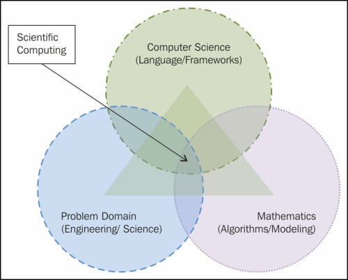
Scientific computing as an interdisciplinary field
Scientific computing requires knowledge of the subject of the underlying problem to be solved (generally, it will be a problem from a science or engineering domain), a mathematical modeling capability with a sound idea of various numerical analysis techniques, and finally its efficient and high-performance implementation using computing techniques. It also requires application of computers; various peripherals, including networking devices, storage units, processing units, and mathematical and numerical analysis software; programming languages; and any database along with a good knowledge of the problem domain. The use of computation and related technologies has enabled newer applications, and scientists can infer new knowledge from existing data and processes.
In terms of computer science, scientific computing can be considered a numerical simulation of a mathematical model and domain data/information. The objective behind a simulation depends on the domain of the application under simulation. The objective can be to understand the cause behind an event, reconstruct a specific situation, optimize the process, or predict the occurrence of an event. There are several situations where numerical simulation is the only choice, or the best choice. There are some phenomena or situations where performing experiments is almost impossible, for example, climate research, astrophysics, and weather forecasts. In some other situations, actual experiments are not preferable, for example, to check the stability or strength of some material or product. Some experiments are very costly in terms of time/economy, such as car crashes or life science experiments. In such scenarios, scientific computing helps users analyze and solve problems without spending much time or cost.
A simple flow diagram of computation for a scientific application is depicted in the next diagram. The first step is to design a mathematical model for the problem under consideration. After the formulation of the mathematical model, the next step is to develop its algorithm. This algorithm is then implemented using a suitable programming language and an appropriate implementation framework. Selecting the programming language is a crucial decision that depends on the performance and processing requirements of the application. Another close decision is to finalize the framework to be used for the implementation. After deciding on the language and framework, the algorithm is implemented and sample simulations are performed. The results obtained from simulations are then analyzed for performance and correctness. If the result or performance of the implementation is not as per expectations, its causes should be determined. Then we need to go back to either reformulate the mathematical model, or redesign the algorithm or its implementation and again select the language and the framework.
A mathematical model is expressed by a set of suitable equations that describe most problems to the right extent of details. The algorithm represents the solution process in individual steps, and these will be implemented using a suitable programming language or scripting.
After implementation, there is an important step to perform—the simulation run of the implemented code. This involves designing the experimentation infrastructure, preparing or arranging the data/situation for simulation, preparing the scenario to simulate, and much more.
After completing a simulation run, result collection and its presentation are desired for the next step to analyze the results so as to test the validity of the simulation. If the results are not as they are expected, then this may require going back to one of the previous steps of the process to correct and repeat them. This situation is represented in the following figure in the form of dashed lines going back to some previous steps. If everything goes ahead perfectly, then the analysis will be the last step of the workflow, which is represented by double lines in this diagram:
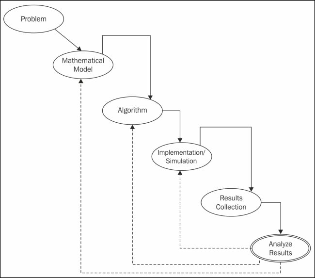
Various steps in a scientific computing workflow
The design and analysis of algorithms that solves any mathematical problem, specifically about science and engineering, is known as numerical analysis, and nowadays it is also called scientific computing. In scientific computing, the problems under consideration mainly deal with continuous values rather than discrete values. The latter are dealt with in other computer science problems. Generally saying, scientific computing solves problems that involve functions and equations with continuous variables, for example, time, distance, velocity, weight, height, size, temperature, density, pressure, stress, and much more.
Generally, problems of continuous mathematics have approximate solutions, as their exact solution is not always possible in a finite number of steps. Hence, these problems are solved using an iterative process that finally converges to an acceptable solution. The acceptable solution depends on the nature of the specific problem. Generally, the iterative process is not infinite, and after each iteration, the current solution gets closer to the desired solution for the purpose of simulation. Reviewing the accuracy of the solution and swift convergence to the solution form the gist of the scientific computing process.
There are well-established areas of science that use scientific computing to solve problems. They are as follows:
Computational fluid dynamics
Atmospheric science
Seismology
Structural analysis
Chemistry
Magnetohydrodynamics
Reservoir modeling
Global ocean/climate modeling
Astronomy/astrophysics
Cosmology
Environmental studies
Nuclear engineering
Recently, some emerging areas have also started harnessing the power of scientific computing. They include:
Biology
Economics
Materials research
Medical imaging
Animal science
Let's take a look at some problems that may be solved using scientific computing. The first problem is to study the behavior of a collision of two black holes, which is very difficult to understand theoretically and practically. Theoretically, this process is extremely complex, and it is almost impossible to perform it in a laboratory and study it live. But this phenomenon can be simulated in a computing laboratory with a proper and efficient implementation of a mathematical formulation of Einstein's general theory of relativity. However, this requires very high computational power, which can be achieved using advanced distributed computing infrastructure.
The second problem is related to engineering and designing. Consider a problem related to automobile testing called crash testing. To reduce the cost of performing a risky actual crash for testing, engineers and designers prefer to perform a computerized simulated crash test. Finally, consider the problem of designing a large house or factory. It is possible to construct a dummy model of the proposed infrastructure. But that requires a reasonable amount of time and is expensive. However, this designing can done using an architectural design tool, and this will save a lot of time and cost. There can be similar examples from bioinformatics and medical science, such as protein structure folding and modeling of infectious diseases. Studying protein structure folding is a very time-consuming process, but it can be efficiently completed using large-scale supercomputers or distributed computing systems. Similarly, modeling an infectious disease will save efforts and cost in the analysis of the effects of various parameters on a vaccination program for that disease.
These three examples are selected as they represent three different classes of problems that can be solved using scientific computing. The first problem is almost impossible. The second problem is possible, but it is risky up to a certain extent and it may result in severe damage. The final problem can be solved without any simulation and it is possible to duplicate it in real-life situations. However, it is costlier and more time-consuming than its simulation.
A simple strategy to find a solution for a complex computational problem is to first identify the difficult areas in the solution. Now, one by one, start replacing these small difficult parts with their solutions that will lead to the same solution or to a solution within the problem-specific permissible limit. In other words, the best idea is to reduce a large, complex problem to a set of smaller problems. Each of them may be complex or simple. Now each of the complex subproblems may be replaced with a similar and simple problem, and in this way, we ultimately get a simpler problem to solve. The basic idea is to combine the divide-and-conquer technique with the change of smaller complex problems with similar simple problems.
We should take care of two important points when adopting this idea. The first is that we need to search for a similar problem or a problem that has a solution from the same class. The second is that just after the replacement of one problem with another, we need to determine whether the ultimate solution is preserved within the tolerance limit, if not completely preserved. Some examples may be as follows:
Changing infinite-dimensional spaces in the problem to finite-dimensional spaces for simplicity
Change infinite processes with finite processes, such as replacing integrals or infinite series with finite summations or a derivative of finite differences
If feasible, then algebraic equations can be used to replace differential equations
Try replacing nonlinear problems with linear problems as linear problems are very simple to solve
If feasible, complicated functions can be changed to multiple simple functions to achieve simplicity
These scientific computational solutions generally produce approximate solutions. By approximate solution, we mean that instead of the exact desired solution, the obtained solution will be nearly similar to it. By nearly similar, we mean that it will be a sufficiently close solution to consider the practical or simulation successful, as they fulfill the purpose. This approximate, or similar, solution is caused by a number of sources. These sources can be divided into two categories: sources that arise before the computations begin, and those that occur during the computations.
The approximations that occur before the beginning of computations may be caused by one or more of the following:
Assumption or ignorance during modeling: There might be an assumption during the modeling process, and similarly ignorance or omission of the impact of a concept or phenomenon during modeling, that may result in the approximation or tolerable inaccuracy.
Data derived from observations or experiments: The inaccuracy may be in the data obtained from some devices that have low precision. During the computations, there are some constants, such as pi, whose values have to be approximated, and this is also an important cause of deviation from the correct result.
Prerequisite computations: The data may have been obtained from the results of previous experiments, or simulations may have had minor, acceptable inaccuracies that finally led to further approximations. Such prior processing may be a prerequisite of the subsequent experiments.
Approximation during computations occurs because of one or more of the following sources:
Simplification of the problem: As we have already suggested in this chapter, to solve large and complex problems, we should use a combination of "divide and conquer" and replacing a small, complex problem with a simpler one. This may result in approximations. Considering that we replaced an infinite series with a finite series will possibly cause approximations.
Truncation and rounding: A number of situations ask for rounding and truncation of the intermediate results. Similarly, the internal representation of floating-point numbers in computers and their arithmetic also leads to minor inaccuracies.
The approximate value of the final result of a computation problem may be the outcome of any combination of the various sources discussed previously. The accuracy of the final output may be reduced or increased depending on the problem being solved and the approach used to solve it.
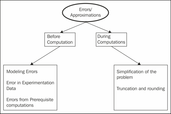
Taxonomy of errors and approximation in computations
Error analysis is a process used to observe the impact of such approximations on the accuracy of an algorithm or computational process. In the subsequent text, we are going to discuss the basic concepts associated with error analysis.
An observation may be made from the previous discussion on approximations that the errors can be considered as errors in the input data and they arose during the computations on this input data.
On a similar path, computation errors may again be divided into two categories: truncation errors and rounding errors. A truncation error is the result of reducing a complex problem to a simpler problem, for example, immature termination of iterations before the desired accuracy is achieved. A rounding error is the result of the precision used to represent numbers in the number system used for the computerized computation, and also the result of performing arithmetic on these numbers.
Ultimately, the amount of error that is significant or ignorable depends on the scale of the values. For example, an error of 10 in a final value of 15 is highly significant, while an error of 10 in a final value of 785 is not that significant. Moreover, the same error of 10 in obtaining the final value of 17,685 is ignorable. Generally, the impact of an error value is relative to the value of the result. If we know the magnitude of the final value to be obtained, then after looking at the value of the error, we can decide whether to ignore it or consider it as significant. If the error is significant, then we should start taking the corrective measures.
Let's discuss some important properties of problems and algorithms. Sensitivity or conditioning is a property of a problem. The problem under consideration can be called sensitive or insensitive, or it may be called well-conditioned or ill-conditioned. A problem is said to be insensitive or well-conditioned if, for a given relative change in input, the data will have a proportional relative final impact on the result. On the other hand, if the relative impact of the final result is considerably larger than the relative change in input data, then the problem will be considered a sensitive or ill-conditioned problem.
Assume that we have obtained the approximation y* by f mapping the data x, for example, y*=f(x). Now, if the actual result is y, then the small quantity y' =y*-y is called a forward error, and its estimation is called forward error analysis. Generally, it is very difficult to obtain this estimate. An alternative approach to this is to consider y* as the exact solution to the same problem with modified data, that is, y*=f(x'). Now, the quantity x*=x'-x is called a backward error in y*. Backward error analysis is the process of estimation of x*.
The answer to this question depends on the domain and application where you are going to apply the scientific computations. For example, if it is the calculation of the time to launch a missile, an error of 0.1 seconds will result in severe damage. On the other hand, if it is the calculation of the arrival time of a train, an error of 40 seconds will not lead to a big problem. Similarly, a small change in a medicine dosage can have a disastrous effect on the patient. Generally, if a computation error in an application is not related to loss of human lives or doesn't involve big costs, then it can be ignored. Otherwise, we need to take proper efforts to resolve the issue.
A type of approximation in scientific computing is introduced due to the representation of real numbers in computers. This approximation is further magnified by performing arithmetic operations on these real numbers. In this section, we will discuss this representation of real numbers, arithmetic operations on these numbers, and their possible impact on the results of the computation. These approximation errors not only arise in computerized computations, however; they may arise in non-computerized manual computation because of the rounding done to reduce the complexity. However, it is not the case that these approximations arise only in the case of computerized computations. They can also be observed in non-computerized, manual computations because of rounding done to reduce complexities in calculations.
Before advancing the discussion of the computerized representation of real numbers, let's first recall the well-known scientific notation used in mathematics. In scientific notation, to simplify the representation of a very large or very small number into a short form, we write nearly the same quantity multiplied by some powers of 10. Also, in scientific notation, numbers are represented in the form of "a multiplied by 10 to the power b" that is, a X 10b. For example, 0.000000987654 and 987,654 can represented as 9.87654 x 10^-7 and 9.87654 x 10^5 respectively. In this representation, the exponent is an integer quantity and the coefficient is a real number called mantissa.
The Institute of Electrical and Electronics Engineers (IEEE) has standardized the floating-point number representation in IEEE 754. Most modern machines use this standard as it addresses most of the problems found in various floating-point number representations. The latest version of this standard is published in 2008 and is known as IEEE 754-2008. The standard defines arithmetic formats, interchange formats, rounding rules, operations, and exception handling. It also includes recommendations for advanced exception handling, additional operations, and evaluation of expressions, and tells us how to achieve reproducible results.
Python is a general-purpose high-level programming language that supports most programming paradigms, including procedural, object-oriented, imperative, aspect-oriented, and functional programming. It also supports logical programming using an extension. It is an interpreted language that helps programmers compose a program in fewer lines than the code for the same concept in C++, Java, or other languages. Python supports dynamic typing and automatic memory management. It has a large and comprehensive standard library, and now it also has support for a number of custom libraries for many specific tasks. It is very easy to install packages using package managers such as pip, easy_install, homebrew (OS X), apt-get (Linux), and others.
Python is an open source language; its interpreters are available for most operating systems, including Windows, Linux, OS X, and others. There are a number of tools available to convert a Python program into an executable form for different operating systems, for example, Py2exe and PyInstaller. This executable form is standalone code that does not require a Python interpreter for execution.
Python's guiding principles by Guido van Rossum, who is also known as the Benevolent Dictator For Life (BDFL), have been converted into some aphorism by Tim Peters and are available at https://www.python.org/dev/peps/pep-0020/. Let's discuss these with some explanations, as follows:
Beautiful is better than ugly: The philosophy behind this is to write programs for human readers, with simple expression syntax and consistent syntax and behavior for all programs.
Explicit is better than implicit: Most concepts are kept explicit, just like the explicit Boolean type. We have used an explicit literal value—true or false—for Boolean variables instead of depending on zero or nonzero integers. Still, it does support the integer-based Boolean concept. Nonzero values are treated as Boolean. Similarly, its
forloop can operate data structures without managing the variable. The same loop can iterate through tuples and characters in a string.Simple is better than complex: Memory allocation and the garbage collector manage allocation or deallocation of memory to avoid complexity. Another simplicity is introduced in the simple print statement. This avoids the use of file descriptors for simple printing. Moreover, objects automatically get converted to a printable form in comma-separated values.
Complex is better than complicated: Scientific computing concepts are complex, but this doesn't mean that the program will be complicated. Python programs are not complicated, even for very complex application. The "Pythonic" way is inherently simple, and the SciPy and NumPy packages are very good examples of this.
Flat is better than nested: Python provides a wide variety of modules in its standard library. Namespaces in Python are kept in a flat structure, so there is no need to use very long names, such as
java.net.socketinstead of a simple socket in Python. Python's standard library follows the batteries included philosophy. This standard library provides tools suitable for many tasks. For example, modules for various network protocols are supported for the development of rich Internet applications. Similarly, modules for graphic user interface programming, database programming, regular expressions, high-precision arithmetic, unit testing, and much more are bundled in the standard library. Some of the modules in the library include networking (socket,select,SocketServer,BaseHTTPServer,asyncore,asynchat,xmlrpclib, andSimpleXMLRPCServer), Internet protocols (urllib,httplib,ftplib,smtpd,smtplib,poplib,imaplib, andjson), database (anydbm,pickle,shelve,sqlite3, andmongodb), and parallel processing (subprocess,threading,multiprocessing, andqueue).Sparse is better than dense: The Python standard library is kept shallow and the Python package index maintains an exhaustive list of third-party packages meant for supporting in-depth operations for a topic. We can use
pipto install custom Python packages.Readability counts: The block structure of your program should be created using white spaces, and Python uses minimal punctuation in its syntax. As semicolons introduce blocks, no semicolons are needed at the end of the line. Semicolons are allowed but they are not required in every line of code. Similarly, in most situations, parentheses are not required for expressions. Python introduces inline documentation used to generate API documentation. Python's documentation is available at runtime and online.
Special cases aren't special enough to break the rules: The philosophy behind this is that everything in Python is an object. All built-in types are implemented as objects. The data types that represent numbers have methods. Even functions are themselves objects with methods.
Although practicality beats purity: Python supports multiple programming styles to give users the choice to select the style that is most suitable for their problem. It supports OOP, procedural, functional, and many more types of programming.
Errors should never pass silently: It uses the concept of exception handling to avoid handling errors at low level APIs so that they may be handled at a higher level while writing the program that uses these APIs. It supports the concept of standard exceptions with specific meanings, and users are allowed to define exceptions for custom error handling. To support debugging of code, the concept of traceback is provided. In Python programs, by default, the error handling mechanism prints a complete traceback pointing to the error in
stderr. The traceback includes the source filename, line number, and source code, if it is available.Unless explicitly silenced: To take care of some situations, there are options to let an error pass by silently. For these situations, we can use the
trystatement withoutexcept. There is also an option to convert an exception into a string.In the face of ambiguity, refuse the temptation to guess: Automatic type conversion is performed only when it is not surprising. For example, an operation between an integer operand with a float operand results in a float value.
There should be one—and preferably only one—obvious way to do it: This is very obvious. It requires elimination of all redundancy. Hence, it is easier to learn and remember.
Although that way may not be obvious at first unless you're Dutch: The way that we discussed in the previous point is applicable to the standard library. Of course, there will be redundancy in third-party modules. For example, we have support for multiple GUI APIs, such as as GTK, wxPython, and KDE. Similarly for web programming, we have Django, AppEngine, and Pyramid.
Now is better than never: This statement is meant to motivate users to adopt Python as their favorite tool. There is a concept of ctypes meant to wrap existing C/C++ shared libraries for use in Python programs.
Although never is often better than *right* now: With this philosophy, the Python Enhancement Proposals (PEP) processed a temporary moratorium (suspension) on all changes to the syntax, semantics, and built-in components for a specified period to promote the alternative development catch-up.
If the implementation is hard to explain, it's a bad idea and If the implementation is easy to explain, it may be a good idea: In Python all the changes to the syntax, new library modules, and APIs will be processed through a highly rigorous process of review and approval.
To be frank, if we're talking about the Python language alone, then we need to think about some option. Fortunately, we have support for NumPy, SciPy, IPython, and matplotlib, and this makes Python the best choice. We are going to discuss these libraries in subsequent chapters. The following are the comprehensive features of Python and the associated library that make Python preferable to the other alternatives such as MATLAB, R, and other programming languages. Mostly, there is no single alternative that possesses all of these features.
Python code is generally compact and inherently more readable in comparison to its alternatives for scientific computing. As discussed in the Python guiding principles, this is the impact of the design philosophy of Python.
Overall, the design of the Python language is highly convenient for scientific computing because Python supports multiple programming styles, including procedural, object-oriented, functional, and logic programming. The user has a wide range of choices and they can select the most suitable one for their problem. This is not the case with most of the available alternatives.
Python and the associated tools are freely available for use, and they are published as open source tools. This brings an added advantage of availability of their internal source code. On the other hand, most competing tools are costly proprietary products and their internal algorithms and concepts are not published for users.
Python supports interoperability with most existing technologies. We can call or use functions, code, packages, and objects written in different languages, such as MATLAB, C, C++, R, Fortran, and others. There are a number of options available to support this interoperability, such as Ctypes, Cython, and SWIG.
Python supports most platforms. So, it is a portable programming language, and its program written for one platform will result in almost the same output on any other platform if Python toolkits are available for that platform. The design principles behind Python have made it a highly extensible language, and that's why we have a large number of high-class libraries available for a number of different tasks.
Python supports a modular system to organize programs in the form of functions and classes in a namespace. The namespace system is very simple in order to keep learning and remembering the concepts easy. This also supports enhanced code reusability and maintenance.
The Python language offers a wide set of choices in graphics packages and tool sets. These toolkits and packages support graphic design, user interface designing, data visualization, and various other activities.
Python supports an exhaustive range of data structures, which is the most important component in the design and implementation of a program to perform scientific computations. Support for a dictionary is the most highlightable feature of the data structure functionality of the Python language.
Python's unit testing framework, named PyUnit, supports complete unit testing functionality for integration with the mypython program. It supports various important unit testing concepts, including test fixture, test cases, test suites, and test runner.
Owing to the batteries-included philosophy of Python, it supports a wide range of standard packages in its bundled library. As it is an extensible language, a number of well-tested custom-specific purpose libraries are available for a wide range of users. Let's briefly discus a few libraries used for scientific computations.
NumPy/SciPy is a package that supports most mathematical and statistical operations required for any scientific computation. The SymPy library provides functionality for symbolic computations of basic symbolic arithmetic, algebra, calculus, discrete mathematics, quantum physics, and more. PyTables is a package used to efficiently process datasets that have a large amount of data in the form of a hierarchical database. IPython facilitates the interactive computing feature of Python. It is a command shell that supports interactive computing in multiple programming languages. matplotlib is a library that supports plotting functionality for Python/NumPy. It supports plotting of various types of graphs, such as line plot, histogram, scatter plot, and 3D plot. SQLAlchemy is an object-relational mapping library for Python programming. By using this library, we can use the database capability for scientific computations with great performance and ease. Finally, it is time to introduce a toolkit written on top of the packages we just discussed and a number of other open source libraries and toolkits. This toolkit is named SageMath. It is a piece of open source mathematical software.
After discussing a lot of upsides of Python over the alternatives, if we start searching for some downsides, we will notice something important: the integrated development environment (IDE) of Python is not the most powerful IDE compared to the alternatives. As Python toolkits are arranged in the form of discrete packages and toolkits, some of them have a command-line interface. So, in the comparison of this feature, Python is lagging behind some alternatives on specific platforms, for example, MATLAB on Windows. However, this doesn't mean that Python is not that convenient; it is equally comparable and supports ease of use.
In this chapter, we discussed the basic concepts of scientific computing and its definitions. Then we covered the flow of the scientific computing process. Next, we briefly discussed some examples from a few science and engineering domains. After the examples, we explained an effective strategy to solve complex problems. After that, we covered the concept of approximation, errors, and related terms.
We also discussed the background of the Python language and its guiding principles. Finally, we discussed why Python is the most suitable choice for scientific computing.
In the next chapter, we will discuss various mathematical/numerical analysis concepts involved in scientific computing. We will also cover various Python packages, toolkits, and APIs for scientific computing.