Machine Learning Quick Reference

A statistical model is the approximation of the truth that has been captured through data and mathematics or statistics, and acts as an enabler here. This approximation is used to predict an event. A statistical model is nothing but a mathematical equation. 

For example, let's say we reach out to a bank for a home loan. What does the bank ask us? The first thing they would ask us to do is furnish lots of documents such as salary slips, identity proof documents, documents regarding the house we are going to purchase, a utility bill, the number of current loans we have, the number of dependants we have, and so on. All of these documents are nothing but the data that the bank would use to assess and check our creditworthiness:

What this means is that your creditworthiness is a function of the salary, number of loans, number of dependants, and so on. We can arrive at this equation or relationship mathematically.

In the next section, we will see how models learn and how the model can keep getting better.

The basic premise behind the learning curve is that the more time you spend doing something, the better you tend to get. Eventually, the time to perform a task keeps on plummeting. This is known by different names, such as improvement curve, progress curve, and startup function.

For example, when you start learning to drive a manual car, you undergo a learning cycle. Initially, you are extra careful about operating the break, clutch, and gear. You have to keep reminding yourself when and how to operate these components.

But, as the days go by and you continue practicing, your brain gets accustomed and trained to the entire process. With each passing day, your driving will keep getting smoother and your brain will react to the situation without any realization. This is called subconscious intelligence. You reach this stage with lots of practice and transition from a conscious intelligence to a subconscious intelligence that has got a cycle.

Machine learning

Let me define machine learning and its components so that you don't get bamboozled by lots of jargon when it gets thrown at you.

In the words of Tom Mitchell, "A computer program is said to learn from experience E with respect to some class of tasks T and performance measure P, if its performance at tasks in T, as measured by P, improves with experience E."Also, another theory says that machine learning is the field that gives computers the ability to learn without being explicitly programmed.

For example, if a computer has been given cases such as, [(father, mother), (uncle, aunt), (brother, sisters)], based on this, it needs to find out (son, ?). That is, given son, what will be the associated item? To solve this problem, a computer program will go through the previous records and try to understand and learn the association and pattern out of these combinations as it hops from one record to another. This is called learning, and it takes place through algorithms. With more records, that is, more experience, the machine gets smarter and smarter.

Let's take a look at the different branches of machine learning, as indicated in the following diagram:

We will explain the preceding diagram as follows:

• Supervised learning: In this type of learning, both the input variables and output variables are known to us. Here, we are supposed to establish a relationship between the input variables and the output, and the learning will be based on that. There are two types of problems under it, as follows:
  • Regression problem: It has got a continuous output. For example, a housing price dataset wherein the price of the house needs to be predicted based on input variables such as area, region, city, number of rooms, and so on. The price to be predicted is a continuous variable.
  • Classification: It has got a discrete output. For example, the prediction that an employee would leave an organization or not, based on salary, gender, the number of members in their family, and so on.
• Unsupervised learning: In this type of scenario, there is no output variable. We are supposed to extract a pattern based on all the variables given. For example, the segmentation of customers based on age, gender, income, and so on.
• Reinforcement learning: This is an area of machine learning wherein suitable action is taken to maximize reward. For example, training a dog to catch a ball and give it—we reward the dog if they carry out this action; otherwise, we tell them off, leading to a punishment.

Wright's model

In Wright's model, the learning curve function is defined as follows:

The variables are as follows:

• Y: The cumulative average time per unit
• X: The cumulative number of units produced
• a: Time required to produce the first unit
• b: Slope of the function when plotted on graph paper (log of the learning rate/log of 2)

The following curve has got a vertical axis (y axis) representing the learning with respect to a particular work and a horizontal axis that corresponds to the time taken to learn. A learning curve with a steep beginning can be comprehended as a sign of rapid progress. The following diagram shows Wright's Learning Curve Model:

However, the question that arises is, How is it connected to machine learning? We will discuss this in detail now.

Let's discuss a scenario that happens to be a supervised learning problem by going over the following steps:

1. We take the data and partition it into a training set (on which we are making the system learn and come out as a model) and a validation set (on which we are testing how well the system has learned).
2. The next step would be to take one instance (observation) of the training set and make use of it to estimate a model. The model error on the training set will be 0.
3. Finally, we would find out the model error on the validation data.

Step 2 and Step 3 are repeated by taking a number of instances (training size) such as 10, 50, and 100 and studying the training error and validation error, as well as their relationship with a number of instances (training size). This curve—or the relationship—is called a learning curve in a machine learning scenario.

 

Let's work on a combined power plant dataset. The features comprised hourly average ambient variables, that is, temperature (T), ambient pressure (AP), relative humidity (RH), and exhaust vacuum (V), to predict the net hourly electrical energy output (PE) of the plant:

# importing all the libraries
import pandas as pd
from sklearn.linear_model import LinearRegression
from sklearn.model_selection import learning_curve
import matplotlib.pyplot as plt

#reading the data
data= pd.read_excel("Powerplant.xlsx")

#Investigating the data
print(data.info())
data.head()

From this, we are able to see the data structure of the variables in the data:

The output can be seen as follows:

The second output gives you a good feel for the data.

The dataset has five variables, where ambient temperature (AT) and PE (target variable).

 

 

Let's vary the training size of the data and study the impact of it on learning. A list is created for train_size with varying training sizes, as shown in the following code:

# As discussed here we are trying to vary the size of training set
train_size = [1, 100, 500, 2000, 5000]
features = ['AT', 'V', 'AP', 'RH']
target = 'PE'
# estimating the training score & validation score
train_sizes, train_scores, validation_scores = learning_curve(estimator = LinearRegression(), X = data[features],y = data[target], train_sizes = train_size, cv = 5,scoring ='neg_mean_squared_error')

Let's generate the learning_curve:

# Generating the Learning_Curve
train_scores_mean =-train_scores.mean(axis =1)
validation_scores_mean =-validation_scores.mean(axis =1)
import matplotlib.pyplot as plt 
plt.style.use('seaborn')
plt.plot(train_sizes, train_scores_mean, label ='Train_error')
plt.plot(train_sizes, validation_scores_mean, label ='Validation_error')
plt.ylabel('MSE', fontsize =16)
plt.xlabel('Training set size', fontsize =16)
plt.title('Learning_Curves', fontsize = 20, y =1)
plt.legend()

We get the following output:

From the preceding plot, we can see that when the training size is just 1, the training error is 0, but the validation error shoots beyond 400.

As we go on increasing the training set's size (from 1 to 100), the training error continues rising. However, the validation error starts to plummet as the model performs better on the validation set. After the training size hits the 500 mark, the validation error and training error begin to converge. So, what can be inferred out of this? The performance of the model won't change, irrespective of the size of the training post. However, if you try to add more features, it might make a difference, as shown in the following diagram:

The preceding diagram shows that the validation and training curve have converged, so adding training data will not help at all. However, in the following diagram, the curves haven't converged, so adding training data will be a good idea:

So far, we have learned about the learning curve and its significance. However, it only comes into the picture once we tried fitting a curve on the available data and features. But what does curve fitting mean? Let's try to understand this.

Curve fitting is nothing but establishing a relationship between a number of features and a target. It helps in finding out what kind of association the features have with respect to the target. 

Establishing a relationship (curve fitting) is nothing but coming up with a mathematical function that should be able to explain the behavioral pattern in such a way that it comes across as a best fit for the dataset.

There are multiple reasons behind why we do curve fitting:

There are two types of curve fitting:

The following diagram shows the polynomial but exact fit:

The following diagram shows the line but exact fit:

Let's look at some different scenarios and study them to understand these differences.

Here, we will fit a curve for two numbers:

# importing libraries
 import numpy as np
 import matplotlib.pyplot as plt
 from scipy.optimize import curve_fit

# writing a function of Line
 def func(x, a, b):
 return a + b * x 
 x_d = np.linspace(0, 5, 2) # generating 2 numbers between 0 & 5
 y = func(x_d,1.5, 0.7) 
 y_noise = 0.3 * np.random.normal(size=x_d.size)
 y_d = y + y_noise
 plt.plot(x_d, y_d, 'b-', label='data')

 popt, pcov = curve_fit(func, x_d, y_d) # fitting the curve
 plt.plot(x_d, func(x_d, *popt), 'r-', label='fit')

From this, we will get the following output:

Here, we have used two points to fit the line and we can very well see that it becomes an exact fit. When introducing three points, we will get the following:

 x_d = np.linspace(0, 5, 3) # generating 3 numbers between 0 & 5

Run the entire code and focus on the output:

Now, you can see the drift and effect of noise. It has started to take the shape of a curve. A line might not be a good fit here (however, it's too early to say). It's no longer an exact fit.

What if we try to introduce 100 points and study the effect of that? By now, we know how to introduce the number of points.

By doing this, we get the following output:

This is not an exact fit, but rather a best fit that tries to generalize the whole dataset.

Residual

Residuals are the difference between an observed or true value and a predicted (fitted) value. For example, in the following diagram, one of the residuals is (A-B), where A is the observed value and B is the fitted value:

The preceding scatter plot depicts that we are fitting a line that could represent the behavior of all the data points. However, one thing that's noticeable is that the line doesn't pass through all of the points. Most of the points are off the line.

Note

The sum and mean of residuals will always be 0. ∑e =0 and mean of e =0.

Whenever we try to analyze data and finally make a prediction, there are two approaches that we consider, both of which were discovered by Leo Breiman, a Berkeley professor, in his paper titled Statistical Modeling: Two Cultures in 2001.

Any analysis needs data. An analysis can be as follows:

A vector of X (Features) undergoes a nature box, which translates into a response. A nature box tries to establish a relationship between X and Y. Typically, there are goals pertaining to this analysis, as follows:

Breiman states that, when it comes to solving business problems, there are two distinct approaches:

This is one of the most important steps of building a model and it can lead to lots of debate regarding whether we really need all three sets (train, dev, and test), and if so, what should be the breakup of those datasets. Let's understand these concepts.

After we have sufficient data to start modelling, the first thing we need to do is partition the data into three segments, that is, Training Set, DevelopmentSet, and Test Set:

Let's examine the goal of having these three sets:

Let's say in one scenario that we are trying to fit polynomials of various degrees:

After fitting the model, we calculate the training error for all the fitted models:

We cannot assess how good the model is based on the training error. If we do that, it will lead us to a biased model that might not be able to perform well on unseen data. To counter that, we need to head into the development set.

Size of the training, development, and test set

Typically, machine learning practitioners choose the size of the three sets in the ratio of 60:20:20 or 70:15:15. However, there is no hard and fast rule that states that the development and test sets should be of equal size. The following diagram shows the different sizes of the training, development, and test sets:

Another example of the three different sets is as follows:

But what about the scenarios where we have big data to deal with? For example, if we have 10,000,000 records or observations, how would we partition the data? In such a scenario, ML practitioners take most of the data for the training set—as much as 98-99%—and the rest gets divided up for the development and test sets. This is done so that the practitioner can take different kinds of scenarios into account. So, even if we have 1% of data for development and the same for the test test, we will end up with 100,000 records each, and that is a good number.

Before we get into modelling and try to figure out what the trade-off is, let's understand what bias and variance are from the following diagram:

There are two types of errors that are developed in the bias-variance trade off, as follows:

As the complexity of the algorithm keeps on increasing, the training error goes down. However, the development error or validation error keeps going down until a certain point, and then rises, as shown in the following diagram:

The preceding diagram can be explained as follows:

We will explain the preceding diagram as follows:

We should always strive for the fourth scenario, which depicts the training error being low, as well as a low development set error. In the preceding table, this is where we have to find out a bias variance trade-off, which is depicted by a vertical line.

Now, the following question arises: how we can counter overfitting? Let's find out the answer to this by moving on to the next section.

We have now got a fair understanding of what overfitting means when it comes to machine learning modeling. Just to reiterate, when the model learns the noise that has crept into the data, it is trying to learn the patterns that take place due to random chance, and so overfitting occurs. Due to this phenomenon, the model's generalization runs into jeopardy and it performs poorly on unseen data. As a result of that, the accuracy of the model takes a nosedive.

Can we combat this kind of phenomenon? The answer is yes. Regularization comes to the rescue. Let's figure out what it can offer and how it works.

Regularization is a technique that enables the model to not become complex to avoid overfitting.

Let's take a look at the following regression equation:

The loss function for this is as follows:

The loss function would help in getting the coefficients adjusted and retrieving the optimal one. In the case of noise in the training data, the coefficients wouldn't generalize well and would run into overfitting. Regularization helps get rid of this by making these estimates or coefficients drop toward 0.

Now, we will cover two types of regularization. In later chapters, the other types will be covered.

Ridge regression (L2)

Due to ridge regression, we need to make some changes to the loss function. The original loss function gets added by a shrinkage component:

Now, this modified loss function needs to be minimized to adjust the estimates or coefficients. Here, the lambda is tuning the parameter that regularizes the loss function. That is, it decides how much it should penalize the flexibility of the model. The flexibility of the model is dependent on the coefficients. If the coefficients of the model go up, the flexibility also goes up, which isn't a good sign for our model. Likewise, as the coefficients go down, the flexibility is restricted and the model starts to perform better. The shrinkage of each estimated parameter makes the model better here, and this is what ridge regression does. When lambda keeps going higher and higher, that is, λ → ∞, the penalty component rises, and the estimates start shrinking. However, when λ → 0, the penalty component decreases and starts to become an ordinary least square (OLS) for estimating unknown parameters in a linear regression.

Least absolute shrinkage and selection operator 

The least absolute shrinkage and selection operator (LASSO) is also called L1. In this case, the preceding penalty parameter is replaced by |βj|:

By minimizing the preceding function, the coefficients are found and adjusted. In this scenario, as lambda becomes larger, λ → ∞, the penalty component rises, and so estimates start shrinking and become 0 (it doesn't happen in the case of ridge regression; rather, it would just be close to 0).

We have already spoken about overfitting. It is something to do with the stability of a model since the real test of a model occurs when it works on unseen and new data. One of the most important aspects of a model is that it shouldn't pick up on noise, apart from regular patterns.

Validation is nothing but an assurance of the model being a relationship between the response and predictors as the outcome of input features and not noise. A good indicator of the model is not through training data and error. That's why we need cross-validation.

Here, we will stick with k-fold cross-validation and understand how it can be used.

K-fold cross-validation

Let's walk through the steps of k-fold cross-validation:

1. The data is divided into k-subsets.
2. One set is kept for testing/development and the model is built on the rest of the data (k-1). That is, the rest of the data forms the training data.

3. Step 2 is repeated k-times. That is, once the preceding step has been performed, we move on to the second set and it forms a test set. The rest of the (k-1) data is then available for building the model:

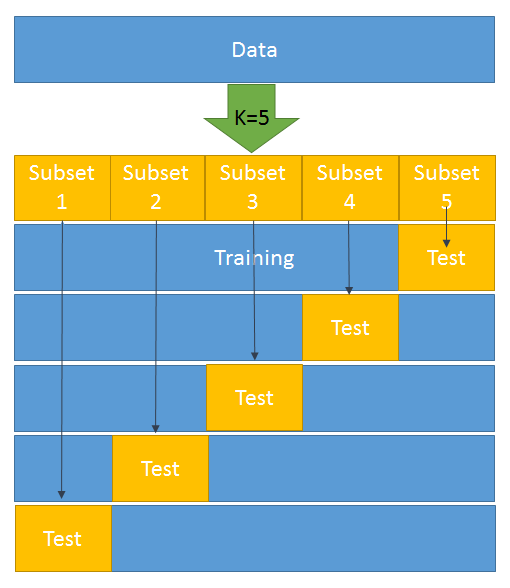
4. An error is calculated and an average is taken over all k-trials.

Every subset gets one chance to be a validation/test set since most of the data is used as a training set. This helps in reducing bias. At the same time, almost all the data is being used as validation set, which reduces variance.

As shown in the preceding diagram, k = 5 has been selected. This means that we have to divide the whole dataset into five subsets. In the first iteration, subset 5 becomes the test data and the rest becomes the training data. Likewise, in the second iteration, subset 4 turns into the test data and the rest becomes the training data. This goes on for five iterations.

Now, let's try to do this in Python by splitting the train and test data using the K neighbors classifier:

from sklearn.datasets import load_breast_cancer # importing the dataset
from sklearn.cross_validation import train_test_split,cross_val_score # it will help in splitting train & test
from sklearn.neighbors import KNeighborsClassifier
from sklearn import metrics

BC =load_breast_cancer() 
X = BC.data
y = BC.target

X_train, X_test, y_train, y_test = train_test_split(X, y, random_state=4)

knn = KNeighborsClassifier(n_neighbors=5)
knn.fit(X_train, y_train)
y_pred = knn.predict(X_test)
print(metrics.accuracy_score(y_test, y_pred))

knn = KNeighborsClassifier(n_neighbors=5)
scores = cross_val_score(knn, X, y, cv=10, scoring='accuracy')
print(scores)
print(scores.mean())

We can make use of cross-validation to find out which model is performing better by using the following code:

knn = KNeighborsClassifier(n_neighbors=20)
print(cross_val_score(knn, X, y, cv=10, scoring='accuracy').mean())

The 10-fold cross-validation is as follows:

# 10-fold cross-validation with logistic regression
from sklearn.linear_model import LogisticRegression
logreg = LogisticRegression()
print(cross_val_score(logreg, X, y, cv=10, scoring='accuracy').mean())

Before we get into the 0.632 rule of bootstrapping, we need to understand what bootstrapping is. Bootstrapping is the process wherein random sampling is performed with a replacement from a population that's comprised of n observations. In this scenario, a sample can have duplicate observations. For example, if the population is (2,3,4,5,6) and we are trying to draw two random samples of size 4 with replacement, then sample 1 will be (2,3,3,6) and sample 2 will be (4,4,6,2).

Now, let's delve into the 0.632 rule.

We have already seen that the estimate of the training error while using a prediction is 1/n ∑L(y_i,y-hat). This is nothing but the loss function:

Cross-validation is a way to estimate the expected output of a sample error:

However, in the case of k-fold cross-validation, it is as follows:

Here, the training data is X=(x1,x2.....,xn) and we take bootstrap samples from this set (z1,.....,zb) where each zi is a set of n samples. 

In this scenario, the following is our out-of-sample error:

Here, fb(xi) is the predicted value at xi from the model that's been fit to the bootstrap dataset.

Unfortunately, this is not a particularly good estimator because bootstrap samples that have been used to produce fb(xi) may have contained xi.OOSE solves the overfitting problem, but is still biased. This bias is due to non-distinct observations in the bootstrap samples that result from sampling with replacement. The average number of distinct observations in each sample is about 0.632n. To solve the bias problem, Efron and Tibshirani proposed the 0.632 estimator:

Let's look at some of the model evaluation techniques that are currently being used.

Confusion matrix

A confusion matrix is a table that helps in assessing how good the classification model is. It is used when true values/labels are known. Most beginners in the field of data science feel intimidated by the confusion matrix and think it looks more difficult to comprehend than it really is; let me tell you—it's pretty simple and easy.

Let's understand this by going through an example. Let's say that we have built a classification model that predicts whether a customer would like to buy a certain product or not. To do this, we need to assess the model on unseen data.

There are two classes:

• Yes: The customer will buy the product
• No: The customer will not buy the product

 From this, we have put the matrix together:

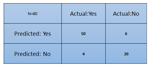
What are the inferences we can draw from the preceding matrix at first glance?

• The classifier has made a total of 80 predictions. What this means is that 80 customers were tested in total to find out whether he/she will buy the product or not.
• 54 customers bought the product and 26 didn't. 
• The classifier predicts that 56 customers will buy the product and that 24 won't:

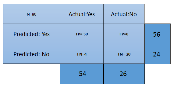
The different terms pertaining to the confusion matrix are as follows:

• True Positive (TP): These are the cases in which we predicted that the customer will buy the product and they did.
• True Negative (TN): These are the cases in which we predictedthat the customer won't buy the product and they didn't.
• False Positive (FP): We predicted Yes the customer will buy the product, but they didn't. This is known as a Type 1 error.
• False Negative (FN): We predicted No, but the customer bought the product. This is known as a Type 2 error.

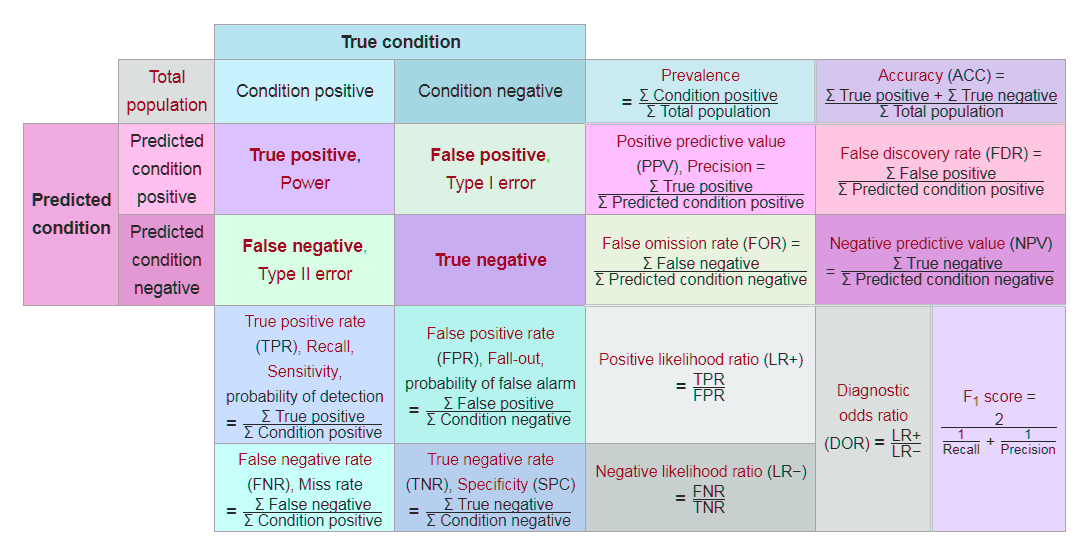
Now, let's talk about a few metrics that are required for the assessment of a classification model:

• Accuracy: This measures the overall accuracy of the classifier. To calculate this, we will use the following formula: (TP+TN)/Total cases. In the preceding scenario, the accuracy is (50+20)/80, which turns out to be 0.875. So, we can say that this classifier will predict correctly in 87.5% of scenarios.
• Misclassification rate: This measures how often the classifier has got the results wrong. The formula (FP+FN)/Total cases will give the result. In the preceding scenario, the misclassification rate is (6+4)/80, which is 0.125. So, in 12.5% of cases, it won't produce correct results. It can also be calculated as (1- Accuracy).
• TP rate: This is a measure of what the chances are that it would predict yes as the answer, and the answer actually is yes. The formula to calculate this is TP/(Actual:Yes). In this scenario, TPR = (50/54)= 0.92. It's also called Sensitivity or Recall.
• FP rate: This is a measure of what the chances are that it would predict yes, when the actual answer is no. The formula to calculate this rate is FP/(Actual:No). For the preceding example, FPR = (6/26)= 0.23.
• TN rate: This is a measure of what the chances are that it would predict no, when the answer is actually no. The formula to calculate this is TN/(Actual:No). In this scenario, TNR= (20/26)= 0.76. It can also be calculated using (1-FPR). It's also called Specificity. 
• Precision: This is a measure of correctness of the prediction of yes out of all the yes predictions. It finds out how many times a prediction of yes was made correctly out of total yes predictions. The formula to calculate this is TP/(Predicted:Yes). Here, Precision = (50/56)=0.89.
• Prevalence: This is a measure of how many yes were given out of the total sample. The formula is (Actual:Yes/ Total Sample). Here, this is 54/80 = 0.67.
• Null error rate: This is a measure of how wrong the classifier would be if it predicted just the majority class. The formula is (Actual:No/Total Sample). Here, this is 26/80=0.325.
• Cohen's Kappa value: This is a measure of how well the classifier performed compared to how well it would have performed simply by chance. 
• F-Score: This is a harmonic mean of recall and precision, that is, (2*Recall*Precision)/(Recall+Precision). It considers both Recall and Precision as important measures of a model's evaluation. The best value of the F-score is 1, wherein Recall and Precision are at their maximum. The worst value of the F-score is 0. The higher the score, the better the model is: 

We have come across many budding data scientists who would build a model and, in the name of evaluation, are just content with the overall accuracy. However, that's not the correct way to go about evaluating a model. For example, let's say there's a dataset that has got a response variable that has two categories: customers willing to buy the product and customers not willing to buy the product. Let's say that the dataset has 95% of customers not willing to buy the product and 5% of customers willing to buy it. Let's say that the classifier is able to correctly predict the majority class and not the minority class. So, if there are 100 observations, TP=0, TN= 95, and the rest misclassified, this will still result in 95% accuracy. However, it won't be right to conclude that this is a good model as it's not able to classify the minority class at all.

Hence, we need to look beyond accuracy so that we have a better judgement about the model. In this situation, Recall, Specificity, Precision, and the receiver operating characteristic (ROC) curve come to rescue. We learned about Recall, specificity, and precision in the previous section. Now, let's understand what the ROC curve is.

Most of the classifiers produce a score between 0 and 1. The next step occurs when we're setting up the threshold, and, based on this threshold, the classification is decided. Typically, 0.5 is the threshold—if it's more than 0.5, it creates a class, 1, and if the threshold is less than 0.5 it falls into another class, 2:

For ROC, every point between 0.0 and 1.0 is treated as a threshold, so the line of threshold keeps on moving from 0.0 to 1.0. The threshold will result in us having a TP, TN, FP, and FN. At every threshold, the following metrics are calculated:

The calculation of (TPR and FPR) starts from 0. When the threshold line is at 0, we will be able to classify all of the customers who are willing to buy (positive cases), whereas those who are not willing to buy will be misclassified as there will be too many false positives. This means that the threshold line will start moving toward the right from zero. As this happens, the false positive starts to decline and the true positive will continue increasing.

Finally, we will need to plot a graph of the TPR versus FPR after calculating them at every point of the threshold:

The red diagonal line represents the classification at random, that is, classification without the model. The perfect ROC curve will go along the y axis and will take the shape of an absolute triangle, which will pass through the top of the y axis. 

Binary classification has to apply techniques so that it can map independent variables to different labels. For example, a number of variables exist such as gender, income, number of existing loans, and payment on time/not, that get mapped to yield a score that helps us classify the customers into good customers (more propensity to pay) and bad customers.

Typically, everyone seems to be caught up with the misclassification rate or derived form since the area under curve (AUC) is known to be the best evaluator of our classification model. You get this rate by dividing the total number of misclassified examples by the total number of examples. But does this give us a fair assessment? Let's see. Here, we have a misclassification rate that keeps something important under wraps. More often than not, classifiers come up with a tuning parameter, the side effect of which tends to be favoring false positives over false negatives, or vice versa. Also, picking the AUC as sole model evaluator can act as a double whammy for us. AUC has got different misclassification costs for different classifiers, which is not desirable. This means that using this is equivalent to using different metrics to evaluate different classification rules.

As we have already discussed, the real test of any classifier takes place on the unseen data, and this takes a toll on the model by some decimal points. Adversely, if we have got scenarios like the preceding one, the decision support system will not be able to perform well. It will start producing misleading results.

H-measure overcomes the situation of incurring different misclassification costs for different classifiers. It needs a severity ratio as input, which examines how much more severe misclassifying a class 0 instance is than misclassifying a class 1 instance:

Severity Ratio = cost_0/cost_1

Here, cost_0 > 0 is the cost of misclassifying a class 0 datapoint as class 1.

It is sometimes more convenient to consider the normalized cost c = cost_0/(cost_0 + cost_1) instead. For example, severity.ratio = 2 implies that a false positive costs twice as much as a false negative.

Let's talk about a scenario wherein we have been given a dataset from a bank and it has got features pertaining to bank customers. These features comprise customer's income, age, gender, payment behavior, and so on. Once you take a look at the data dimension, you realize that there are 850 features. You are supposed to build a model to predict the customer who is going to default if a loan is given. Would you take all of these features and build the model?

The answer should be a clear no. The more features in a dataset, the more likely it is that the model will overfit. Although having fewer features doesn't guarantee that overfitting won't take place, it reduces the chance of that. Not a bad deal, right?

Dimensionality reduction is one of the ways to deal with this. It implies a reduction of dimensions in the feature space.

There are two ways this can be achieved:

Principal component analysis is a feature extraction technique that takes all of the variables into account and forms a linear combination of the variables. Later, the least important variable can be dropped while the most important part of that variable is retained.

Newly formed variables (components) are independent of each other, which can be a boon for a model-building process wherein data distribution is linearly separable. Linear models have the underlying assumption that variables are independent of each other.

To understand the functionality of PCA, we have to become familiar with a few terms:

Here, x is the mean.

In PCA, we find out the pattern of the data as follows: in the case of the dataset having high covariance when represented in n of dimensions, we represent those dimensions with a linear combination of the same n dimensions. These combinations are orthogonal to each other, which is the reason why they are independent of each other. Besides, dimension follows an order by variance. The top combination comes first.

Let's go over how PCA works by talking about the following steps:

Covariance Matrix = Z^TZ

In this chapter, we studied the statistical model, the learning curve, and curve fitting. We also studied two cultures that Leo Breiman introduced, which describe that any analysis needs data. We went through the different types of training, development, and test data, including their sizes. We studied regularization, which explains what overfitting means in machine learning modeling.

This chapter also explained cross validation and model selection, the 0.632 rule in bootstrapping, and also ROC and AUC in depth.

In the next chapter, we will study evaluating kernel learning, which is the most widely used approach in machine learning.